Extensions to the Su-Schrieffer-Heeger Model: Linear chains and their topological properties
Abstract
The Su-Schrieffer-Heeger (SSH) model describes the dynamics of spinless fermions in a one-dimensional lattice, with sublattices and , and governed by staggered hopping potentials and representing the intracell and intercell hopping energies, respectively. In this study, we extend the SSH model into three distinct types: a trimer chain, the generalized trimer chain, and a hexagonal chain. The trimer chain involves three sublattices with intracell and intercell hopping potentials and , respectively. The generalized trimer chain incorporates the intracell hopping and and intercell hopping and to differentiate the hopping energies between different sublattices in the chain. The hexagonal chain is composed of six sublattices with intracell hopping potential and intercell hopping potential . We utilize exact diagonalization to determine the bulk eigenvalues of the different models. We find that in the trimer and generalized trimer chain, the bulk eigenvalues exhibit conducting characteristics, independent of the hopping parameter, owing to the presence of a flat band situated along the Fermi energy. In the hexagonal chain, the bulk eigenvalues display semi-metallic characteristics in the region and metallic when . Furthermore, we investigate the presence of conducting edge states in the finite chains. The trimer and hexagonal chains show the presence of topologically protected edge states which are manifestations of one-dimensional topological insulators. We also established the bulk-boundary correspondence to calculate for the winding number that predicts the existence of localized edge states in the topological nontrivial phase.
I Introduction
Recently, topological insulators gained a lot of attention due to their unique electrical properties as opposed to regular insulators. Topological insulators (TI) are materials that have an energy band gap between the valence band and conducting band but have gapless edge states in one and two dimensions and surface states for 3D TI’s [1]. The different phases of matter can be classified according to Landau’s theory of symmetry breaking [2] which states that the different phases are due to their differences in symmetry. Furthermore, a phase transition occurs when there is a transition that changes the symmetry of the system [3]. However, the classification of phase transitions in topological insulators is beyond Landau’s theory. This means that TI’s can have different phases in zero temperature without breaking symmetry and the absence of classical phase transitions [3]. To differentiate these phases, we describe them by means of topological order [4]. These topological orders are generalized properties of zero temperature states having a finite band gap and does not change unless the system passes through a quantum phase transition, which is a singularity in the ground-state energy as a function of the parameters in the Hamiltonian [3], as the temperature is increased. Furthermore, TI’s also gained attention due to their possible applications in spintronics and quantum computing [5].

While most TI’s are studied in two and three dimensions, one-dimensional models give us a good arena to study because of their reduced complexity and accessibility to experiments [4]. A good toy model for understanding topological insulators is the Su-Schrieffer-Heeger (SSH) model [6]. The SSH model describes the hopping of spinless fermions in a one-dimensional (1D) lattice with staggered hopping potentials. It has a topological invariant winding number that shows the existence of edge states and differentiates the insulating phases through a quantum phase transition [1]. The SSH model was first applied in the study of the trans configuration of polyacetylene, which is the simplest conjugated polymer with alternating single and double covalent bonds [6]. Each of the carbon atoms in the chain form four covalent bonds. One is with the hydrogen atom and three are with the neighboring carbon atoms. The SSH model can be used to find out the properties of spinless fermions in a chain, such as trans-polyacetylene, with alternating double and single bonds, represented by and , as shown in Fig. 1.
Recent theoretical extensions of the SSH model include a 1D tripartite chain [7], 2D systems in square lattices [8] and arm-chair and zigzag graphene nanoribbons [9]. In this study, we extend the 1D SSH model into a tripartite chain and a hexagonal chain. We then determine the eigenstates and eigenvalues, i.e., the band structure of the extended models and establish the bulk-boundary correspondence to find out if topological edge states are present in the models. We introduce our models in Sec. II and investigate their corresponding eigenstates, energy spectra, and winding numbers in Sec. III.
II Theoretical Models
II.1 Trimer Chain
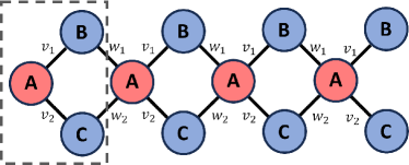
The trimer chain (see Fig. 2) is composed of three sublattices , , and arranged in a diamond chain with staggered hopping potentials and accounting for the intracell and intercell hopping energies, respectively.The single particle Hamiltonian for this trimer chain is given by
| (1) |
where is the cell index, and are the hopping potentials, and denotes hermitian conjugation. This gives the matrix elements , where the indices denote the cell number and denote the sublattice index. We also set the on-site potential to zero, i.e., . Furthermore, electron-electron interactions are neglected.

For the bulk, we set the boundary condition to be periodic, i.e., the Born-von Karman condition. We consider an effectively infinitely long chain because of the periodic boundary condition. This also implies that the bulk now is translationally invariant and Bloch’s theorem holds [1]. Our bulk Hamiltonian with the periodic boundary condition reads,
| (2) | ||||
To account for the periodicity, we introduce terms for the hopping between sites and , and , and vice versa.
II.2 Generalized trimer chain
The generalized trimer chain is a generalization of the trimer chain introduced in Sec. II.1. This model differentiates intracell and intercell hopping energies for , i.e., site to site in the same unit cell, and , i.e., site to site in the same unit cell, and , i.e., site to site in the neighboring unit cell, and , i.e., site to site in the neighboring unit cell, hopping energies (see Fig. 3). The single-particle Hamiltonian for this model is
| (3) | ||||
For the bulk part of the chain, we model it as a chain with periodic boundary conditions. The Hamiltonian for the bulk is
| (4) | ||||
The additional terms in the Hamiltonian account for the periodicity of the bulk.
Similar to the work of Bercioux et al. [7], we calculated the band structures of a tripartite lattice with infinite and finite unit cells. Lattice I of their work is similar to our trimer chain with intercell hopping in the , , and sublattices. Our generalized trimer chain generalizes the tripartite system which includes their Lattice II as a special case when and . To highlight the novelty of our work, we will show the eigenstates of the finite chains in the topological nontrivial and trivial regime. We will also calculate the winding number to establish the bulk-boundary correspondence of our three model chains.
II.3 Hexagonal chain

The hexagonal chain forms a resemblance to a 1D graphene armchair ribbon, as shown in Fig. 4. It consists of six sublattices and staggered hopping potentials and for the intracell and intercell hopping, respectively. The single-particle Hamiltonian for this hexagonal chain is
| (5) | ||||
where is the unit cell index. The elements of the Hamiltonian matrix are given by where and . The Hamiltonian for the bulk part of the chain modeled using periodic boundary conditions is
| (6) | ||||
III Eigenvalues, eigenstates, and the winding number
III.1 Trimer chain
Considering the bulk Hamiltonian of the trimer chain, Eq. (2), the energy eigenvalues of the system can be determined using exact diagonalization. The Schrödinger equation for the bulk Hamiltonian in matrix form is given by
| (16) |
This gives the energy eigenvalues
| (17) |
where is the wave number taking up values in the first Brillouin zone [1]. There are three eigenvalues in Eq. (17). The first eigenvalue (zero energy) has energy coinciding with the Fermi Energy, i.e., [1]. By varying the magnitude of the hopping parameters and , a dispersion relation shown in Fig. 5 can be obtained.

The dispersion relation consists of five different scenarios concerned with the different magnitudes of the hopping parameter. Fig. 5(a) describes the system with and . Examining the figure, it can be seen that there exists a flat band situated at the Fermi level . This is due to which has a constant value and is independent on the wavenumber . This characteristic can be seen in all the configurations indicating that all of the configuration of the system is a conductor [10]. Furthermore, two flat bands can also be observed at regions . The same observations can be seen in Fig. 5(e) with flat bands situated at for and . The case for , Fig. 5(b), and , Fig. 5(d), show sinusoidal variations of the energy with respect to the wave number. A defined gap between the uppermost and the lowest energy band can be seen. Lastly, for the case where , Fig. 5(c), the uppermost and the lowest energy band crossed in the region indicating an intersection, at a point, between the two bands.

To consider the characteristics of the boundaries of the chain, we examine a finite trimer chain. For the extreme cases where or the chain breaks down into trimers. For the trivial case , it can be observed that all of the sites belong to a corresponding trimer. However, for the topological case where , there are sites that do not belong to a corresponding trimer. Since fermions in these sites do not hop, then these edge sites host zero-energy states given by .
To calculate for the eigenvalues of the finite trimer chain, we diagonalize the Hamiltonian given by
| (25) |
with
| (32) |
where for unit cells, the Hamiltonian is a matrix. By varying the hopping amplitude of the finite trimer chain, the eigenvalue spectra can be obtained (see Fig. 6). As observed from Fig. 6(a), zero-energy states span throughout the graph independent of the values of . This corresponds to the zero-energy eigenvalue that we calculated earlier for the bulk (see Eq. (17)). Notice that these states with zero energy are degenerate. In Fig. 6(a), there are states having the same zero energy. Furthermore, in the region where , there exists two additional zero-energy states that reside at the edges of the chain. These results are consistent with those found by Bercioux et al. [7]. This region is defined as the topologically nontrivial phase as opposed to the region where , which we define as the topologically trivial phase. As we will see later in this section, these regions have different topological invariants that distinguishes their topological phase. Additionally, a topological phase transition can be observed in the region where the hopping potentials are equal. Fig. 6(b) and (c) show the probability density for the corresponding unit cells. Fig. 6(b) shows an arbitrary state where wherein the probability density extends throughout the whole chain. In contrast, Fig. 6(c) shows a state where . As seen in this plot, the probability density is localized on both the left and right edges of the chain. These states are defined as edge states, where the wave function is localized on both edges of the chain and exponentially decaying into the bulk. These edge states are typical characteristics of a one-dimensional topological insulator [1].
III.2 Generalized trimer chain
Following the same procedure as in the previous subsection, we solve for the energy eigenvalues of the generalized trimer chain using exact diagonalization. The Schrödinger equation, using the bulk Hamiltonian in matrix representation, is given by
| (42) |
This gives the energy eigenvalues
| (43) | ||||
Notice that when we set and , we will arrive at the same energy eigenvalues as those for the trimer chain in Eq. (17). Shown in Fig. 7 are the plots of the energy eigenvalues of the generalized trimer chain with respect to the wave number . As seen from the plots, different combinations of the hopping potentials lead to the same conducting characteristics due to the flat band situated along the Fermi level. This band is due to the that we obtained. Furthermore, as expected, the configurations where and resemble the dispersion relations of the trimer chain shown in Fig. 5(c). A visible gap between the uppermost and lowest energy band can be seen in Fig. 7(c) in the case where one hopping parameter is zero () while the rest are equal. It can be generalized that this band gap will remain open until we reach the limit where or or both (see Fig. 7(d) and (e)).

To determine the characteristics of the finite generalized trimer chain, we consider a lattice composed of unit cells. We find that when only one of the hopping potentials is nonzero and the rest are set to zero, the chain breaks down into dimers and the isolated sites would host zero-energy states. To calculate for the eigenvalues of the generalized trimer chain, we diagonalize the Hamiltonian given by
| (51) |
with
| (58) |
where for a unit cell of the generalized trimer chain, the Hamiltonian is a matrix. Fig. 8(a) shows the eigenvalue spectra of the finite generalized trimer chain by varying the three parameters simultaneously while maintaining . Also, the topological nontrivial phase in the region , which we found earlier in the trimer chain (see Fig. 6(a)), motivated us to explore the generalized case where . This case is shown in Fig. 8(b) where we vary the value of in the range while maintaining and . As noticed from Fig. 8(b), the states which form the edges in the trimer chain are now gapped in the region where and . This gap only closes in the trimer chain limit where .

Fig. 8(c) shows a representative probability density located at non-zero energy levels. Fig. 8(d) shows the probability density of one of the degenerate states in the generalized trimer chain. Lastly, we examined the eigenstates in the region where , of which a representative probability density is shown in Fig. 8(e). Although these states are non-zero energy gapped states, it displays a unique characteristic where the probability density is only localized in one of the edges. They are known as chiral edge states [11], which resemble only half of the full edge states of the original SSH model. As we will show later in this section, these chiral edge states do not share the same winding number as the gapless zero-energy edge states observed in the trimer chain.
To establish the bulk-boundary correspondence of the trimer and generalized trimer chains, we express their bulk momentum-space Hamiltonian in terms of the basis states. Consider the following traceless and hermitian matrices, which are four of the matrices known as Gell-Mann matrices representing the basis of the group SU(3) [12],
| (71) |
The bulk momentum-space Hamiltonian of the trimer chain can then be expressed as,
| (72) |
in which the new basis and are linear combinations of the Gell-Mann matrices,
| (73) | ||||
where the normalization coefficients ensure that the basis states follow the same trace orthonormality condition as that of the Gell-Mann matrices, [12]. On the other hand, for the generalized trimer chain, the bulk momentum-space Hamiltonian can be expressed as,
| (74) |
We can see that Eq. (74) reduces to Eq. (72) in the limit and . To reduce the parameters imposed by the 4-dimensional vector of the bulk momentum-space Hamiltonian of the generalized trimer chain, we set , i.e., effectively reducing the free parameters from four to three. The bulk momentum-space Hamiltonian of the generalized trimer chain now reads,
| (75) |
Note that the Hamiltonian in Eq. (75) satisfies chiral symmetry with the corresponding chiral operator
| (79) |
where and .
To calculate for the topological invariant winding number, we project the bulk momentum-space Hamiltonians into their corresponding basis states. As for the Hamiltonian of the trimer chain, Eq. (72), it has resemblance with that of the bulk momentum-space Hamiltonian of the original SSH dimer. As such, we expect its trajectory in the space to look like the trajectory of the SSH Hamiltonian in space. From these trajectories, we can calculate the winding number by counting the number of times the trajectory orbits around the origin, i.e., around . We determine the following winding number for the trimer chain,
| (83) |
The winding number is a useful tool in predicting the existence of gapless localized edge states (states where the wave function of the system is localized on both edges of the chain [1]). As shown in Eq. (83), for the case where , we found that , thus indicating a trivial topology of the system characterized by the absence of localized edge states. On the other hand, the case where indicates a non-trivial topology where indicating the presence of a pair of gapless localized edge states. Furthermore, the case where leads to an undetermined indicating that the trajectory of is in direct contact with the origin. This case entails a topological phase transition, which shows that the only way to change the winding number of the trimer chain from to , or vice versa, is by closing the gap between the highest and lowest band of the trimer chain.

Extending our analysis to the generalized case, we plot the trajectory of the bulk-momentum space Hamiltonian of the generalized trimer chain, Eq. (75) in -space, as shown in Fig. 9(a). Here we are interested to see if the winding number changes or remains the same for different variations in the upper, , and lower, , intracell hopping parameters. We are particularly interested in this case due to the non-trivial topological nature of the trimer chain in the regime, as we have shown earlier in this section. As such, we would like to generalize the conditions for the existence of gapless localized edge states in the regime in terms of their winding numbers. As observed from Fig. 9(a) we determined the following winding numbers,
| (87) |
where for all cases. From this result, we can see that only in the trimer chain limit, i.e., , is the winding number where we have shown a localized edge state in Fig. 6(c). It is also the region where the gap closes at between the pair of positive and negative energy band in Fig. 8(b). The other configurations, on the other hand, in Eq. (87), with and , demonstrate a chiral edge state emerging from a non-zero energy state, which is quite different from the usual gapless localized edge states where the probability densities are localized on both edges of the chain [11].
III.3 Hexagonal chain
Solving for the bulk energy eigenvalues of the hexagonal chain requires us to solve Schrödinger’s equation given by
| (106) |
The energy eigenvalues of the hexagonal chain with varying hopping parameters can be calculated by numerically diagonalizing the matrix in Eq. (106). We do this using the GNU Octave computational tool software. The eigenvalues are shown in Fig. 10.

We see that Fig. 10(a) to 10(c) show an insulating system due to the presence of a band gap. Furthermore, in Fig. 10(d) where , a conical band structure can be seen at . This band structure displays gapless and linear conducting bands which are typical for a semi-metal [13]. Additionally, when , see Fig. 10(e), the chain shows conducting characteristics due to the flat band situated along the Fermi energy, , independent of the wave number . The eigenvalue spectra can be determined by diagonalizing the Hamiltonian given by
| (114) |
with
| (127) |
where for a unit cells hexagonal chain, the Hamiltonian is a matrix.
Shown in Fig. 11(a) is the eigenvalue spectra obtained by plotting the energy eigenvalues with and slowly tuning in the range . Furthermore, Fig. 11(b) and 11(c) show a representative extended state and an edge state of the finite hexagonal chain. A pair of zero energy edge states (one is shown in Fig. 11(c)) show up when is varied. Additionally, we observe a topological phase transition around . The representative extended state seen in Fig. 11(b) shows an arbitrary non-zero energy state. In this figure, it can be seen that the probability density is extended across the chain indicating the conducting characteristics of a trivial topology. In contrast, the edge state shown in Fig. 11(c) indicates that the probability density is localized at the edges of the chain revealing the nontrivial topology of the system.

To establish the bulk-boundary correspondence of the hexagonal chain, we express the bulk momentum-space Hamiltonian in terms of its basis states:
| (128) |
where , , and are
| (147) |
These matrices satisfy the orthonormality condition . They are 3 of the 35 matrices representing the basis of the group SU(6). Furthermore, we define the chiral symmetric operator,
| (154) |
where and . This chiral operator ensures that the energies of the system form chiral symmetric pairs.
The trajectories of the bulk momentum-space Hamiltonian of the hexagonal chain in -space, Eq. (128) with varying hopping parameters are shown in Fig. 9(b). The trajectory of Eq. (128) forms a cylindrical plot with radius and height . Thus, increasing the value of and will increase the radius and height, respectively. The same as the procedure introduced in the previous section, we determine the winding number to be
| (158) |
where we keep the value of . As seen from the calculation of the winding number, we expect a pair of localized edge states in the region where the winding number . An example of this edge state is shown in Fig. 11(c).
IV Conclusion
In summary, we extended the Su-Schrieffer-Heeger model into three distinct types: the trimer chain, the generalized trimer chain, and the hexagonal chain. The trimer chain is a one-dimensional lattice with sites , , and and staggered hopping potentials and for the intracell and intercell hopping energies. The generalized trimer chain is a generalization of the trimer chain with the hopping parameters , , , and to distinguish the to from the to hopping. Lastly, the hexagonal chain which is composed of six sublattices and staggered hopping potentials and for the intracell and intercell hopping.
Exact diagonalization was used to calculate the energy eigenvalues of the bulk and the finite systems of the extended models. For the trimer chain, we find that the bulk characteristic of the chain exhibits conducting characteristics due to the flat band situated along the fermi energy independent of the values of and . Furthermore, when the hopping potentials are equal, it is seen that the uppermost and lowermost bands meet at . The trimer chain’s finite structure shows the presence of gapless zero-energy edge states as well as a topological phase transition, properties that resemble the characteristic of a one-dimensional topological insulator. The bulk-boundary correspondence for the trimer chain also predicts the existence of these localized edge states through the winding number where we determine in the topological () regime. The bulk characteristic of the generalized trimer chain, on the other hand, also shows conducting characteristic due to the flat band situated along the Fermi level. In the generalized case where and/or , a visible band gap can be seen between the uppermost and the lowest bands. This band gap only closes at the limit when and . The bulk-boundary correspondence of the generalized trimer chain reveals that the gapless topological edge states (localized on both edges) are only present in the trimer chain limit when . Gapped chiral edge states on the other hand, i.e., localized only on the left or right boundary, show up in the region where . Lastly, for the hexagonal chain, the dispersion relations show that the model is a semi-metal when due to the absence of a band gap and a metal when due to the presence of degenerate flat bands at the Fermi level. The existence of gapless localized edge states is also observed in the finite hexagonal chain at around where the system is in the topological phase defined by a winding number .
Acknowledgements.
The authors are grateful to Rafael Bautista for insightful discussions.References
- Asbòth et al. [2016] J. K. K. Asbòth, L. Oroszlàny, and A. P. Pàlyi, A Short Course on Topological Insulators: Band Structure and Edge States in One and Two Dimensions (Springer, New York, 2016).
- Hasan and Kane [2010] M. Z. Hasan and C. L. Kane, Colloquium: Topological insulators, Rev. Mod. Phys. 82, 3045 (2010).
- Wen [2004] X.-G. Wen, Quantum Field Theory of Many-Body Systems (Oxford University Press, Oxford, U. K., 2004).
- Guo [2016] H.-M. Guo, A brief review on one-dimensional topological insulators and superconductors, Sci. China-Phys. Mech. Astron. 59, 637401 (2016).
- Moore [2010] J. E. Moore, The birth of topological insulators, Nature 464, 194 (2010).
- Su et al. [1979] W. P. Su, J. R. Schrieffer, and A. J. Heeger, Solitons in polyacetylene, Phys. Rev. Lett. 42, 1698 (1979).
- Bercioux et al. [2017] D. Bercioux, O. Dutta, and E. Rico, Solitons in one-dimensional lattices with a flat band, Ann. Phys. (Berlin) 529, 1600262 (2017).
- Obana et al. [2019] D. Obana, F. Liu, and K. Wakabayashi, Topological edge states in the Su-Schrieffer-Heeger model, Phys. Rev. B 100, 075437 (2019).
- Fujita et al. [1997] M. Fujita, M. Igami, and K. Nakada, Lattice distortion in nanographite ribbons, J. Phys. Soc. Jpn. 66, 1864 (1997).
- Simon [2013] S. Simon, The Oxford Solid State Basics (Oxford University Press, Oxford, U. K., 2013).
- Martinez Alvarez and Coutinho-Filho [2019] V. M. Martinez Alvarez and M. D. Coutinho-Filho, Edge states in trimer lattices, Phys. Rev. A 99, 013833 (2019).
- Haber [2017] H. Haber, Properties of the Gell-Mann matrices. PHYS 251 group theory and modern physics lecture notes. University of California, Santa Cruz. (2017).
- Wan et al. [2011] X. Wan, A. M. Turner, A. Vishwanath, and S. Y. Savrasov, Topological semi-metal and Fermi-arc surface states in the electronic structure of pyrochlore iridates, Phys. Rev. B 83, 205101 (2011).