Extension of Noether’s theorem in -symmetric systems and its experimental demonstration in an optical setup
Abstract
Noether’s theorem is one of the fundamental laws in physics, relating the symmetry of a physical system to its constant of motion and conservation law. On the other hand, there exist a variety of non-Hermitian parity-time ()-symmetric systems, which exhibit novel quantum properties and have attracted increasing interest. In this work, we extend Noether’s theorem to a class of significant -symmetric systems for which the eigenvalues of the -symmetric Hamiltonian change from purely real numbers to purely imaginary numbers, and introduce a generalized expectation value of an operator based on biorthogonal quantum mechanics. We find that the generalized expectation value of a time-independent operator is a constant of motion when the operator presents a standard symmetry in the -symmetry unbroken regime, or a chiral symmetry in the -symmetry broken regime. In addition, we experimentally investigate the extended Noether’s theorem in -symmetric single-qubit and two-qubit systems using an optical setup. Our experiment demonstrates the existence of the constant of motion and reveals how this constant of motion can be used to judge whether the -symmetry of a system is broken. Furthermore, a novel phenomenon of masking quantum information is first observed in a -symmetric two-qubit system. This study not only contributes to full understanding of the relation between symmetry and conservation law in -symmetric physics, but also has potential applications in quantum information theory and quantum communication protocols.
pacs:
03.65.Ca, 03.65.Yz, 11.30.Rd, 42.50.XaI Introduction
The subject of finding the symmetries of dynamics is of fundamental interest and has broad applications in physics, e.g., high-energy scattering experiments, control issues in mesoscopic physics and quantum cosmology Symmetry1 ; chiralsymmetry1 ; chiralsymmetry2 ; chiralsymmetry3 ; chiralsymmetry4 ; topological2 . On the other hand, by means of symmetries, one can generally make non-trivial inferences from complex systems, such as many-body systems, dissipative systems and non-Hermitian systems. As an important theorem which is related to symmetries, Noether’s theorem Noether1 has important applications in quantum physics and quantum information science Noether2 ; Ehrenfest1 ; Ehrenfest2 ; Ehrenfest3 ; Noetheranalysis ; Noethercurrents . Noether’s theorem states that every symmetry of dynamics implies a conservation law, and it was originally applied in Lagrangian approach in classical mechanics to uncover conserved quantities from symmetries of the Lagrangian. In many cases, the existence of these conserved quantities is very important for understanding the physical states and the properties of the systems Noether2 ; Ehrenfest2 ; Noetheranalysis ; Noethercurrents . The theorem applies also in quantum mechanics, and the most prominent example of Noether’s theorem is Ehrenfest’s theorem in closed systems Ehrenfest1 ; Ehrenfest
| (1) |
For an operator without explicit time dependence, it then follows that its expectation value is a constant of motion if it commutes with the Hermitian Hamiltonian . However, Ehrenfest’s theorem is not applicable for open systems Ehrenfest3 ; Ehrenfest ; open1 ; r2 ; r5 . Furthermore, even in closed systems, Ehrenfest’s conservation law cannot capture all features of symmetry when mixed states are considered Ehrenfest2 .
A natural extension of Noether’s theorem in non-Hermitian systems is to replace the Hermitian Hamiltonian with a non-Hermitian Hamiltonian , which turns eq. (1) into conservationlaws2 ; interwining1 ; interwining2 ; SRM . Up to now, based on the important intertwining relation interwining1 ; interwining2 ; SRM , several methods have been proposed to obtain conserved quantities, including spectral decomposition methods SDM1 ; SDM2 , recursive construction of intertwining operators RCM , sum-rules method SRM , Stokes parametrization approach SPA , and so on. Recently, the authors in ref. Ehrenfest4 investigated a manifestation of Noether’s theorem in non-Hermitian systems, where an inner product was defined as without its complex conjugation. In their framework, a generalized symmetry, which they termed pseudochirality, emerges naturally as the counterpart of the symmetry defined by the commutation relation in quantum mechanics. Some existing works Ehrenfest1 ; Ehrenfest2 ; Ehrenfest3 ; Ehrenfest ; Ehrenfest4 ; Noetheranalysis ; Noethercurrents ; conservationlaws2 ; open1 ; interwining1 ; interwining2 ; SRM ; SDM1 ; SDM2 ; RCM ; SPA ; r2 ; r5 enrich the understanding of obtaining conserved quantity beyond the Hermitian framework, whereas a full understanding of the relation between symmetry and conservation law, and practical methods for extracting expectation values in non-Hermitian systems, remain elusive. Therefore, in order to properly deal with conservation problems using Noether’s theorem and explore its potential applications in non-Hermitian systems, there is an urgent need to extend Noether’s theorem to non-Hermitian systems.
Over the past decades, there is considerable interest in the study of the dynamic properties of parity-time ()-symmetric non-Hermitian systems Non-Hermitian1 ; Non-Hermitian2 ; Non-Hermitian3 ; Non-Hermitian4 ; Non-Hermitian5 ; Non-Hermitianadd ; r1 ; r6 . The unique properties of -symmetric systems and their applications have been investigated in various physical systems topological1 ; Non-Hermitian6 ; optomechanics1 ; optomechanics2 ; photonics1 ; photonics2 ; microwave1 ; microwave2 ; r3 ; r4 . Moreover, many remarkable and unexpected quantum phenomena have been observed in -symmetric systems, such as critical phenomena CriticalPhenomena1 ; CriticalPhenomena2 , chiral population transfer energytransfer1 ; energytransfer2 , information retrieval InformationRetrieva1 ; InformationRetrieva2 , coherence flow InformationRetrieva3 and topological invariants invariant1 ; invariant2 . A complete characterization of conservation laws in -symmetric systems has been intensely explored RCM ; SDM2 . For example, based on the intertwining relation interwining1 ; interwining2 ; SRM , reference RCM has presented a complete set of conserved observables for a class of -symmetric Hamiltonians in a single-photon linear optical circuit. Moreover, in the pseudo-Hermitian representation of quantum mechanics SDM1 , reference APT has further implemented a model circuit of a generic anti--symmetric system. A counterintuitive energy-difference conserving dynamics has been observed APT , which is in stark contrast to the standard Hermitian dynamics keeping the system’s total energy constant. However, based on biorthogonal quantum mechanics, the manifestation of Noether’s theorem and a complete observation of conserved quantities in -symmetric systems and their consequences are still lacking both theoretically and experimentally.
In this work, we extend Noether’s theorem to a class of significant -symmetric non-Hermitian systems and introduce a generalized expectation value of a time-independent operator based on biorthogonal quantum mechanics Biorthogonal1 ; Biorthogonal2 ; Biorthogonal3 ; Biorthogonal4 . For the -symmetric systems considered here, the eigenvalues of the -symmetric Hamiltonian change from purely real numbers to purely imaginary numbers. Such -symmetric systems have been widely used to investigate the dynamics of non-Hermitian systems in the presence of balanced gain and loss RCM ; Ehrenfest4 ; photonics1 ; CriticalPhenomena1 ; InformationRetrieva1 ; InformationRetrieva2 ; InformationRetrieva3 . Our work shows that the extended Noether’s theorem can be used to deal with conservation law problems about pure states and mixed states. Remarkably, we find that for an operator without explicit time dependence, its generalized expectation value is a constant of motion if presents a standard symmetry in the -symmetry unbroken regime, or a chiral symmetry in the -symmetry broken regime. In addition, we experimentally investigate the extended Noether’s theorem in -symmetric single-qubit and two-qubit systems using an optical setup. Several novel results are found. First, our experiment demonstrates the existence of the constant of motion. Second, our experiment reveals that the constant of motion can be used to judge whether the symmetry of a system is broken. Last, our experiment reveals the phenomenon of masking quantum information masking1 ; masking2 in a -symmetric two-qubit system.
II Extension of Noether’s theorem in -symmetric systems
To extend Noether’s theorem to -symmetric systems, the biorthogonal quantum mechanics Biorthogonal1 ; Biorthogonal2 ; Biorthogonal3 ; Biorthogonal4 is applied. In biorthogonal quantum mechanics, the inner product is defined as
| (2) |
where () is an arbitrary pure state with its associated state (), and and are left and right eigenstates of a non-Hermitian Hamiltonian (Appendixes A.1 and A.2).
Here, we use () to denote a density operator in standard (biorthogonal) quantum mechanics. Without loss of generality, let us consider the -symmetric system to be in a mixed state , is the probability of the system being in a pure state , with . With the inner product introduced in eq. (2), a generalized expectation value of an operator can be defined (see Appendix A.3)
| (3) | |||||
| (4) |
where is the generalized expectation value of the operator for an arbitrary pure state . Equation (3) provides a natural generalization of expectation value of an operator for an arbitrary quantum state, either a mixed state or a pure state.
As one of the main contributions of this work, we find that the temporal evolution of the expectation value of the operator follows two different forms (see Appendix A.3 for the detailed derivation)
| (5) | |||
| (6) |
where . Equation (5) corresponds to the case when the system works in the -symmetry unbroken regime, while eq. (6) corresponds to the case when the system works in the -symmetry broken regime. From eq. (5), one can see that the expectation value is a constant of motion if the Hamiltonian and the time-independent operator satisfy the commutation relation , i.e., the operator presents a standard symmetry in the -symmetry unbroken regime Symmetry1 . On the other hand, eq. (6) implies that the expectation value is also a constant of motion if and satisfy the anti-commutation relation , i.e., presents a chiral symmetry in the -symmetry broken regime chiralsymmetry1 .
To understand the above results intuitively, let us consider a -symmetric single-qubit system where the eigenvalues of the Hamiltonian change from real (in the -symmetry unbroken regime), to purely imaginary (in the -symmetry broken regime). The Hamiltonian for this system is given by (hereafter, we assume )
| (7) |
where is the non-Hermitian part of the Hamiltonian governing gain and loss Non-Hermitian1 ; non-Hermitianadd . The parameter is an energy scale, is a coefficient representing the degree of non-Hermiticity, and are the standard Pauli operators. The eigenvalues of are given by and , which are real numbers for (the -symmetry unbroken regime), while purely imaginary numbers for (the -symmetry broken regime). The right eigenvectors of are and , while the left eigenvectors of are and (Appendix A.2). Here, , , and satisfy to satisfy the biorthogonality and closure relations.
The Hamiltonian (7) can be considered as a deformed Pauli operator, , in view of the biorthogonal partners and (Appendixes A.1 and A.2). If a time-independent operator can be expressed in the form
| (8) |
where and are arbitrary nonzero coefficients, one can easily verify . Thus, according to eq. (5), the expectation value is a constant of motion in the -symmetry unbroken regime. On the other hand, if a time-independent operator can be expressed in the form
| (9) |
where is an arbitrary nonzero coefficient, one can obtain . In this case, according to eq. (6), the expectation value is a constant of motion in the -symmetry broken regime.
From an experimental point of view, in order to keep the expectation value as a real number, the chosen operator should be Hermitian in biorthogonal quantum mechanics (see Appendix A.4). Therefore, in the subsequent discussion, the coefficients and in eq. (8) are chosen as real numbers, and the coefficient in eq. (9) is chosen as a purely imaginary number.
III Experimental setup
III.1 Single-qubit case
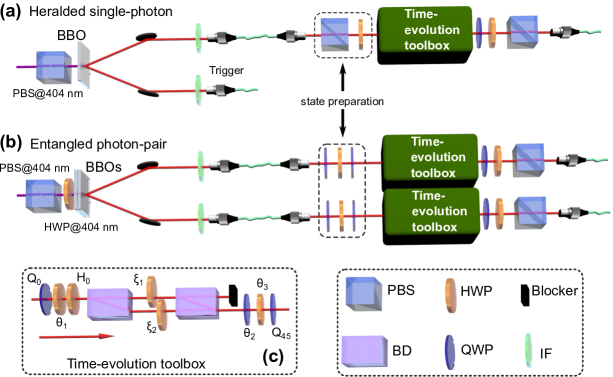
The apparatus for the initial state preparation in a single-photon system is illustrated in Figure 1a, where a single photon acts as the qubit. A photon pair is generated through a type-I phase-matched spontaneous parametric down-conversion process. The idler photon is detected by a single photon detector as a trigger. The qubit is encoded by the polarization of the heralded single photon, with and . The initial state is prepared by a polarization beam splitter (PBS) and a half-wave plate (HWP). Then the photon is injected into a time-evolution toolbox, which outputs the desired time-evolved state. In our experiment, the time-evolved state is accessed by enforcing the time-evolution operator =exp() at any given time on the initial state. Here, the Hamiltonian is the one given by eq. (7). As depicted in Figure 1c, the time-evolution toolbox implements the time-evolution operator by decomposing it into basic operations (see Appendix A.5)
| (10) | |||||
where the loss-dependent operator
| (11) |
is realized by a combination of two beam displacers (BDs) and two HWPs with setting angles and ( is fixed with in our experiment). Moreover, and are the rotation operators of the HWP and quarter-wave plate (QWP), respectively.
The time-evolved states in the -symmetric single-qubit system is given by InformationRetrieva1 ; rho1 ; rho2
| (12) |
where is the initial density matrix and is the experimental density matrix at any given time in standard quantum mechanics. The density matrix can be constructed via quantum state tomography Tomography ; Tomography1 . For the single-qubit system, we project the photon onto 4 bases . In addition, we note that the density matrix in biorthogonal quantum mechanics can be reversely extracted from the density matrix in standard quantum mechanics (Appendix A.6). On the other hand, the density matrix in biorthogonal quantum mechanics can be obtained according to the following relationships (Appendix A.7)
| (13) | |||
| (14) |
where =exp() and =exp() are time-evolution operators, and is the initial density matrix in biorthogonal quantum mechanics. Equations (13) and (14) correspond to the cases when the system evolves in the -symmetry unbroken regime and -symmetry broken regime, respectively.
III.2 Two-qubit case
The apparatus for the initial state preparation in a two-photon system is illustrated in Figure 1b. The entangled states in the experiment are generated through a type-II phase-matched spontaneous parametric down-conversion. Then two combinations of HWPs and QWPs (i.e., the upper and lower parts in the dashed box) operating on each photon, eliminate the influence caused by the fibres, therefore preparing the initial state. Then each photon is injected into a -symmetric time evolution toolbox. The dynamical evolution of quantum states in this case is similarly given by equation (12), where the time-evolution nonunitary operator is now given by . Here, () is the time-evolution nonunitary operator of qubit in the two-qubit system. Experimentally, we reconstruct the density matrix at any given time via quantum state tomography after each of the two photons passes through the time-evolution toolbox. Essentially, we project the two-qubit state onto 16 basis states through a combination of QWP, HWP and PBS, and then perform a maximum-likelihood estimation of the density matrix Tomography ; Tomography1 .
III.3 Device parameters
For the single-qubit case, the photon pair is generated through a type-I phase-matched spontaneous parametric down-conversion process by pumping a nonlinear -barium-borate (BBO) crystal with a 404 nm pump laser, where the BBO crystal is 3 mm thick. The power of the pump laser is 130 mW. The bandwidth of the interference filter (IF) is 10 nm. This yields a maximum count of 60,000 per second. The quantum state is measured by performing standard state tomography, i.e., projecting the state onto 4 bases , and the corresponding angles of QWP-HWP are , , , , and , respectively.
For the two-qubit case, the entangled states in the experiment are generated through a type-II phase-matched spontaneous parametric down-conversion, by pumping two BBO crystals with a 404 nm pump laser, where each BBO crystal is 0.4 mm thick and the optical axes are perpendicular to each other. The measurement of the photon source yields a maximum of 10,000 photon counts over 1.5 s after the 10 nm IF. Here, the quantum state is measured by performing standard state tomography, i.e., projecting the state onto 16 bases {, , , , , , , , , , , , , , , }, where , , and .
IV Experimental and theoretical results
IV.1 Expectation values of operators in a -symmetric single-qubit system
As two results derived from Noether’s theorem, equations (8) and (9) tell us that the expectation value is a constant of motion if
| (15) |
and
| (16) |
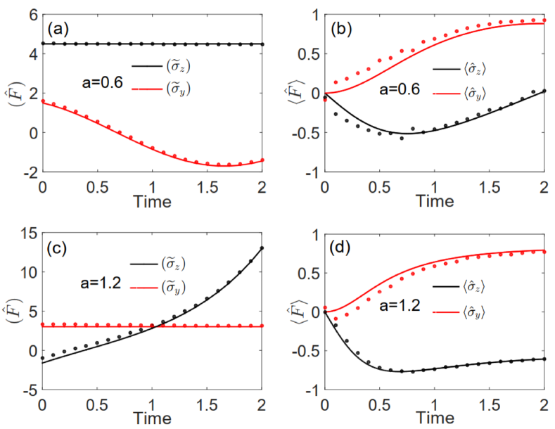
for the -symmetry unbroken and broken cases, respectively. We experimentally confirm this prediction in a -symmetric single-qubit system. As shown in Figure 2a, in the -symmetry unbroken regime, is a constant of motion, whereas changes over time. Interestingly, in contrast to Figure 2a, Figure 2c shows that in the -symmetry broken regime, is a constant of motion, while changes over time. The experimental results here agree well with the theoretical simulation results. As a contrast, we also measure the expectation values of and in standard quantum mechanics, shown in Figures 2b and 2d. One can see from Figures 2b and 2d that both and change over time in the -symmetry unbroken or broken regime, i.e., one cannot obtain a constant of motion. Hence, according to the temporal evolution of expectation values of and , one can judge whether the system works in the -symmetry unbroken or broken regime.
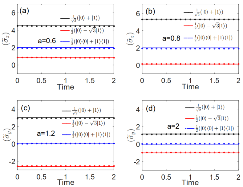
On the other hand, since our experimental apparatus is quite general and capable of implementing a broad class of nonunitary operators, we are able to investigate the role of non-Hermiticities and the effects of initial states on the temporal evolution of expectation values. It can be clearly seen from Figures 3a and 3b that with different initial states, is always a constant in the -symmetry unbroken regime even though the initial state is a mixed state. However, the expectation value is dependent on the initial states. Comparing Figure 3a with Figure 3b, one can see that the expectation value gradually increases when the parameter (representing the degree of non-Hermiticity) increases. Similarly, Figures 3c and 3d show that in -symmetry broken regime, is always a constant for different initial states even though the initial state is a mixed state, and the expectation value gradually decreases when the parameter increases.
IV.2 Expectation values of operators in a -symmetric two-qubit system
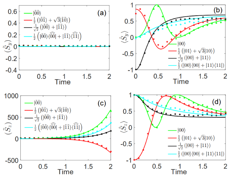
We further study the evolution of a two-qubit system using the optical setup shown in Figure 1b. The Hamiltonian of the two-qubit system is described by =+=+, with =+, =+, and =+. Here, and are the standard Pauli operators for the photonic qubit . The parameter is still the energy scale. For different initial states, the temporal evolutions of expectation values in the two-qubit system are plotted in Figure 4. The observable operators in Figure 4a and Figure 4c are chosen as =+ and =+, respectively. Here, and are deformed Pauli operators for the qubit in biorthogonal quantum mechanics. One can verify and . As expected, Figures 4a and 4c show that remains unchanged, whereas changes quickly in the -symmetry broken regime (). Remarkably, it’s worth noting that the expectation value is zero, which is independent of the initial states. Taking an information-theoretic perspective on this phenomenon, one can thus conclude that the information of the initial states is masked when measuring the expectation value , while the information of the initial states can be disclosed by measuring the expectation value . In addition, Figures 4b and 4d show that both and depend on the initial states and change over time, i.e., the phenomenon of masking quantum information does not exist in standard quantum mechanics. Hence, the masking of quantum information is a unique phenomenon in biorthogonal quantum mechanics.
V CONCLUSION
We have extended Noether’s theorem to a class of significant -symmetric non-Hermitian systems and introduced a generalized expectation value of a time-independent operator based on biorthogonal quantum mechanics. We have demonstrated that in the -symmetry unbroken regime, the generalized expectation value of a time-independent operator is a constant of motion, if the time-independent operator and the non-Hermitian Hamiltonian satisfy the commutation relation, i.e., the operator presents a standard symmetry. Moreover, even in the -symmetry broken regime, the expectation value of a time-independent operator is still a constant of motion provided the operator and the non-Hermitian Hamiltonian satisfy the anti-commutation relation, i.e., the operator presents a chiral symmetry. Furthermore, we have experimentally confirmed our predictions in -symmetric single-qubit and two-qubit systems by using an optical setup. Our experiment has demonstrated the existence of the predicted constant of motion. Meanwhile, a novel phenomenon of masking quantum information is first observed in a -symmetric two-qubit system. The extended Noether’s theorem not only contributes to a full understanding of the relation between symmetry and conservation law in -symmetric physics, but also has potential applications in quantum information theory and quantum communication protocols.
The present work has some elements in common with previous works on obtaining conserved quantity in non-Hermitian systems, especially the idea of using pseudo-Hermiticity (equivalently, the intertwining relation) interwining1 ; interwining2 ; SRM ; SDM1 ; SDM2 . Therefore, we here address the difference between our work and previous works. As shown in Refs. interwining1 ; interwining2 , every Hamiltonian with a real spectrum is pseudo-Hermitian, and all the -symmetric non-Hermitian Hamiltonians belong to the so-called pseudo-Hermitian Hamiltonians. In the pseudo-Hermitian representation of quantum mechanics, the expectation value of a time-independent operator is a conserved quantity provided the intertwining relation, , is satisfied. In principle, a complete set of conserved observables can be obtained by numerically solving a set of -dimensional linear intertwining relation SRM ; SDM1 ; SDM2 ; RCM ; SPA . However, a common problem, which one may encounter via pseudo-Hermiticity (intertwining relation), is how to connect the conserved quantities with the symmetries of dynamics. Compared with previous works interwining1 ; interwining2 ; SRM ; SDM1 ; SDM2 ; RCM ; SPA , the main difference of our work is that by introducing a generalized expectation value of an operator based on biorthogonal quantum mechanics, we connect two important symmetries with conserved operators in the -symmetry unbroken and broken regimes, respectively. We remark that the proposed standard symmetry and the chiral symmetry are essentially different from the intertwining relation , because of and in -symmetric systems.
We note that the extended Noether’s theorem is always valid for such -symmetric systems provided the eigenvalues of change from purely real numbers to purely imaginary numbers; or equivalently, exhibits an exceptional point of the order of the system’s dimension. As an example, consider a 3-dimensional -symmetric system SDM2 , for which the Hamiltonian reads , where and are the 3-dimensional angular momentum operators. Such a -symmetric Hamiltonian has a third-order exceptional point at and its spectrum also changes from real to purely imaginary SDM2 . Then, based on the extended Noether’s theorem, one can quickly find its conserved quantities in the -symmetry unbroken and broken regimes, respectively.
For any quantum system, whose Hamiltonian can be simplified to the form in eq. (7), the extended Noether’s theorem presented in this work can be implemented straightforwardly. Note that for the simplified Hamiltonian, arbitrary dressed states can be chosen as basis states as long as the dressed states satisfy the biorthogonality and closure relations. This might lead to a useful step toward realizing fast symmetry discrimination and conserved quantity acquisition for multi-qubit -symmetric systems. Moreover, in above discussion, we focus on the case of an operator without explicit time dependence. However, the derived equations (5,6) also work well in a general case i.e., the operator is time-dependent. Then, one may obtain constant of motion for a time-dependent operator in a time-dependent -symmetric system, which may be interesting and attractive. Furthermore, in some sense, the -symmetric Hamiltonian in eq. (7) has parallels with non-Hermitian topological phases topological1 ; topological2 and the extended classification of topological classes chiralsymmetry3 ; chiralsymmetry4 . The discovery of the relation between conserved quantities and non-Hermitian topological invariants invariant1 ; invariant2 is also interesting and attractive, which is a fascinating field where further extension of this work may be explored.
ACKNOWLEDGEMENT
This work was supported by the National Natural Science Foundation of China (NSFC) (Grants Nos. 12264040, 12204311, 11804228, 11865013 and U21A20436), Jiangxi Natural Science Foundation (20212BAB211018, 20192ACBL20051), the project of Jiangxi Province Higher educational Science and Technology Program (Grant Nos. GJJ190891, GJJ211735), and Key-Area Research and Development Program of Guang Dong province (2018B03-0326001). F.N. is supported in part by Nippon Telegraph and Telephone Corporation (NTT) Research, the Japan Science and Technology Agency (JST) [via the Quantum Leap Flagship Program (Q-LEAP), and the Moonshot RD Grant Number JPMJMS2061], the Japan Society for the Promotion of Science (JSPS) [via the Grants-in-Aid for Scientific Research (KAKENHI) Grant No. JP20H00134], the Army Research Office (ARO) (Grant No. W911NF-18-1-0358), the Asian Office of Aerospace Research and Development (AOARD) (via Grant No. FA2386-20-1-4069), and the Foundational Questions Institute Fund (FQXi) via Grant No. FQXi-IAF19-06.
References
- (1) A. Altland and M. R. Zirnbauer, “Nonstandard Symmetry Classes in Mesoscopic Normal-Superconducting Hybrid Structures,” Phys. Rev. B 55, 1142-1161 (1997).
- (2) S. Malzard, C. Poli, and H. Schomerus, “Topologically Protected Defect States in Open Photonic Systems with Non-Hermitian Charge-Conjugation and Parity-Time Symmetry,” Phys. Rev. Lett. 115, 200402 (2015).
- (3) Z. P. Gong, Y. Ashida, K. Kawabata, K. Takasan, S. Higashikawa, and M. Ueda, “Topological Phases of Non-Hermitian Systems,” Phys. Rev. X 8, 031079 (2018).
- (4) K. Kawabata, K. Shiozaki, M. Ueda, and M. Sato, “Symmetry and Topology in Non-Hermitian Physics,” Phys. Rev. X 9, 041015 (2019).
- (5) K. Y. Bliokh, J. Dressel, F. Nori, “Conservation of the spin and orbital angular momenta in electromagnetism,” New J. Phys. 16, 093037 (2014).
- (6) M. Li, X. Ni, M. Weiner, A. Alù, and A. B. Khanikaev, “Topological phases and nonreciprocal edge states in non-Hermitian Floquet insulators,” Phys. Rev. B 100, 045423 (2019).
- (7) A. E. Noether, “Invariante variations probleme,” Kgl Ges Wiss Nachr Göttingen,” Math. Phys. KI2, 235-257 (1918).
- (8) N. Ma, Y. Z. You and Z. Y. Meng, “Role of Noether’s Theorem at the Deconfined Quantum Critical Point,” Phys. Rev. Lett. 122, 175701 (2019).
- (9) R. Shankar, “Principles of Quantum Mechanics,” 2nd ed. (Springer, New York, 1994), https://doi.org/10.1007/978-1- 4757-0576-8.
- (10) I. Marvian, R. W. Spekkens, “Extending Noether’s theorem by quantifying the asymmetry of quantum states,” Nat. Commun. 5, 3821 (2014).
- (11) P. M. Zhang, M. Elbistan, P. A. Horvathy, P. Kosiński, “A generalized Noether theorem for scaling symmetry,” Eur. Phys. J. Plus 135, 223 (2020).
- (12) K. Y. Bliokh, A. Y. Bekshaev, F. Nori, “Dual electromagnetism: helicity, spin, momentum, and angular momentum,” New J. Phys. 15, 033026 (2013).
- (13) L. Burns, K. Y. Bliokh, F. Nori, J. Dressel, “Acoustic versus electromagnetic field theory: scalar, vector, spinor representations and the emergence of acoustic spin,” New J. Phys. 22, 053050 (2020).
- (14) J. J. García-Ripoll, V. M. Pérez-García, and V. Vekslerchik, “Construction of exact solutions by spatial translations in inhomogeneous nonlinear Schrödinger equations,” Phys. Rev. E 64, 056602 (2001).
- (15) Q. C. Wu, Y. H. Zhou, B. L. Ye, T. Liu and C. P. Yang, “Nonadiabatic quantum state engineering by time-dependent decoherence-free subspaces in open quantum systems,” New J. Phys. 23, 113005 (2021).
- (16) D. L. Li and C. Zheng, “Non-Hermitian Generalization of Rényi Entropy,” Entropy, 24, 1563 (2022).
- (17) X. E. Gao, D. L. Li, Z. H. Liu, and C. Zheng, “Recent progress in quantum simulation of non-Hermitian,” Acta Physica Sinica, 71, 240303 (2022).
- (18) H. Ramezani, T. Kottos, R. El-Ganainy, and D. N. Christodoulides, “Unidirectional nonlinear PT-symmetric optical structures,” Phys. Rev. A 82, 043803 (2010).
- (19) A. Mostafazadeh, “Pseudo-Hermiticity versus symmetry: The necessary condition for the reality of the spectrum of a non-Hermitian hamiltonian,” J. Math. Phys. 43, 205-214 (2002).
- (20) A. Mostafazadeh, “Exact -symmetry is equivalent to Hermiticity,” J. Phys. A: Math. Gen. 36, 7081-7091 (2003).
- (21) M. V. Berry, “Optical lattices with symmetry are not transparent,” J. Phys. A: Math. Theor. 41, 244007 (2008).
- (22) A. Mostafazadeh, “Pseudo-Hermitian representation of quantum mechanics,” Int. J. Geom. Methods Mod. Phys. 07, 1191-1306 (2010).
- (23) F. Ruzicka, K. S. Agarwal, Y. N. Joglekar, “Conserved quantities, exceptional points, and antilinear symmetries in non-Hermitian systems,” J. Phys.: Conf. Ser. 2038, 012021 (2021).
- (24) Z. Bian, L. Xiao, K. Wang, X. Zhan, F. A. Onanga, F. Ruzicka, W. Yi, Y. N. Joglekar, and P. Xue, “Conserved quantities in parity-time symmetric systems,” Phys. Rev. Research 2, 022039 (2020).
- (25) M. H. Teimourpour, R. El-Ganainy, A. Eisfeld, A. Szameit, and D. N. Christodoulides, “Light transport in -invariant photonic structures with hidden symmetries,” Phys. Rev. A 90, 053817 (2014).
- (26) J. D. H. Rivero and L. Ge, “Pseudochirality: A Manifestation of Noether’s Theorem in Non-Hermitian Systems,” Phys. Rev. Lett. 125, 083902 (2020).
- (27) C. M. Bender and S. Boettcher, “Real Spectra in Non-Hermitian Hamiltonians Having Symmetry,” Phys. Rev. Lett. 80, 5243-5246 (1998).
- (28) L. Ge, Y. D. Chong, and A. D. Stone, “Conservation relations and anisotropic transmission resonances in one-dimensional -symmetric photonic heterostructures,” Phys. Rev. A 85, 023802 (2012).
- (29) B. Peng, S. K. Ozdemir, F. C. Lei, F. Monifi, M. Gianfreda, G. L. Long, S. H. Fan, F. Nori, C. M. Bender and L. Yang, “Parity-time-symmetric whispering-gallery microcavities,” Nat. Phys. 10, 394-398 (2014).
- (30) H. Jing, S.K. Ozdemir, X. Y. Lu, J. Zhang, L. Yang, and F. Nori, “-Symmetric Phonon Laser,” Phys. Rev. Lett. 113, 053604 (2014).
- (31) V. V. Konotop, J. Yang, and D. A. Zezyulin, “Nonlinear waves in -symmetric systems,” Rev. Mod. Phys. 88, 035002 (2016).
- (32) R. E. Ganainy, K. G. Makris, M. Khajavikhan, Z. H. Musslimani, and D. N. Christodoulides, “Non-Hermitian physics and symmetry,” Nat. Phys. 14, 11-19 (2018).
- (33) O. Sigwarth and M. Christian, “Time reversal and reciprocity,” AAPPS Bull. 32, 23 (2022).
- (34) C. Zheng, “Quantum simulation of -arbitrary-phase-symmetric systems,” EPL, 136, 30002 (2021).
- (35) G. Q. Zhang, Z. Chen, Da Xu, N. Shammah, M. Liao, T.F. Li, L. Tong, S.Y. Zhu, F. Nori, and J.Q. You, “Exceptional Point and Cross-Relaxation Effect in a Hybrid Quantum System,” PRX Quantum 2, 020307 (2021).
- (36) X. Ni, D. Smirnova, A. Poddubny, D. Leykam, Y. Chong, and A. B. Khanikaev, “ phase transitions of edge states at symmetric interfaces in non-Hermitian topological insulators,” Phys. Rev. B 98, 165129 (2018).
- (37) D. X. Chen, Y. Zhang, J. L. Zhao, Q. C. Wu, Y. L. Fang, C. P. Yang, and F. Nori, “Quantum state discrimination in a -symmetric system,” Phys. Rev. A 106, 022438 (2022).
- (38) H. Xu, D. G. Lai, Y. B. Qian, B. P. Hou, A. Miranowicz, and F. Nori, “Optomechanical dynamics in the - and broken--symmetric regimes,” Phys. Rev. A 104, 053518 (2021).
- (39) J. S. Tang, Y. T. Wang, S. Yu, D. Y. He, J. S. Xu, B. H. Liu, G. Chen, Y. N. Sun, K. Sun, Y. J. Han, C. F. Li, and G. C. Guo, “Experimental investigation of the no-signalling principle in parity-time symmetric theory using an open quantum system,” Nat. Photonics 10, 642-646 (2016).
- (40) Y. T. Wang, Z. P. Li, S. Yu, Z. J. Ke, W. Liu, Y. Meng, Y. Z. Yang, J. S. Tang, C. F. Li, and G. C. Guo, “Experimental Investigation of State Distinguishability in Parity-Time Symmetric Quantum Dynamics,” Phys. Rev. Lett. 124, 230402 (2020).
- (41) J. Li, A. K. Harter, J. Liu, L. de Melo, Y. N. Joglekar, and L. Luo, “Observation of parity-time symmetry breaking transitions in a dissipative Floquet system of ultracold atoms,” Nat. Commun. 10, 855 (2019).
- (42) H. Z. Chen, T. Liu, H. Y. Luan, R. J. Liu, X. Y. Wang, X. F. Zhu, Y. B. Li, Z. M. Gu, S. J. Liang, H. Gao, L. Lu, L. Ge, S. Zhang, J. Zhu, and R. M. Ma, “Revealing the missing dimension at an exceptional point,” Nat. Phys. 16, 571-578 (2020).
- (43) C. Wu, A. Fan, and S. D. Liang, “Complex Berry curvature and complex energy band structures in non-Hermitian graphene model,” AAPPS Bull. 32, 39 (2022).
- (44) C. Zheng, L. Hao, and G. L. Long, “Observation of a fast evolution in a parity-time-symmetric system,” Phil. Trans. R. Soc. A. 371, 20120053 (2013).
- (45) L. Xiao, K. K. Wang, X. Zhan, Z. H. Bian, K. Kawabata, M. Ueda, W. Yi, and P. Xue, “Observation of Critical Phenomena in Parity-Time-Symmetric Quantum Dynamics,” Phys. Rev. Lett. 123, 230401 (2019).
- (46) Y. Ashida, S. Furukawa, and M. Ueda, “Parity-time-symmetric quantum critical phenomena,” Nat. Commun. 8, 15791 (2017).
- (47) H. Xu, D. Mason, L. Jiang, and J. G. E. Harris, “Topological energy transfer in an optomechanical system with exceptional points,” Nature 537, 80-83 (2016).
- (48) J. Doppler, A. A. Mailybaev, J. Böhm, U. Kuhl, A. Girschik, F. Libisch, T. J. Milburn, P. Rabl, N. Moiseyev, and S. Rotter, “Dynamically encircling an exceptional point for asymmetric mode switching,” Nature 537, 76-79 (2016).
- (49) K. Kawabata, Y. Ashida, and M. Ueda, “Information Retrieval and Criticality in Parity-Time-Symmetric Systems,” Phys. Rev. Lett. 119, 190401 (2017).
- (50) J. W. Wen, C. Zheng, Z. D. Ye, T. Xin, and G. L. Long, “Stable states with nonzero entropy under broken symmetry,” Phys. Rev. Research 3, 013256 (2021).
- (51) Y. L. Fang, J. L. Zhao, Y. Zhang, D. X. Chen, Q. C. Wu, Y. H. Zhou, C. P. Yang, and F. Nori, “Experimental demonstration of coherence flow in - and anti--symmetric systems,” Commun. Phys. 4, 223 (2021).
- (52) H. Shen, B. Zhen, and L. Fu, “Topological band theory for non-Hermitian Hamiltonians,” Phys. Rev. Lett. 120, 146402 (2018).
- (53) K. Chen and A. B. Khanikaev, “Non-Hermitian =2 Chern insulator protected by generalized rotational symmetry,” Phys. Rev. B 105, L081112 (2022).
- (54) Y. Choi, C. Hahn, J. W. Yoon, and S. H. Song, “Observation of an anti--symmetric exceptional point and energy-difference conserving dynamics in electrical circuit resonators,” Nat. Commun. 9, 2182 (2018).
- (55) D. C. Brody, “Biorthogonal quantum mechanics, J. Phys. A-Math. Theor. 47, 035305 (2013).
- (56) F. K. Kunst, E. Edvardsson, J. C. Budich, and E. J. Bergholtz, “Biorthogonal bulk-boundary correspondence in non-Hermitian systems,” Phys. Rev. Lett. 121, 026808 (2018).
- (57) Q. C. Wu, Y. H. Chen, B. H. Huang, Y. Xia, and J. Song, “Reverse engineering of a nonlossy adiabatic Hamiltonian for non-Hermitian systems,” Phys. Rev. A 94, 053421 (2016).
- (58) C. Y. Ju, A. Miranowicz, G.Y. Chen, F. Nori, “Non-Hermitian Hamiltonians and no-go theorems in quantum information,” Phys. Rev. A 100, 062118 (2019).
- (59) K. Modi, A. K. Pati, A. Sen, U. Sen, “Masking quantum information is impossible,” Phys. Rev. Lett. 120, 230501 (2018).
- (60) Z. H. Liu, X. B. Liang, K. Sun, Q. Li, Y. Meng, M. Yang, B. Li, J. L. Chen, J. S. Xu, C. F. Li and G. C. Guo, “Photonic implementation of quantum information masking,” Phys. Rev. Lett. 126, 170505 (2021).
- (61) C.Y. Ju, A. Miranowicz, F. Minganti, C. T. Chan, G. Y. Chen, and F. Nori, “Einstein’s quantum elevator: Hermitization of non-Hermitian Hamiltonians via a generalized vielbein formalism,” Phys. Rev. Research 4, 023070 (2022).
- (62) D. C. Brody and E. M. Graefe, “Mixed-state Evolution in the Presence of Gain and Loss,” Phys. Rev. Lett. 109, 230405 (2012).
- (63) L. Xiao, X. Zhan, Z. H. Bian, K. K. Wang, X. Zhang, X. P. Wang, J. Li, K. Mochizuki, D. Kim, N. Kawakami, W. Yi, H. Obute, B. C. Sanders, and P. Xue, “Observation of topological edge states in parity-time-symmetric quantum walks,” Nat. Phys. 13, 1117-1123 (2017).
- (64) D. F. V. James, P. G. Kwiat, W. J. Munro, and A. G. White, “Measurement of qubits,” Phys. Rev. A 64, 052312 (2001).
- (65) M. Naghiloo, M. Abbasi, Y. N. Joglekar, and K. W. Murch, “Quantum state tomography across the exceptional point in a single dissipative qubit,” Nat. Phys. 15, 1232 (2019).
Appendix A
A.1 Eigenstates of non-Hermitian Hamiltonians in Biorthogonal quantum mechanics
We first briefly recall some important properties of non-Hermitian Hamiltonians in biorthogonal quantum mechanics Non-Hermitian1 ; Non-Hermitian2 ; Non-Hermitian4 ; Non-Hermitian5 ; Biorthogonal1 ; Biorthogonal2 ; Biorthogonal3 ; Biorthogonal4 . Consider an arbitrary time-independent non-Hermitian Hamiltonian with eigenstates , It satisfies the following eigenvalue equation
| (17) |
As the adjoint operator of , the Hamiltonian satisfes the following eigenvalue equation
| (18) |
where are the eigenstates of and also the biorthogonal partners of . The asterisk here means complex conjugate. The biorthogonal partners are normalized to satisfy the biorthogonality relation Biorthogonal1 ; Biorthogonal2 ; Biorthogonal3 ; Biorthogonal4
| (19) |
and the closure relation
| (20) |
In this case, if the orthogonality of eigenstates in standard quantum mechanics is replaced by the biorthogonality that defines the relation between the quantum states in the Hilbert space and its dual space, the resulting quantum theory is called biorthogonal quantum mechanics Biorthogonal1 ; Biorthogonal2 ; Biorthogonal3 ; Biorthogonal4 . Then, in biorthogonal quantum mechanics, the Hamiltonian and its adjoint Hamiltonian can be expressed as
| (21) | |||||
| (22) |
For simplicity, and are called the left and right eigenstates of the Hamiltonian, respectively. In addition, the overlap distance between two arbitrary pure states and can be defined as Biorthogonal1
| (23) |
where and . In particular, only if , whereas only if . For a two-dimensional Hilbert space, the state can be expressed in the form , with . The two eigenstates and here can be considered as antipodal points on the Bloch sphere. This is analogous to the counterpart of a Hermitian system, even though and may not be orthogonal, i.e. . The usual Bloch sphere description is not adequate at the exceptional points (EPs). Since at the EPs the intended antipodal points ( and ) completely overlap (i.e., =), the Bloch sphere will then become a dot naturally.
A.2 Eigenstates and eigenvalues of non-Hermitian Hamiltonians in a -symmetric single-qubit system
We start with a -symmetric non-Hermitian Hamiltonian in a single-qubit system
| (26) |
where is the Hermitian part of the Hamiltonian, is the non-Hermitian part of the Hamiltonian governing gain or loss. Moreover, the parameter is an energy scale, is a coefficient representing the degree of non-Hermiticity, and are the standard Pauli operators. The eigenvalues and eigenvectors of are given by
| (27) | |||||
| (28) |
where , . Here, and are undetermined coefficients. The eigenvalues are real numbers for (the -symmetry unbroken regime), while imaginary numbers for (the -symmetry broken regime). As the adjoint operator of , the eigenvalues and eigenvectors of are given by
| (29) | |||
| (30) |
where and are undetermined coefficients. By substituting eqs. (27) and (29) into eq. (20), one can find that
| (31) |
Theoretically, the coefficients and take arbitrary values provided they satisfy the relation (31). However, the values of , and may affect the transformation from the orthogonal space representation to the biorthogonal space representation.
In the -symmetry unbroken regime, the dynamics of the non-Hermitian single-qubit system will gradually turn into the dynamics of a Hermitian single-qubit system when the parameter (representing the degree of non-Hermiticity) tends to zero. In this case, one can set
| (32) |
so that and is in line with basis states in the Hermitian single-qubit system. That is, . Moreover, in the -symmetry unbroken regime, by setting , one can find
| (33) | |||
| (34) |
While, in the -symmetry broken regime, by setting , one has
| (35) |
A.3 Extended Noether’s theorem for a -symmetric system
Theoretically, there is more than one way to define the inner product in non-Hermitian systems. In biorthogonal quantum mechanics, the inner product for a non-Hermitian system is defined as Biorthogonal1 ; Biorthogonal2 ; Biorthogonal3 ; Biorthogonal4
| (36) |
where () is an arbitrary pure state with its associated state ().
Quantum systems are usually characterized by mixed states. Thus, it is significant to find the extension of Noether’s theorem for mixed states. For a general -symmetric system, its mixed state at any given time can be expressed as a biorthogonal density operator
| (37) |
Here, is the probability of the system being in the pure state , with . Then, for the case of mixed states, the expectation value of an operator is defined as Biorthogonal1
| (38) | |||||
| (39) | |||||
| (40) | |||||
| (41) | |||||
| (42) | |||||
| (43) |
where is the expectation value of the operator for an arbitrary pure state . Note that the closure relation has been applied to derive eq. (38). Equation (38) is a natural generalization of the expectation value of an operator for an arbitrary quantum state, either a mixed state or a pure state.
Furthermore, consider an arbitrary initial pure state for a general -symmetric system. According to the Schrödinger equation
| (44) |
one can obtain the time-evolved state = at any given time and its associated state =.
For a general -symmetric system, the eigenvalues of the -symmetric Hamiltonian are real numbers in the -symmetry unbroken regime. Whereas, the eigenvalues are complex numbers or purely imaginary numbers in the -symmetry broken regime. Thus, in the -symmetry unbroken regime, all the eigenvalues are real numbers (i.e., =), then satisfies the following Schrödinger equation
| (45) | |||||
| (46) | |||||
| (47) | |||||
| (48) | |||||
| (49) | |||||
| (50) |
Note that the relations and have been applied.
On the other hand, in the -symmetry broken regime, all the eigenvalues are complex numbers or purely imaginary numbers. Without loss of generality, consider the eigenvalue with a real part and a purely imaginary part (i.e., =+). Then satisfies the following Schrödinger equation
| (51) | |||||
| (52) | |||||
| (53) | |||||
| (54) | |||||
| (55) | |||||
| (56) |
Here we remark that provided exhibits an exceptional point of the order of the matrix dimension SDM2 ; Tomography1 , then =, . Equation (51) can be reduced to
| (57) |
According to eq. (38), the temporal evolution of the expectation value can be expressed as
| (58) | |||||
| (59) | |||||
| (61) | |||||
When the eigenvalues of the -symmetric Hamiltonian are real numbers, by substituting eqs. (44) and (45) into eq. (58), one can find that the temporal evolution of the expectation value reads
| (62) | |||||
| (63) |
in the -symmetry unbroken regime. Here, .
On the other hand, when the eigenvalues of the -symmetric Hamiltonian are imaginary numbers (=0, ), by substituting eqs. (44) and (57) into eq. (58), one can find that the temporal evolution of the expectation value reads
| (64) | |||||
| (65) |
in the -symmetry broken regime. One can see that eq. (63) is eq. (4) in the main text, while eq. (65) is eq. (5) in the main text.
However, if the eigenvalues of the -symmetric Hamiltonian are not purely imaginary numbers (i.e., ), then by substituting eqs. (44) and (57) into eq. (58), one can find that the temporal evolution of the expectation value reads
| (67) | |||||
in the -symmetry broken regime. In this case, even if and satisfy the anti-commutation relation , the expectation value is not a constant of motion.
Therefore, in order to obtain a conserved expectation value and connect the chiral symmetry with the conserved operator in the -symmetry broken regime, for the -symmetric systems considered in this work, the eigenvalues of should change from real numbers to purely imaginary numbers. We note that such -symmetric systems have been widely used to investigate the dynamics of non-Hermitian systems in the presence of balanced gain and loss RCM ; Ehrenfest4 ; photonics1 ; CriticalPhenomena1 ; InformationRetrieva1 ; InformationRetrieva2 ; InformationRetrieva3 ; rho1 ; rho2 . In these cases, the extended Noether’s theorem presented in our work applies well.
A.4 Conditions for obtaining real expectation values in a -symmetric system
From an experimental point of view, it is preferable to keep expectation values as real numbers. In the following, we will briefly explore some conditions for obtaining real expectation values in a -symmetric system.
In standard quantum mechanics, consider a -dimensional Hilbert space
| (68) |
where the basis state , (), satisfies the orthogonality relation
| (69) |
and the closure relation
| (70) |
Note that the basis state here is not the eigenstate of the -symmetric Hamiltonian.
A time-independent operator can be expressed by a density operator
| (71) |
where is the density matrix element of the operator . Suppose that the time-evolved state of the -symmetric system reads at any given time and its associated state is . Here, is a time-dependent and undetermined coefficient. Then, the standard expectation value for the pure state reads
| (72) | |||||
| (73) | |||||
| (74) | |||||
| (75) |
If the time-independent operator is Hermitian in the -dimensional Hilbert space
| (76) |
one can obtain that should be a real number and . In this case, the standard expectation value [see eq. (72)] must be a real number, because is real and
| (77) | |||||
| (78) | |||||
| (79) | |||||
| (80) |
where the relation has been applied. Thus, the condition for obtaining a real standard expectation value in a -symmetric system is that the chosen operator is Hermitian in standard quantum mechanics.
In a similar way, one can prove that the condition for obtaining a real biorthogonal expectation value in a -symmetric system is that the chosen operator is Hermitian in biorthogonal quantum mechanics. Here, we note that in biorthogonal quantum mechanics, the biorthogonality relation and the closure relation [see eqs. (19) and (20)] are applied. A time-independent operator can be expressed by a biorthogonal density operator
| (81) |
where is the biorthogonal density matrix element of the operator . Moreover, according to eq. (38), the biorthogonal expectation value reads
| (82) | |||||
| (83) | |||||
| (84) | |||||
| (85) |
where the time-evolved state and its associated state with can be obtained from eq. (44).
If the time-independent operator is Hermitian in the biorthogonal Hilbert space
| (86) |
one can obtain that is a real number and also . Then, the biorthogonal expectation value [see eq. (82)] must be a real number, because and are real and
| (87) | |||||
| (88) | |||||
| (89) | |||||
| (90) |
where the relation has been applied. That is, the condition for obtaining a real biorthogonal expectation value in a -symmetric system is that the chosen operator is Hermitian in biorthogonal quantum mechanics.
Therefore, in the main text, in order to ensure that the chosen operators in eqs. (7,8) are Hermitian in biorthogonal quantum mechanics, the coefficients and in eq. (7) are real numbers, and the coefficient in eq. (8) is a purely imaginary number. In addition, when we experimentally investigate the “biorthogonal” expectation value , the two deformed Pauli operators and (which are Hermitian in biorthogonal quantum mechanics) are applied. When we experimentally investigate the standard expectation value , the two standard Pauli operators and (which are Hermitian in standard quantum mechanics) are chosen.
A.5 Decomposition of the nonunitary time-evolution operator
The dynamic evolution of a -symmetric single-qubit system is characterized by the nonunitary time-evolution operator , with the -symmetric Hamiltonian . Without loss of generality, we set . In our experiment, we implement the nonunitary time-evolution operator by decomposing it into basic operators.
Let us start with :
| (93) | |||||
| (96) |
Here , and are given by:
(i) for ,
| (97) |
where .
(ii) for ,
| (98) |
where .
We set the parameters
| (99) | |||||
| (100) | |||||
| (102) | |||||
| (103) | |||||
| (104) |
where and are integers. Base on eqs. (99-104), the parameters , , , and can be determined with given , and . The matrix (96) can thus be decomposed as follows:
| (116) | |||||
where
| (117) | |||||
| (118) | |||||
| (119) | |||||
| (120) |
A half-wave plate (HWP) and a quarter-wave plate (QWP) realize rotation operations, which are described by the following operators:
| (123) |
| (126) |
where and are tunable setting angles. Based on eq. (123) and eq. (126), we have:
| (127) | |||||
| (135) | |||||
| (138) |
| (141) |
| (144) |
| (147) |
After inserting eqs. (127-147) into eq. (116), we obtain:
| (149) | |||||
with
| (152) |
The matrix can be expressed as:
| (153) |
where is a trivial constant. For simplicity, we define:
| (154) |
Thus, we have . Note that the functions of both operators and are identical. This is because the states and , obtained by enforcing the two operators and on an arbitrary state , are the same according to the principles of quantum mechanics. Therefore, we can replace in eq. (149) by the operator . In this sense, we have from eq. (149):
| (156) | |||||
which is exactly the same as the decomposition of the nonunitary time-evolution operator , described by eq. (9) in the main text.
A.6 Reverse extraction of quantum information in biorthogonal quantum mechanics
Although the mathematical expressions of a given quantum state are different in standard quantum mechanics and biorthogonal quantum mechanics, the physical meaning of the given quantum state must be the same. Based on this idea, for a given quantum state, one can obtain a one-to-one corresponding relation between the density matrix in standard quantum mechanics and the density matrix in biorthogonal quantum mechanics.
For instance, in the orthogonal representation for standard quantum mechanics, a quantum state at any given time can be given by a density operator
| (157) | |||||
| (158) |
Note that are the density matrix elements of the density operator at any given time in standard quantum mechanics, which can be experimentally obtained via quantum state tomography. Then, based on the obtained density matrix elements , one can calculate the eigenvalues and eigenstates of the density operator .
On the other hand, according to biorthogonal quantum mechanics, the density operator of a quantum state at any given time in biorthogonal representation can be expressed as
| (159) | |||||
| (160) |
where = carries the key quantum information of a quantum state in biorthogonal quantum mechanics. Note that the eigenvalues and the eigenstates can be obtained from eq. (157), while and are the left and right eigenstates of the non-Hermitian Hamiltonian of the system, and they can be obtained from eqs. (17) and (18). In this way, we can reversely extract the exact information (in biorthogonal quantum mechanics) of a given quantum state from its density operator in standard quantum mechanics.
A.7 Dynamical evolution of a class of -symmetric systems in biorthogonal quantum mechanics
Note that the dynamical evolution of a class of -symmetric systems in biorthogonal quantum mechanics is quite different from that in standard quantum mechanics. In biorthogonal quantum mechanics, a mixed state at any given time can be expressed as a biorthogonal density operator
| (161) |
where is the probability of the system being in the pure state , and .
Let us first consider the system to be in the pure state . When the eigenvalues of the -symmetric Hamiltonian are real numbers, the system works in the -symmetry unbroken regime. In this case, according to eqs. (44) and (45), one can obtain the temporal evolution of the density operator ,
| (162) | |||||
| (163) | |||||
| (164) | |||||
| (165) |
On the other hand, when the eigenvalues of the -symmetric Hamiltonian are imaginary numbers, the system works in the -symmetry broken regime. In this situation, according to eqs. (44) and (51), one can find that the temporal evolution of the density operator follows
| (166) | |||||
| (167) | |||||
| (168) | |||||
| (169) |
Moreover, one can verify that satisfies the following relation
| (170) | |||||
| (171) | |||||
| (172) |
where =exp() and =exp() are time-evolution operators. Then, comparing eq. (165) with eq. (172), one can see that is the general solution of eq. (165) in the -symmetry unbroken regime. Similarly, it is easy to prove that satisfies the following relation
| (173) | |||||
| (174) | |||||
| (175) |
One then has that is the general solution of eq. (169) in the -symmetry broken regime by comparing eq. (169) with eq. (175).
Let us now consider the system to be in the mixed state . After substituting and into eq. (161), it is then straightforward that the temporal evolution of the density operator follows
| (176) | |||
| (177) |
where eq. (176) corresponds to the case when the system works in the -symmetry unbroken regime, while eq. (177) corresponds to the case when the system works in the -symmetry broken regime. One can see that eq. (176) is eq. (12) in the main text, while eq. (177) is eq. (13) in the main text.