Extended level set method: a multiphase representation
with perfect symmetric property, and its application
to multi material topology optimization

Masaki Noda Yuki Noguchi Takayuki Yamada [email protected] Department of Mechanical Engineering, Graduate School of Engineering, The University of Tokyo, Yayoi 2-11-16, Bunkyo-ku, Tokyo 113-8656, Japan. Department of Strategic Studies, Institute of Engineering Innovation, Graduate School of Engineering, The University of Tokyo, Yayoi 2-11-16, Bunkyo-ku, Tokyo 113-8656, Japan.

Abstract

This paper provides an extended level set (X-LS) based topology optimization method for multi material design. In the proposed method, each zero level set of a level set function $\phi_{ij}$ represents the boundary between materials $i$ and $j$ . Each increase or decrease of $\phi_{ij}$ corresponds to a material change between the two materials. This approach reduces the dependence of the initial configuration in the optimization calculation and simplifies the sensitivity analysis. First, the topology optimization problem is formulated in the X-LS representation. Next, the reaction-diffusion equation that updates the level set function is introduced, and an optimization algorithm that solves the equilibrium equations and the reaction-diffusion equation using the finite element method is constructed. Finally, the validity and utility of the proposed topology optimization method are confirmed using two- and three-dimensional numerical examples.

keywords:

Extended level set method , Topology optimization , Multi material design , Extended topological derivative

^†^†journal: Computer Methods in Applied Mechanics and Engineering,

1 Introduction

Many problems involve multiple material phases with varying shapes. For instance, image processing [1] must identify the shape of the region occupied by an object in an image and flow simulations [2] must accurately track the temporal changes in each material phase. Meanwhile, structural optimization finds the structure that optimizes some physical state field that depends on the structure. A method that represents this structure is fundamental and has a significant impact on the results.

A properly designed structure must satisfy not only various performance requirements, such as weight, strength, and heat transfer characteristics but also design requirements such as price and productivity. To satisfy these requirements simultaneously in a single material design, multifunctional high-performance materials might be required, which do not always exist. To solve such design problems, researchers are turning to design methods that integrate materials with different properties in effective combinations. For example, in the structural design of automobile bodies, weight reduction is required to comply with CO2 emission regulations and to extend the driving range of electric vehicles but without degrading the structure’s mechanical properties such as rigidity and collision resistance. Currently, the research and development of automobile body structures combines multiple materials such as aluminum alloys and carbon fiber reinforced polymers. In addition, structural designs with negative thermal expansion coefficients have been reported but cannot be achieved in structures formed from general single materials [3]. As described above, the use of multiple materials in designing structures is potentially effective. However, the design of structures that fully exploit the properties of multiple materials requires considerable trial and error, and a design solution that highly satisfies multiple design requirements is difficult to obtain.

Structural optimization methods can derive the optimal design solution using mathematical and mechanical theories. Topology optimization has the highest degree of freedom among the structural optimization methods and is attracting attention because its design solution maximizes the material properties of the constituent materials. Topology optimization is usually performed using the homogenized design method [4], density method [5], or methods based on the level set method [6]. The homogenized design method and density method optimize the structure while allowing for microstructure and intermediate materials, which cannot be manufactured in practice, whereas topology optimization based on the level set method has the advantage of obtaining clear boundaries. Structural optimization methods based on level sets can be roughly classified into two groups that update the level set function with different information: shape sensitivity [7] and topological derivatives [8]. The shape sensitivity methods obtain the optimal structure by varying the external shape of the structure based on the distribution of shape sensitivity, which exclude topological changes resulting in new boundaries. The optimal structure tends to depend on the initial structure. In topological derivative methods, the structure is represented by a level set function and the optimal structure is obtained by optimizing the material distribution based on the distribution of topological derivatives. The optimal structures are less dependent on the initial structure because topological derivative methods allow both disappearance of an existing boundary and generation of a new boundary.

Topology optimization is known as an ill-posed problem, which allows infinitely small structures as the optimal solution. Therefore, it requires a regularization process. Some regularization methods, such as sensitivity filters, density filters, and density methods, require trial and error in parameter selection [9]. By contrast, the method proposed by Yamada et al. [8], which updates the level set function with the reaction-diffusion equation, allows easy control of the geometric complexity of the optimal structure and is applicable to a wide range of design problems. In fact, this method has been used to solve elasticity [10, 11, 12], thermal [13, 14], acoustic [15, 16, 17], electromagnetic [18, 19], fluid [20], current control [21], thermoelectric [22], multiple material [23, 24, 25], and other optimal design problems, confirming its high extendibility.

When extending topology optimization to multi material design problems, the material representation method is important because the design variables depend on the method, and the design sensitivity changes accordingly. Typical level set methods for multiple materials include the piecewise-constant level set (PCLS) method, the color level set (ColorLS) method, the multi-material level set (MMLS) method, and the vector-valued level set (VVLS) method.

The PCLS method [26, 27] represents multiple phases with a single level set function that assigns a unique integer value to each phase region. The PCLS provides a simple multiphase representation at low computational cost and low data requirements. The ColorLS [28] and MMLS [29, 23, 24] methods compute multiple level set functions and combine their positive and negative values to represent multiple phases. The MMLS method requires more design variables than the ColorLS method but its sensitivity analysis is less complex. The VVLS method [30] represents multiple phases in different value ranges of a vector-valued function. This method is advantaged by low dependence on the initial structure because continuous changes are allowed among all phases. In the authors’ previous research [25], all phases were defined symmetrically with respect to the other phases. The details of each method are described in A.

These methods represent the phase configuration based on a specific value of the level set function inside each phase region. However, the domains of each phase can also be defined as regions surrounded by the boundaries of other phases. Based on this idea, we construct a new multiphase representation method named the extended level set (X-LS) method. For all two-phase combinations, X-LS method represents a boundary between the two phases by an independent level set function. This construct allows a concise correspondence between the level set function and the topological derivatives, as all phases are defined symmetrically with respect to the other phases, and the geometric complexity of the boundary shape between any two materials can be controlled. Furthermore, the proposed method can be considered a generalization of the previous methods described above.

The following sections are organized as follows. First, the X-LS method is formulated. Next, the material representation of the X-LS method is applied to the multi material topology optimization problem. The numerical implementation method is then described. Finally, the proposed method is applied to two- and three-dimensional stiffness maximization problems and the design problem of compliant mechanisms. These numerical applications demonstrate the validity and usefulness of the proposed method.

2 Extended level set method

In the two-phase case (e.g., cavity + single material), the level set method defines a scalar function called the level set function $\phi(\bm{x})~{}~{}(\bm{x}\in D)$ in a domain $D$ . The two-phase boundary is then cryptically expressed as the zero isosurface of the level set function, i.e., $\phi(\bm{x})=0$ . Fig. 1 shows the concept of the original two-phase level set method. The phases in domains $\Omega$ , and $\overline{\Omega}$ , (shaded in different colors) are separated by the zero isosurface (solid line).

Refer to caption — Figure 1: Concept of the (original) level set method. The solid line represents the zero isosurface ( $\phi=0$ ) of the level set function. In the regions of phases 1 and 0 (shaded red and gray, respectively), the level set function is positive ( $\phi>0$ ) and negative ( $\phi<0$ ), respectively. Note that the zero isosurface corresponds to the boundary between the two phases.

In the present paper, the level set method is extended to $M$ phases. The proposed X-LS method is conceptualized in Fig. 2. We define $M\times M$ scalar X-LS functions $\phi_{ij}:\mathbb{R}^{d}\to\mathbb{R}~{}~{}(i,j=0,1,2,\ldots,M-1)$ in a domain $D\in\mathbb{R}^{d}$ (where $d$ is the spatial dimension). Each zero level set of the X-LS function $\phi_{ij}=0$ corresponds to the boundary between phases $i$ and $j$ . The dashed and solid lines in Fig. 2 are the zero isosurfaces of the level set functions along the actual boundaries of the phases and within the phases, respectively. In the domain $\Omega_{i}$ of phase $i$ , the level set functions $\phi_{li}$ are positive for all $l$ in $\{0,1,\ldots,i-1,i+1,\ldots,M-1\}$ . Similarly, in the domains $\Omega_{j}$ and $\Omega_{k}$ of phases $j$ and $k$ , respectively, the level set functions $\phi_{lj}$ and $\phi_{lk}$ are positive for all $l$ in $\{0,1,\ldots,j-1,j+1,\ldots,M-1\}$ and $\{0,1,\ldots,k-1,k+1,\ldots,M-1\}$ , respectively.

Here, we define the characteristic functions $\psi_{m}(\bm{x})$ on domain $\Omega_{m}\quad(m\in\{0,1,\ldots,M-1\})$ as follows:

\displaystyle\psi_{m}(\bm{x})=\begin{cases}1\qquad\text{if}\quad&\bm{x}\in\Omega_{m}\\ 0\qquad\text{if}\quad&\bm{x}\in D\setminus\Omega_{m}\end{cases}.

(1)

In terms of the X-LS functions $\phi_{ij}$ , the characteristic function of each phase is given as

\displaystyle\psi_{m}=\prod_{i\neq m}H(\phi_{im}),

(2)

where $H(s)$ is the Heaviside function defined as follows:

\displaystyle H(s)=\begin{cases}1\qquad\text{if}\quad&s\geq 0\\ 0\qquad\text{if}\quad&s<0\end{cases}.

(3)

The multiple phases expressed by Eq. (2) are valid only when certain requirements of the X-LS requirements are met. These requirements are described below.

First, from the definition of the X-LS function, $\phi_{ii}~{}~{}(i\in\{0,1,\ldots,M-1\})$ are not variables of the boundary surfaces of any two phases and may take any value.

Second, the level set functions $\phi_{ij}$ and $\phi_{ji}$ determine the boundary between phases $i$ and $j$ . Therefore, the boundary surfaces obtained from $\phi_{ij}=0$ and $\phi_{ji}=0$ should be identical. To satisfy this requirement, we assume the following constraint on the X-LS functions:

\displaystyle\phi_{ij}=-\phi_{ji}~{}~{}(i\neq j).

(4)

Third, at each coordinate $\bm{x}\in D$ , one of the $M$ phases must be assigned, so the X-LS functions should satisfy

\displaystyle\sum_{m}\psi_{m}=1.

(5)

3 Multi-material topology optimization

We now apply the proposed multiphase representation method to the multi-material topology optimization problem. First, we formulate the following optimization problem, which obtains the configuration of $M$ materials:

$\displaystyle\min_{\psi_{m}}\quad$	$\displaystyle J(\psi_{m},U)$
$\displaystyle\mathrm{subject~{}to}\quad$	$\displaystyle\mathrm{Governing~{}equations~{}for}~{}U(\psi_{m}),$
	$\displaystyle g_{k}(\psi_{m},U)\leq 0.$	(6)

In these expressions, $U$ is a state variable in the target system, $J$ is the objective function, and $g_{k}~{}(k=0,1,2,\ldots)$ are constraint functions. In this research, the domain was assumed as a fixed design domain $D$ .

3.1 Introduction of the reaction-diffusion equation

The optimization problem in Eq. (6) is difficult to solve directly; therefore, it is usually solved by specifying and updating an appropriate initial value. Following the method of Yamada et al. [8], we introduce a fictitious time $t$ and replace the topology optimization problem [Eq. (6)] with the time evolution problem of level set functions, which is based on reaction-diffusion equations. The time evolution of the level set function $\phi_{ij}$ for materials $i$ and $j$ is given by

$\displaystyle\frac{\partial\phi_{ij}}{\partial t}=\frac{-\mathcal{D}_{ij}J-C^{\text{ALL}}\sum_{k}\lambda_{k}\mathcal{D}_{ij}g_{k}~{}}{C_{ij}}+\tau_{ij}L^{2}\nabla^{2}\phi_{ij}$	$\displaystyle\mathrm{in}~{}D,$
$\displaystyle\phi_{ij}=-1$	$\displaystyle\mathrm{on}~{}\Gamma_{i},$
$\displaystyle\phi_{ij}=1$	$\displaystyle\mathrm{on}~{}\Gamma_{j},$
$\displaystyle\bm{n}^{(D)}\cdot\nabla\phi_{ij}=0$	$\displaystyle\mathrm{on}~{}\partial D\backslash(\Gamma_{i}\cup\Gamma_{j}),$	(7)

where $\mathcal{D}_{ij}J$ is the extended topological derivative (X-TD) defined in subsec. 3.2 and $\partial D$ is the boundary of the fixed design domain $D$ . $\Gamma_{i}$ and $\Gamma_{j}$ are the boundaries of the fixed design domain for materials $i$ and $j$ , respectively, $\bm{n}^{(D)}$ is the unit normal vector of the boundary of the fixed design domain. Where the material is specified, the boundaries are subjected to Dirichlet boundary conditions. Where the material is not specified or is specified but is neither of $i$ or $j$ , the boundaries are subjected to Neumann boundary conditions to prevent influence from outside the fixed design domain. $\lambda_{k}$ is a control multiplier determined to satisfy the constraint $g_{k}\leq 0$ . The second term is a regularization term that smooths the boundary shape. $\tau_{ij}>0$ are regularization parameters that control the strength of the regularization. These regularization parameters are set to be symmetric; that is, $\tau_{ij}=\tau_{ji}$ . $L$ is the characteristic length of the design domain $D$ and $C^{\text{ALL}}$ and $C_{ij}$ are coefficients for normalizing the sensitivities, respectively defined as follows:

	$\displaystyle C_{ij}=\frac{\int_{D}\|-\mathcal{D}_{ij}J\|\text{d}\Omega}{\int_{D}\text{d}\Omega~{}},$		(8)
	$\displaystyle C^{\text{ALL}}=\sum_{i,j}C_{ij}.$		(9)

To concentrate the effect of regularization near the boundary, following the two-material case [8], X-LS functions are normalized by the following side constraint:

\displaystyle-1\leq\phi_{ij}\leq 1.

(10)

Note that the constraints on the X-LS function [Eqs. (4) and (5)] must be satisfied in the optimal structure. The constraints are discussed in Sec. 2 and subsec. 4.2.

3.2 Extended topological derivative (X-TD)

We now construct the extended topological derivatives, the sensitivities that update the X-LS functions described in Sec. 3. In the material representation of the X-LS method, $\phi_{ij}$ is positive and negative in the regions containing materials $j$ and $i$ , respectively. In the other regions, the material remains unchanged for any value of $\phi_{ij}$ . Therefore, in a structure satisfying Eqs. (4) and (5), optimality is sufficiently satisfied if the objective function increases when $\phi_{ij}$ increases in material $i$ and when $\phi_{ij}$ decreases in material $j$ . When $\phi_{ji}$ ( $\phi_{ij}$ ) decreases in material $i$ ( $j$ ), part of that material will be replaced by material $j$ ( $i$ ). Based on the concept of topological derivatives, we thus introduce X-TD as design sensitivity and update the X-LS functions. Let $\mathcal{D}_{ij}J$ denote the X-TD of the X-LS function $\phi_{ij}$ . $\mathcal{D}_{ij}J$ in the multi-material topology optimization problem is then simply expressed as

\displaystyle\mathcal{D}_{ij}J={D^{\text{T}}}_{i\to j}J-{D^{\text{T}}}_{j\to i}J,

(11)

where ${D^{\text{T}}}_{i\to j}J$ is the traditional topological derivative representing the rate of change of the objective function when an inclusion of material $j$ with small radius $\varepsilon$ is inserted at coordinate $\bm{x}$ in domain $\Omega_{i}$ . It is defined as follows:

{D^{\text{T}}}_{i\to j}J(\bm{x})=\begin{cases}\displaystyle\lim_{\varepsilon\to+0}\frac{J({\mathbb{C}^{\varepsilon}}_{i\to j}(\bm{z}))-J(\mathbb{C}^{\text{PRE}}(\bm{z}))}{V(\varepsilon)}\qquad&(\bm{x}\in\Omega_{i})\\ 0\qquad&(\bm{x}\notin\Omega_{i})\end{cases},

(12)

where $V(\varepsilon)$ is a function of radius $\varepsilon$ and is proportional to the volume (in a three-dimensional problem) or area (in a two-dimensional problem), and $\mathbb{C}^{\text{PRE}}(\bm{z})$ and $\mathbb{C^{\varepsilon}}_{i\to j}(\bm{z})$ are functions representing the distribution of material properties in multiple materials with and without the inclusion domain. In $\bm{z}\in D$ , these functions are respectively given as

	$\displaystyle\mathbb{C}^{\text{PRE}}(\bm{z})$	$\displaystyle=\mathbb{C}_{i}\chi_{\Omega_{i}}+\mathbb{C}(\bm{z})(1-\chi_{\Omega_{i}}),$		(13)
	$\displaystyle{\mathbb{C}^{\varepsilon}}_{i\to j}(\bm{z})$	$\displaystyle=\left(\mathbb{C}_{j}\chi_{\Omega_{\varepsilon}}+\mathbb{C}_{i}(1-\chi_{\Omega_{\varepsilon}})\right)\chi_{\Omega_{i}}+\mathbb{C}(\bm{z})(1-\chi_{\Omega_{i}}),$		(14)

where $\mathbb{C}_{k}$ is the material constant of material $k$ and $\mathbb{C}(\bm{z})$ represents the spatial distribution of material constant in the external region where the inclusion domain is not placed. $\chi_{\Omega_{*}}(\bm{z})$ is a characteristic function indicating the domain $\Omega_{*}$ , defined as follows:

\displaystyle\chi_{\Omega_{*}}(\bm{z})=\begin{cases}1\quad&\mathrm{if}\quad\bm{z}\in\Omega_{*}\\ 0\quad&\mathrm{if}\quad\bm{z}\notin\Omega_{*}\end{cases}.

(15)

3.2.1 Behavior of $\phi_{ij}$ when $t\to\infty$

Here, we consider the behavior of a fictitious time evolution of the X-LS functions, which follows the reaction-diffusion equation [Eq. (7)].

Theorem 1.

Assume that Eq. (4) is satisfied at fictitious time $t=0$ . Eq. (4) is satisfied over all fictitious times $t>0$ .

Proof.

First, Eq. (7) can be simplified as follows:

	$\displaystyle\frac{\partial\phi_{ij}}{\partial t}$	$\displaystyle=\frac{-\mathcal{D}_{ij}J-C^{\text{ALL}}\sum_{k}\lambda_{k}\mathcal{D}_{ij}g_{k}~{}}{C_{ij}}+\tau_{ij}L^{2}\nabla^{2}\phi_{ij}$
		$\displaystyle=:D_{ij}\mathcal{L}+\tau_{ij}L^{2}\nabla^{2}\phi_{ij}.$		(16)

From Eq. (11), we have;

\displaystyle D_{ij}\mathcal{L}=-D_{ji}\mathcal{L}.

(17)

Assuming that $\phi_{ij}(t^{*})=-\phi_{ji}(t^{*})$ on $t=t^{*}$ , Eq. (7) can be transformed as follows:

$\displaystyle\frac{\partial\phi_{ij}}{\partial t}(t^{*})$	$\displaystyle=-D_{ij}\mathcal{L}+\tau_{ij}L^{2}\nabla^{2}\phi_{ij}$
	$\displaystyle=D_{ji}\mathcal{L}-\tau_{ji}L^{2}\nabla^{2}\phi_{ji}$
	$\displaystyle=-\frac{\partial\phi_{ji}}{\partial t}(t^{*}).$	(18)

We then get

$\displaystyle\phi_{ij}(t^{*}+\text{d}t)$	$\displaystyle=\phi_{ij}(t^{})+\text{d}t\frac{\partial\phi_{ij}}{\partial t}(t^{})$
	$\displaystyle=-\phi_{ji}(t^{})-\text{d}t\frac{\partial\phi_{ji}}{\partial t}(t^{})$
	$\displaystyle=-\phi_{ji}(t^{*}+\text{d}t).$	(19)

Under the assumption $\phi_{ij}(t=0)=-\phi_{ji}(t=0)$ , Theorem 1 is proven correct by induction. ∎

3.3 Application to linear elasticity problems

The validity and utility of the proposed method was evaluated on three problems. We consider static systems comprising several linear homogeneous isotropic elastic materials.

First, the proposed method was applied to the minimum mean-compliance problem. A fixed design domain $D$ was composed of domains $\Omega_{m}$ of materials $m$ , with fixed displacement at boundary $\Gamma^{u}$ and traction $t_{i}$ imposed at boundary $\Gamma^{t}$ . The displacement field was denoted by $u_{i}$ in the static equilibrium state. Fig. 3 shows the domains and boundary conditions in this problem.

The minimum mean compliance problem was then formulated as follows:

\begin{array}[]{lll}\displaystyle\inf_{\phi_{mn}}&\displaystyle J_{1}=\int_{\Gamma^{t}}t_{i}u_{i}\text{d}\Gamma,&\\ \mathrm{subject~{}to}&C_{ijkl}u_{k,lj}=0&\mathrm{in}~{}D,\\ &u_{i}=0&\mathrm{on}~{}\Gamma^{u},\\ &\sigma_{ij}n_{j}=t_{i}&\mathrm{on}~{}\Gamma^{t},\\ &g_{\text{V}_{m}}=\dfrac{~{}\int_{D}\psi_{m}\text{d}\Omega~{}}{\int_{D}\text{d}\Omega}-{V^{\text{max}}}_{m}\leq 0&.\end{array}

(20)

Here, the indices $i,j,k$ , and $l$ follow the summation convention and the indices after the comma denote the partial derivative of the coordinate components. $\sigma_{ij}$ is the stress tensor, $J_{1}$ is the objective function, and $g_{\text{V}_{m}}$ is the volume constraint function of material $m$ . ${V^{\mathrm{max}}}_{m}$ is the maximum volume ratio, defining the upper limit of the ratio of the design area occupied by material $m$ . $C_{ijkl}(\bm{x})$ is the elasticity tensor of multiple materials, defined in terms of the characteristic function $\psi_{m}$ of each material $m$ and the single material elasticity tensor $C^{(m)}_{ijkl}$ as follows:

C_{ijkl}=\sum^{M-1}_{m=0}\psi_{m}C^{(m)}_{ijkl}

(21)

The traditional topological derivative of $J_{1}$ corresponding to the phase change from $a$ to $b$ is obtained as

\displaystyle{D^{\text{T}}}_{a\to b}J_{1}(\bm{x})

\displaystyle=\frac{1}{2}u_{i,j}(\bm{x})\mathcal{A}_{ijkl}u_{k,l}(\bm{x}),

(22)

where the 4-rank tensor $\mathcal{A}_{ijkl}$ is called an elastic moment tensor.

$\mathcal{A}_{ijkl}$ is given by Eq. 23 in a three-dimensional problem [31]

\displaystyle\mathcal{A}_{ijkl}

\displaystyle:=\frac{4\pi}{3}\left[3\kappa_{a}\frac{\Lambda_{1}-1}{1+\zeta_{1}\left(\Lambda_{1}-1\right)}\mathcal{J}_{ijkl}+2\mu_{a}\frac{\Lambda_{2}-1}{1+\zeta_{2}\left(\Lambda_{2}-1\right)}\mathcal{K}_{ijkl}\right],

(23)

and by Eq. 24 in a two-dimensional plane stress problem [32]

$\displaystyle\mathcal{A}_{ijkl}$	$\displaystyle:=\frac{-1}{\beta\Lambda_{3}+\eta_{1}}$
	$\displaystyle\times\left[(1+\beta)(\eta_{1}-\Lambda_{3})\mathcal{I}_{ijpq}+(\alpha-\beta)\frac{\Lambda_{3}(\Lambda_{3}-2\eta_{3})+\eta_{1}\eta_{2}}{\alpha\Lambda_{3}+\eta_{2}}\mathcal{J}_{ijpq}\right]$
	$\displaystyle\times\left(\frac{E_{a}}{1+\nu_{a}}\mathcal{I}_{pqkl}+\frac{2E_{a}\nu_{a}}{1-\nu_{a}^{2}}\mathcal{J}_{pqkl}\right),$	(24)

where the indices $p$ and $q$ follow the summation convention, and the constants $\kappa_{m},\alpha,\beta,$ $\Lambda_{1},\Lambda_{2},\Lambda_{3},$ $\zeta_{1},\zeta_{2},\eta_{1},\eta_{2},$ and $\eta_{3}$ are respectively defined as

	$\displaystyle\kappa_{m}=\frac{E_{m}}{3(1-2\nu_{m})},~{}~{}\alpha=\frac{1+\nu_{a}}{1-\nu_{a}},~{}~{}\beta=\frac{3-\nu_{a}}{1+\nu_{a}},$
	$\displaystyle\Lambda_{1}=\kappa_{b}/\kappa_{a},~{}~{}\Lambda_{2}=\mu_{b}/\mu_{a},~{}~{}\Lambda_{3}=E_{b}/E_{a},$
	$\displaystyle\zeta_{1}=\frac{1+\nu_{a}}{3(1-\nu_{a})},~{}~{}\zeta_{2}=\frac{8-10\nu_{a}}{15(1-\nu_{a})},$
	$\displaystyle\eta_{1}=\frac{1+\nu_{b}}{1+\nu_{a}},~{}~{}\eta_{2}=\frac{1-\nu_{b}}{1-\nu_{a}},~{}~{}\eta_{3}=\frac{\nu_{b}(3\nu_{a}-4)+1}{\nu_{a}(3\nu_{a}-4)+1}.$		(25)

In these expressions, $d$ is the number of spatial dimensions of the design domain $D$ and $E_{m},\nu_{m},$ and $\mu_{m}$ are the Young’s modulus, Poisson’s ratio, and shear modulus of material $m$ , respectively. $\mathcal{I}_{ijkl},\mathcal{J}_{ijkl}$ , and $\mathcal{K}_{ijkl}$ are respectively defined as follows:

$\displaystyle\mathcal{I}_{ijkl}$	$\displaystyle:=\frac{1}{2}(\delta_{ik}\delta_{jl}+\delta_{il}\delta_{jk}),$	(26)
$\displaystyle\mathcal{J}_{ijkl}$	$\displaystyle:=\frac{1}{d}\delta_{ij}\delta_{kl},$	(27)
$\displaystyle\mathcal{K}_{ijkl}$	$\displaystyle:=\mathcal{I}_{ijkl}-\mathcal{J}_{ijkl},$	(28)

where $\delta_{ij}$ is the Kronecker delta.

The X-TD of $J_{1}$ can be estimated by substituting Eq. (22) into Eq. (11). Meanwhile, the X-TDs of the volume constraints $g_{\mathrm{V}_{m}}$ are derived from the definition of X-TD [Eq. (11)] as follows:

\displaystyle\mathcal{D}_{ij}g_{\text{V}_{m}}(\bm{x})=-\delta_{im}\psi_{i}+\delta_{jm}\psi_{j}.

(29)

Next, the proposed method was applied to the optimal design of a compliant mechanism (defining a mechanism with no joints, which converts an applied force into the desired motion through elastic deformation). The fixed design domain $D$ was divided into domains $\Omega_{0},\ldots,\Omega_{M-1}$ containing materials $0,\ldots,{M-1}$ . The displacement was fixed at boundary $\Gamma^{u}$ and a traction ${t^{\text{in}}}_{i}$ was imposed at boundary $\Gamma^{\text{in}}$ . The optimization problem was then formulated as follows:

$\displaystyle\inf_{\phi_{mn}}~{}$	$\displaystyle J_{2}=-\int_{\Gamma^{\mathrm{out}}}{t^{\mathrm{out}}}_{i}\cdot u_{i}\text{d}\Omega,$
$\displaystyle\mathrm{subject~{}to}~{}$	$\displaystyle C_{ijkl}u_{k,lj}=0\qquad$	$\displaystyle\mathrm{in}~{}D,$
	$\displaystyle u_{i}=0$	$\displaystyle\mathrm{on}~{}\Gamma^{u},$
	$\displaystyle\sigma_{ij}n_{j}={k^{\mathrm{in}}}_{ij}u_{j}+{t^{\mathrm{in}}}_{i}$	$\displaystyle\mathrm{on}~{}\Gamma^{\mathrm{in}},$
	$\displaystyle\sigma_{ij}n_{j}={k^{\mathrm{out}}}_{ij}u_{j}$	$\displaystyle\mathrm{on}~{}\Gamma^{\mathrm{out}},$
	$\displaystyle g_{\text{V}_{m}}=\dfrac{~{}\int_{D}\psi_{m}\text{d}\Omega~{}}{\int_{D}\text{d}\Omega}-{V^{\text{max}}}_{m}\leq 0,\qquad$		(30)

where ${t^{\mathrm{out}}}_{i}$ is a dummy traction vector representing the direction of the specified deformation at output port $\Gamma^{\mathrm{out}}$ .

Adopting Lazarov’s formulation [33], the output and input springs with stiffness values ${k^{\mathrm{out}}}_{ij}$ and ${k^{\mathrm{in}}}_{ij}$ , respectively, were located at boundaries $\Gamma^{\mathrm{out}}$ and $\Gamma^{\mathrm{in}}$ , respectively. To overcome this spring resistance, the optimal structure will automatically have a certain degree of robustness. The traditional topological derivative of the objective function $J_{2}$ was computed as

\displaystyle{D^{\text{T}}}_{a\to b}J_{2}(\bm{x})

\displaystyle=-\frac{1}{2}u_{i,j}(\bm{x})\mathcal{A}_{ijkl}v_{k,l}(\bm{x}).

(31)

Here, $v_{i}$ is the adjoint field of $u_{i}$ , which satisfies the following equations:

$\displaystyle C_{ijkl}v_{k,lj}$	$\displaystyle=0\qquad$	$\displaystyle\mathrm{in}~{}D,$
$\displaystyle v_{i}$	$\displaystyle=0\qquad$	$\displaystyle\mathrm{on}~{}\Gamma^{u},$
$\displaystyle\sigma_{ij}n_{j}$	$\displaystyle={k^{\mathrm{in}}}_{ij}v_{j}\qquad$	$\displaystyle\mathrm{on}~{}\Gamma^{\mathrm{in}},$
$\displaystyle\sigma_{ij}n_{j}$	$\displaystyle={k^{\mathrm{out}}}_{ij}v_{j}-{t^{\mathrm{out}}}_{i}\qquad$	$\displaystyle\mathrm{on}~{}\Gamma^{\mathrm{out}}.$	(32)

Finally, the proposed method was applied to the mean compliance and moment of inertia minimization problem. Suppose that the axis of rotation passes through $\bm{n}^{\mathrm{C}}$ , and let $\bm{n}$ be a unit vector parallel to the direction of rotation axis. This topology optimization problem can be formulated as follows:

\begin{array}[]{lll}\displaystyle\inf_{\phi_{mn}}&\displaystyle J=\int_{\Gamma_{t}}t_{i}u_{i}\text{d}\Gamma+wJ_{\text{I}},&\\ &J_{\text{I}}=\displaystyle\int_{D}\left(\{||\bm{x}-\bm{n}^{\mathrm{C}}||^{2}-(\bm{x}\cdot\bm{n})^{2}\}\sum_{m}\rho_{m}\psi_{m}\right)\text{d}\Omega,&\\ \mathrm{subject~{}to}&C_{ijkl}u_{k,lj}=0&\mathrm{in}~{}D,\\ &u_{i}=0&\mathrm{on}~{}\Gamma^{u},\\ &\sigma_{ij}n_{j}=t_{i}&\mathrm{on}~{}\Gamma^{t},\\ &g_{\text{V}_{m}}=\dfrac{~{}\int_{D}\psi_{m}\text{d}\Omega~{}}{\int_{D}\text{d}\Omega}-{V^{\text{max}}}_{m}\leq 0,&\end{array}

(33)

where $w\in\mathbb{R}_{>0}$ is a weighting factor and $\rho_{m}$ is the density of material $m$ .

The X-TD of the moment of inertia $J_{\text{I}}$ was derived from definition of X-TD [Eq. (11)] as follows:

\displaystyle\mathcal{D}_{ij}J_{\text{I}}(\bm{x})=\{||\bm{x}-\bm{n}^{\mathrm{C}}||^{2}-(\bm{x}\cdot\bm{n})^{2}\}(\rho_{j}-\rho_{i})(\psi_{i}+\psi_{j}).

(34)

4 Numerical implementation

4.1 Optimization algorithm

The optimization problems were solved using the following optimization processes:

step 1: Initialize the X-LS functions $\phi_{ij}$
step 2: Compute the approximated characteristic functions ${\hat{\psi}}^{{}^{\prime}}_{m}$ from the X-LS function
step 3: Solve governing and adjoint equations in the FEM simulation
step 4: Evaluate the objective and constraint functions
step 5: Calculate the X-TD $\mathcal{D}_{ij}J$ and control multipliers $\lambda_{k}$
step 6: Solve the reaction-diffusion equations using FEM and normalize the X-LS functions to satisfy the side constraints
step 7: If the solution has converged, end the optimization calculation. Otherwise, return to Step 2.

step 2 approximates the characteristic functions defined in subsec. 4.3. FEM was performed in the general purpose finite element analysis software FreeFEM++ [34].

4.2 Approximation of level set functions

Eq. (5), which constrains the topology optimization problem, must be satisfied in the optimal structure and must be appropriately handled for this purpose. However, in preliminary numerical experiments under the current settings of the optimization problems, this constraint was naturally satisfied almost everywhere over the design domain. Rather than directly constraining the level set functions, we thus represent the material with approximated level set functions that satisfy the constraints in each iteration of the optimization. For example, in Fig. 4 4, Eq. (5) is not perfectly satisfied and one area cannot be assigned to any material. Let the X-LS functions take the following forms:

	$\displaystyle\phi_{ij}=-\phi_{ji}=-3y+6x-1/2,$
	$\displaystyle\phi_{jk}=-\phi_{kj}=-4x^{2}-4y^{2}+3,$
	$\displaystyle\phi_{ki}=-\phi_{ik}=6y-2.$		(35)

Based on Eq. (2), the red, blue, and gray areas in Fig. 4 4 were assigned to phases $i,j$ , and $k$ , respectively, and the black area was not assigned to any phase.

To remove the unassigned region, we approximated the characteristic functions defined in Eq. (2) as follows:

\displaystyle\hat{\psi}_{m}=\prod_{i\neq m}H(\tilde{\phi}_{im}),

(36)

where $\tilde{\phi}_{im}$ are the approximated X-LS functions, defined as

	$\displaystyle\tilde{\phi}_{im}=\tilde{\psi}_{m}-\tilde{\psi}_{i},$		(37)
	$\displaystyle\tilde{\psi}_{m}=\prod_{i}(\phi_{im}+1)/2.$		(38)

In Eq. (38), the functions $\tilde{\psi}_{m}$ indicate the appearance priority of phase $m$ at coordinate $\bm{x}$ . The phase $m$ with the largest $\tilde{\psi}_{m}$ was assigned to coordinate $\bm{x}$ .

Using Eqs. (36), (38), and (40), the distribution in Fig. 4 4 was approximated by that in Fig. 4 4, where the dotted lines show the boundaries before the approximation. The three approximated boundaries intersected at a single point, and the unassigned region in Fig. 4 4 was divided into the three existing phases. Note that the approximated boundaries of the level set function coincided with the nonapproximated boundaries far from the intersection point.

4.3 Ersatz material approach

The ersatz material approach [7] implicitly represents the boundaries of each material as smooth transitions of the material constants at the boundaries. This approach eliminates the computational time and effort of regenerating finite elements and ensures the numerical stability of the finite element analysis. For this purpose, we smoothed out the approximated characteristic function $\hat{\psi}_{m}$ as follows:

\displaystyle{\hat{\psi}}^{{}^{\prime}}_{m}=\dfrac{\varepsilon^{p}+\displaystyle\prod_{i\neq m}\tilde{H}((\tilde{\phi}_{im})/w^{p})}{~{}\displaystyle\sum_{i}\left(\varepsilon^{p}+\displaystyle\prod_{j\neq i}\tilde{H}((\tilde{\phi}_{ji})/{w^{p}})\right)~{}},

(39)

where $\tilde{H}$ is the approximated Heaviside function defined by Eq. (40), $\varepsilon^{p}$ is a minimal real number inserted for computational stability, and $w^{p}$ is a constant that determines the width of the material transition. In this research, $\varepsilon^{p}$ and $w^{p}$ were set to $1.0\times 10^{-6}$ and $0.2$ , respectively.

\displaystyle\tilde{H}(s)

\displaystyle=\begin{cases}0&(s<-1)\\ \frac{1}{2}+s\left[\frac{15}{16}-s^{2}\left(\frac{5}{8}-\frac{3}{16}s^{2}\right)\right]\qquad&(-1\leq s\leq 1)\\ 1&(s>1)\end{cases}.

(40)

4.4 Updating scheme of X-LS functions and control multipliers

Discretizing Eq. (7) over time using the finite difference method, we obtain

	$\displaystyle\hat{\phi}_{ij}(\bm{x},t+\Delta t)=\phi_{ij}(\bm{x},t)$
	$\displaystyle+{\Delta t}\left(\frac{-\mathcal{D}_{ij}J-C^{\text{ALL}}\sum_{k}\lambda_{k}\mathcal{D}_{ij}g_{k}~{}}{C_{ij}}+\tau_{ij}L^{2}\nabla^{2}\phi_{ij}(\bm{x},t+\Delta t)\right),$		(41)

where $\Delta t$ is the time width in one step of the optimization.

Following [35] and other studies, the control multipliers $\lambda_{k}$ were determined under the proportional-integral-derivative control concept as follows:

\displaystyle\lambda_{k}(t)

\displaystyle=\max\left({K^{\text{P}}}_{k}g_{k}(t),0\right)+{g^{\text{I}}}_{k}(t)+{K^{\text{D}}}_{k}{g^{\mathrm{D}}}_{k}(t),

(42)

where ${g^{\text{I}}}_{k}(t)$ and ${g^{\mathrm{D}}}_{k}(t)$ are respectively determined as

$\displaystyle{g^{\mathrm{I}}}_{k}(t)$	$\displaystyle=\max\left({g^{\mathrm{I}}}_{k}(t-\Delta t)+\left({K^{\text{IP}}}_{k}g_{k}(t)+{K^{\text{ID}}}_{k}{g^{\mathrm{D}}}_{k}(t)\right)\Delta t,0\right),$	(43)
$\displaystyle{g^{\mathrm{D}}}_{k}(t)$	$\displaystyle=g_{k}(t)-g_{k}(t-\Delta t),$	(44)
$\displaystyle{g^{\mathrm{I}}}_{k}(-\Delta t)$	$\displaystyle=0,$	(45)
$\displaystyle g_{k}(-\Delta t)$	$\displaystyle=g_{k}(0).$	(46)

In Eqs. (42) and (44), ${K^{\text{P}}}_{k}$ , ${K^{\text{IP}}}_{k}$ , and ${K^{\text{D}}}_{k}$ are the proportional, integral, and differential gains, respectively, and ${K^{\text{ID}}}_{k}$ is a gain that improves the numerical stability.

To satisfy the side constraint of the level set functions given by Eq. (10), the X-LS functions were normalized as follows:

\phi_{ij}(\bm{x},t+\Delta t)=\max(-1,\min(1,\hat{\phi}_{ij}(\bm{x},t+\Delta t))).

(47)

4.5 Time-directionally filtered sensitivity

As is well known, the optimization problem for the compliant mechanism expressed by Eq. (30) is prone to numerical instability. Here, we used the following fictitious time-directionally filtered sensitivity

\displaystyle\overline{\mathcal{D}_{ij}J_{2}(\bm{x},t)}

\displaystyle=\int_{0}^{t}f(s)\mathcal{D}_{ij}J_{2}(\bm{x},s)\text{d}s,

(48)

where $f(s)$ is a weighting function. This method stabilizes the sensitivity of the optimization, which tends to be differently distributed at each iteration, by averaging it over the previous steps. To numerically implement the fictitious time-directionally filtered sensitivity, we can simply sum the sensitivities over several previous iterations. The weighted function $f(s)$ is then defined as a simple function that takes a constant value over a certain time interval and 0 at all other times. However, to implement this function, we must maintain a large number of topological derivatives $\mathcal{D}_{ij}J_{2}(\bm{x},s)\quad(s=t,t-\Delta t,t-2\Delta t,\ldots)$ over a large data volume. To avoid this problem, the present research borrows the low-pass filter often used in sensing, where $f(s)$ is defined as

\displaystyle f(s)=\frac{\exp(K^{\text{T}}(s-t))}{1-\exp(-K^{\text{T}}\Delta t)}.

(49)

In Eq. (49), the parameter $K^{\text{T}}>0$ controls the amount of past information $\mathcal{D}_{ij}J_{2}(\bm{x},s)\quad(0<s<t)$ used to update the X-LS functions at fictitious time $t$ . The time-directionally filtered sensitivity is discretized over fictitious time as follows:

	$\displaystyle\overline{\mathcal{D}_{ij}J_{2}(\bm{x},t)}=(1-{K^{\text{T}}}^{\prime})\overline{\mathcal{D}_{ij}J_{2}(\bm{x},t-\Delta t)}+{K^{\text{T}}}^{\prime}\mathcal{D}_{ij}J_{2}(\bm{x},t),$		(50)
	$\displaystyle{K^{\text{T}}}^{\prime}=1-\exp(-K^{\text{T}}\Delta t).$		(51)

As seen in Eq. (49), when $s$ is sufficiently smaller than $t$ , the asymptotic weights are 0. Therefore, the sensitivity can be stabilized by averaging the past sensitivities, while the new sensitivity is kept up to date by ignoring the old sensitivity. Decreasing ${K^{\text{T}}}^{\prime}$ enhances the stability of the sensitivity but lengthens the response fictitious time and consequently slows the convergence.

5 Numerical examples

This section confirms the utility and validity of the proposed optimization method through numerical examples. In these examples, we consider multi-material optimization with $2\leq M\leq 9$ phases of isotropic linear elastic materials. The Young’s moduli of the nine materials are listed in Table 1. The Poisson ratios were all set to 0.3. In the resulting figures, the areas of the materials are shaded according to their corresponding colors in Table 1. The $E_{0}$ of the voids was assumed to be sufficiently smaller than those of the regions occupied by other materials, following the ersatz material approach [7].

Table 1: Number assignment, Young’s modulus, and corresponding colors of the materials in the numerical examples

Material number $m$	Young’s modulus $E_{m}$ [GPa]	Color
0	0.1	gray(2D)/void(3D)
1	200	red
2	100	blue
3	150	yellow
4	175	green
5	125	light blue
6	75	orange
7	50	pink
8	25	purple

5.1 Two-dimensional minimum mean compliance problems

In this subsection, the proposed optimization method is applied to two-dimensional minimum-compliance problems. Fig. 5 shows the fixed design domain and the boundary conditions.

No material was specified at the fixed displacement boundary $\Gamma^{u}$ , material 1 was specified at the boundary $\Gamma^{t}$ subjected to traction force $\bm{t}$ , and material 0 was specified at the other boundaries. The characteristic length $L$ was set to 1 m.

5.1.1 Examples for various values of $M$

The proposed method was first applied to the two-, three-, four-, and nine-material cases ( $M=2,3,4,9$ ), which were named Cases 1, 2, 3, and 4, respectively. The maximum volume ratios ${V^{\text{max}}}_{m}$ are given in Table 2.

Table 2: The maximum volume ratios

{V^{\text{max}}}_{m}

[%]

The number of	Material number $m$
materials $M$	0	1	2	3	4	5	6	7	8
2(Case 1)	100	30	-	-	-	-	-	-	-
3(Case 2)	100	20	20	-	-	-	-	-	-
4(Case 3)	100	13.3	13.3	13.3	-	-	-	-	-
9(Case 4)	100	10	10	5	5	5	5	5	5

The regularization parameters were set to $\tau_{ij}=1\times 10^{-3}$ and the initial values of the X-LS functions $\phi_{ij}$ were set to 0. By the definition of the level set method [Eq. (2)], the entire design domain is not assigned to any material, but in the ersatz material approach [Eq. (39)], the entire area is assumed to be occupied by a material with the average Young’s modulus of the existing materials. Figs. 6–9 show the obtained intermediate results and the optimal configurations.

In all cases, the optimal configurations were smooth and clear. The material with the highest Young’s modulus was placed in the upper-left and lower-left regions, where the stress was concentrated; the lower-right region, which contributed little to the stiffness, was hollow. The obtained structures were therefore mechanically appropriate. The values of objective functions in Cases 1, 2, 3, and 4 were $2.17\times 10^{-11},2.10\times 10^{-11},2.00\times 10^{-11}$ , and $1.97\times 10^{-11}$ , respectively. The objective function improved as the number of material types increased because a wide range of materials with intermediate Young’s moduli could be distributed in the region requiring relatively low stiffness. The upper volume constraints were satisfied in Cases 1–3 (volume constraint function $<10^{-10}$ ), but in Case 4, the amount of violation was relatively large (volume constraint function $<10^{-3}$ ). It was thought that as the number of materials increased, the volumes of the materials changed in conjunction; therefore, the control multipliers were difficult to adjust.

5.1.2 Examples with different $\tau_{ij}$

We next examined the effect of regularization parameter $\tau_{ij}$ on the optimal configuration under the conditions of the three-material case described in subsec. 5.1.1. Fig. 10 shows the optimization results for $\tau_{ij}=1\times 10^{-2},1\times 10^{-3},1\times 10^{-4}$ (Cases 5, 2, and 6, respectively).

The values of the objective functions in Cases 5, 2, and 6 were $2.32\times 10^{-11},2.10\times 10^{-11}$ , and $2.00\times 10^{-11}$ , respectively. The upper volume constraints were mainly satisfied (volume constraint functions $<10^{-10}$ ). Reducing the regularization parameter improved the value of the objective function. Comparing the obtained optimal structures, we find that when the regularization parameter decreases, the configuration becomes more complex, indicating that the geometric complexity of the structure can be qualitatively controlled as in the two-phase case demonstrated in [8].

Next, we strengthened the regularization of one boundary relative to the other boundaries. Here, the regularization parameters $(\tau_{01},\tau_{12},\tau_{20})\\ \left[=(\tau_{10},\tau_{21},\tau_{02})\right]$ were set to $(1\times 10^{-4},1\times 10^{-2},1\times 10^{-4})$ and $(1\times 10^{-2},1\times 10^{-4},1\times 10^{-4})$ in Cases 7 and 8, respectively. Fig.11 shows the optimal configurations in Cases 6, 7, and 8.

The values of the objective functions in Cases 6, 7, and 8 were $2.00\times 10^{-11},1.98\times 10^{-11}$ , and $2.39\times 10^{-11}$ , respectively. The upper volume constraints were mostly satisfied (volume constraint functions $<10^{-10}$ in Cases 6, 7 and $<10^{-4}$ in Case 8). The boundaries between Materials 1 and 2 were shorter in the optimal structure in Case 7 (Fig. 11 11) than in Case 6 (Fig. 11 11), but the overall complexities of the structure were very similar. In the optimal structure shown in Fig. 11 11, where the regularization parameter was set to a large value ( $\tau_{02}=1\times 10^{-2}$ ), the low curvatures of the boundary between the blue and gray regions indicate a strong regularization effect. In the lower left part of Fig. 11 11, where the regularization parameter was small ( $\tau_{01}=1\times 10^{-4}$ ), there was a thin red area in the gray region. In the right part of Fig. 11 11, where the regularization parameter was also small ( $\tau_{12}=1\times 10^{-4}$ ), the boundary between the red and blue regions was intricately shaped, indicating that geometric complexity was allowed for these boundaries. In other words, the geometric complexity of the individual boundaries could be controlled.

5.1.3 Uniform cross-section surface constraint

Next, we considered the uniform cross-section surface constraint, which is important from a manufacturing viewpoint. Under this constraint, all cross-section surfaces of a structure are equal when viewed from a certain direction. If the material boundary satisfies this constraint, its manufacturing process can be simplified.

To implement the uniform cross-section surface constraint, we replaced the second term on the right-hand side of Eq. (7) with the anisotropic regularization factors $\tilde{\tau}_{ijk}(=\tilde{\tau}_{jik})~{}~{}(k\in\{x,y,z\})$ as follows:

$\displaystyle\frac{\partial\phi_{ij}}{\partial t}$	$\displaystyle=\frac{-\mathcal{D}_{ij}J-C^{\text{ALL}}\sum_{l}\lambda_{l}\mathcal{D}_{ij}g_{l}~{}}{C_{ij}}+\tau_{ij}L^{2}\nabla^{2}\phi_{ij}$
	$\displaystyle\to\frac{-\mathcal{D}_{ij}J-C^{\text{ALL}}\sum_{l}\lambda_{l}\mathcal{D}_{ij}g_{l}~{}}{C_{ij}}{K^{\text{ucss}}}_{ij}$
	$\displaystyle+\tau_{ij}L^{2}(\tilde{\tau}_{ijx}\frac{\partial^{2}}{\partial x^{2}}\phi_{ij}+\tilde{\tau}_{ijy}\frac{\partial^{2}}{\partial y^{2}}\phi_{ij}+\tilde{\tau}_{ijz}\frac{\partial^{2}}{\partial z^{2}}\phi_{ij}).$	(52)

To prevent the level set function from being 0 almost everywhere in the design domain under the uniform cross-section surface constraints, we introduced normalization coefficients ${K^{\text{ucss}}}_{ij}$ satisfying ${K^{\text{ucss}}}_{ij}={K^{\text{ucss}}}_{ji}$ . When the uniform cross-section surface constraints are imposed, the distribution of the level set functions is affected more by the diffusion term than by the topological derivatives. Consequently, the spatial distributions of the obtained level set functions will be similar to those updated by the design sensitivity with a small absolute value averaged along the direction of the uniform cross-section surface constraint. Therefore, ${K^{\text{ucss}}}_{ij}$ must be set large to avoid flattening of the level set function.

Here, we show the effect of uniform cross-section surface constraints on the obtained optimal configuration in the two-dimensional case. The regularization parameters are set to $\tau_{ij}=1\times 10^{-3}$ and anisotropic regularization factors $\tilde{\tau}_{ijx},\tilde{\tau}_{ijy}$ are set to 1, except for $\tau_{12x}(=\tau_{21x})=1\times 10^{5}$ in Case 9 and $\tau_{12y}(=\tau_{21y})=1\times 10^{5}$ in Case 10. ${K^{\text{ucss}}}_{ij}$ is set to 1. Optimal configurations for Case 9 and 10 are shown in Fig.12.

Here, we show the effect of uniform cross-section surface constraints on the obtained optimal configuration in a two-dimensional case. The regularization parameters $\tau_{ij}$ were set to $1\times 10^{-3}$ and the anisotropic regularization factors $\tilde{\tau}_{ijx}$ and $\tilde{\tau}_{ijy}$ were set to 1, except for $\tau_{12x}(=\tau_{21x})$ in Case 9 (set to $1\times 10^{5}$ ) and $\tau_{12y}(=\tau_{21y})$ in Case 10 (set to $1\times 10^{5}$ ). ${K^{\text{ucss}}}_{ij}$ was set to 1. The optimal configurations in Cases 9 and 10 are shown in Fig. 12.

The values of the objective functions in Case 9 and 10 were $2.03\times 10^{-11}$ and $2.12\times 10^{-11}$ , respectively. The upper volume constraints were mostly satisfied (volume constraint functions $<10^{-2}$ ). The red and blue regions in Fig. 12, corresponding to materials 1 and 2 respectively, were divided by straight lines spanning the design domain, indicating that the cross-sectional surfaces were uniform under the constraints.

5.1.4 Piecewise-linear surface constraint

The uniform cross-section surface constraint imposes equal cross-sections over the entire region. Here, we describe another constraint which imposes a piecewise-linear interface in a given direction but allows the interfaces to be stepped over the entire region. The optimal configuration obtained under this constraint is slightly more difficult to manufacture than one constructed under the uniformed cross-section surface constraint, but owing to the relatively high degree of freedom, an optimal configuration with a superior objective function value is easily obtained.

In particular, depending on the characteristic function, the anisotropic regularization parameter ${\tilde{\tau}}_{ijk}~{}~{}(k\in\{x,y,z\})$ is changed in a piecewise manner using the piecewise anisotropic regularization parameters $\tilde{\tau}_{ijk}^{{}^{\prime}}(=\tilde{\tau}_{jik}^{{}^{\prime}})~{}~{}(k\in\{x,y,z\})$ as follows:

\displaystyle\tilde{\tau}_{ijk}=1+\tilde{\tau}_{ijk}^{{}^{\prime}}({\hat{\psi}}^{{}^{\prime}}_{i}+{\hat{\psi}}^{{}^{\prime}}_{j})~{}~{}(k\in\{x,y,z\}).

(53)

The boundary between two materials $i$ and $j$ is then constructed piecewise linearly along direction $k$ . Fig. 13 shows the optimal configurations under this constraint. Here, the regularization parameter $\tau_{ij}$ was set to $1\times 10^{-3}$ and the anisotropic regularization factors $\tilde{\tau}_{ijx}^{{}^{\prime}},\tilde{\tau}_{ijy}^{{}^{\prime}}$ were set to 1. The exceptions were $\tilde{\tau}_{12x}^{{}^{\prime}}=1\times 10^{5}$ in Case 11 and $\tilde{\tau}_{12y}^{{}^{\prime}}=1\times 10^{5}$ in Case 12. ${K^{\text{ucss}}}_{ij}$ was set to 1.

The values of the objective functions in Cases 11 and 12 were $2.16\times 10^{-11}$ and $2.10\times 10^{-11}$ , respectively. Upper volume constraints were mostly satisfied (the volume constraint functions were less than $2\times 10^{-3}$ ). The upper volume constraints were mostly satisfied (volume constraint functions $<2\times 10^{-3}$ ). The effect of the piecewise-linear surface constraints was observed on the interfaces between materials 1 and 2, but was nonevident at the interfaces between materials 0 and 1 and between materials 0 and 2.

5.1.5 Examples of various initial configurations

Finally, we examined the effect of different initial configurations on the optimal configurations. The regularization parameter $\tau_{ij}$ was set to $1\times 10^{-2}$ . Fig. 14 shows the optimization results in Cases 13–16 with different initial configurations. Each initial configuration was set to a topologically different structure composed of material 0 or 1.

The upper volume constraints in Cases 13–16 were mostly satisfied (volume constraint functions $<10^{-10}$ ). The different initial configurations converged to almost identical optimal configurations (c.f. panels 14, 14, 14, and 14 of Fig. 14) and yielded the same value of the objective functions ( $2.324896\times 10^{-11}$ ), confirming that all initial configurations led to the same appropriate optimal configuration. This result confirms the low dependency of the obtained optimal configurations on the initial configuration.

5.2 Two-dimensional compliant mechanism optimization problems

In this subsection, the proposed optimization method is applied to two-dimensional compliant mechanism optimization problems.

The stiffness values of the input and output springs were set to $({k^{\text{in}}}_{xx},\\ {k^{\text{in}}}_{xy},{k^{\text{in}}}_{yx},{k^{\text{in}}}_{yy})=(4000\times 10^{12},0,0,0)$ and $({k^{\text{out}}}_{xx},{k^{\text{out}}}_{xy},{k^{\text{out}}}_{yx},{k^{\text{out}}}_{yy})=(10\times 10^{12},0,0,0)$ , respectively. The characteristic length $L$ was set to 1 m. Fig. 15 shows the fixed design domain and boundary conditions in this test.

Material 1 was assumed at boundaries $\Gamma^{u},\Gamma^{\text{in}}\text{~{}and~{}}\Gamma^{\text{out}}$ , and material 0 was specified at the other boundaries. The boundary conditions of the level set functions were those of Eq. (7). The two-dimensional compliant mechanism optimization problem was solved for 2, 3 and 4 materials in Cases 17, 18, and 19, respectively. The maximum volume ratios ${V^{\text{max}}}_{m}$ in each case are listed in Table 3. The initial values of the X-LS functions $\phi_{ij}$ were set to 0, the regularization parameter $\tau_{ij}$ was set to $1\times 10^{-3}$ , and the fictitious time filtering coefficient ${K^{\text{T}}}^{\prime}$ was set to 0.03.

Table 3: Maximum volume ratios

{V^{\text{max}}}_{m}

[%]

Number of	Material number $m$
materials $M$	0	1	2	3
2(Case 17)	100	30	-	-
3(Case 18)	100	15	15	-
4(Case 19)	100	10	10	10

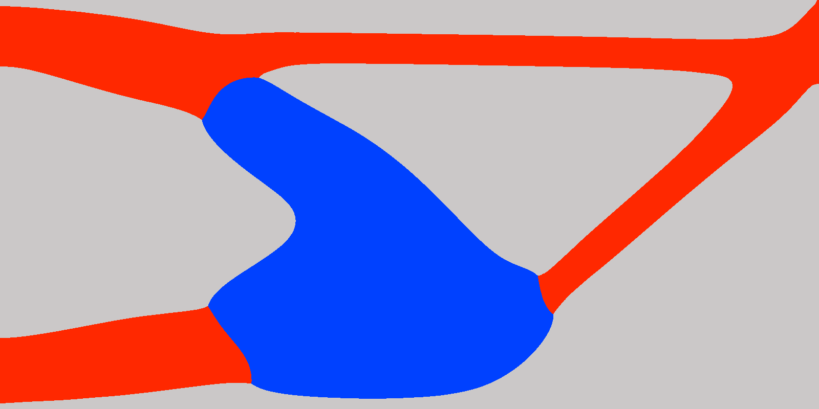
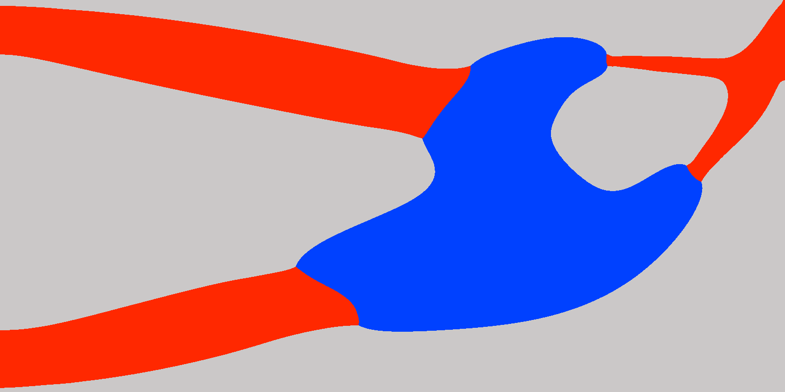
The intermediate results and optimal configurations in Cases 17, 18, and 19 are shown in Figs. 16–18, respectively, and Fig. 19 shows the obtained optimal structures and deformation diagrams in each case. As the virtual springs had large spring constants, the movements in the middle panels of Fig. 19 are barely noticeable. The right panels of Fig. 19 are the deformation diagrams without the virtual springs, i.e., with stiffness values of $({k^{\text{in}}}_{xx},{k^{\text{in}}}_{xy},{k^{\text{in}}}_{yx},{k^{\text{in}}}_{yy})=(0,0,0,0)$ and $({k^{\text{out}}}_{xx},{k^{\text{out}}}_{xy},{k^{\text{out}}}_{yx},{k^{\text{out}}}_{yy})=(0,0,0,0)$ .

In all cases, the optimal configurations were smooth and clear. The non-cavity regions and regions of other structural materials were similarly shaped for different numbers of materials ( $M$ = 2, 3, 4). The regions occupied by the structural materials formed 5 components; 2 “ $>$ ” shaped parts in the left, a beam connected to the output port, and 2 rods in the center which connect the beam and “ $>$ ” shaped parts. These elements are connected by a constricted shape, and there is no hinge-like structure that connects the elements at a single point. The values of the objective functions in Cases 17, 18, and 19 were $-6.46\times 10^{-20},-5.31\times 10^{-20}$ and $-5.19\times 10^{-11}$ , respectively. The upper volume constraints were mostly satisfied (volume constraint functions $<10^{-3}$ ) and the values of the objective functions were negative, indicating successful optimization with a pulling force at the left-side output port. As the virtual springs were arranged at the input and output ports to ensure sufficient strength of the structures, the output parts were hardly deformed in reality (Figs. 19 19, 19, and 19). When the springs were removed and the inputs were applied, the output parts were deformed to the left, as intended (Figs. 19 19, 19, and 19).

5.3 Two-dimensional mean compliance and moment of inertia minimization problems

In this subsection, the proposed optimization method is applied to the two-dimensional mean compliance and moment of inertia minimization problem. Fig. 20 shows the fixed design domain, rotation axis, and boundary conditions in the simulation. The characteristic length $L$ was set to 1 m.

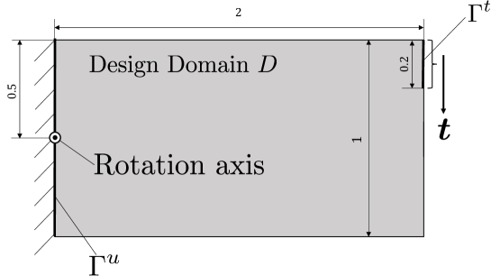
No material was assumed at the fixed displacement boundary $\Gamma^{u}$ , material 1 was assumed at the boundary $\Gamma^{t}$ subjected to the traction force $\bm{t}$ , and material 0 was assumed at the other boundaries.

In these examples, material 2 was assigned half the density of material 1 and material 0 had negligible mass density; that is, we set $(\rho_{0},\rho_{1},\rho_{2})=(0,2,1)$ . The upper limits of the volume constraint $({V^{\text{max}}}_{0},{V^{\text{max}}}_{1},{V^{\text{max}}}_{2})$ were set to (100%, 20%, 20%) of the volume of the fixed design domain. The initial values of the X-LS functions $\phi_{ij}$ were set to 0, and the regularization parameter $\tau_{ij}$ was set to $1\times 10^{-3}$ . We varied the weighting factor $w$ in Eq. (33), which modulates the effects of minimizing the moment of inertia and the compliance, and compared the resulting optimal configurations. The weighting factors were set to $5\times 10^{-13},5\times 10^{-14}$ and $5\times 10^{-15}$ in Cases 20, 21, and 22, respectively. The optimal configurations are shown in Fig. 21.

In Cases 20, 21, and 22, the values of the objective functions were $3.61\times 10^{-11},2.13\times 10^{-11}$ , and $2.08\times 10^{-11}$ , respectively, and the values of the objective functions of moment of inertia $J_{\text{I}}$ defined in Eq. (33) were $7.49\times 10^{1},1.30\times 10^{2}$ , and $1.42\times 10^{2}$ , respectively. The upper volume constraints were mostly satisfied ( $<10^{-10}$ in Case 20 and 21 and $2\times 10^{-3}$ in Case 22). The optimal structure exhibited a smooth boundary. As the weighting coefficient increased, the dense material moved closer to the axis of rotation, thus reducing the moment of inertia $J_{\text{I}}$ . This result was deemed physically reasonable.

5.4 Three-dimensional mean compliance minimization problems

The practicality of the method was evaluated on the mean-compliance minimization problem of a three-dimensional mechanical component. Fig. 22 shows the fixed design domain $D$ (gray region), the nondesign domain (red areas), and the boundary conditions. The characteristic length $L$ was set to 25 mm.

Also in these examples, the isotropic linear elastic materials has Young’s modulus shown in Table 1 and Poisson’s ratio $0.3$ . Material 1 is assigned to the non-design domain. In the following figures of the optimization results, each material region is represented by a color as shown in the Table 1. Except for the Case 25 bellow, among the boundaries of the design domain, Material 1 is specified at the boundary with the non-design domain and material 0 is specified at the other boundaries. For the Case 25, among the boundaries of the design domain, Material 1 is specified at the boundary with the non-design domain, no material is specified at the z-minimum and z-maximum plane and material 0 is specified at the other boundaries. The boundary conditions of the level set functions are set based on the Eq. (7). Since the problem settings are symmetrical about the central plane in the z-axis direction, we analyzed half of the region using the symmetry condition. Initial values of X-LS functions $\phi_{ij}$ is set to 0.

The Young’s moduli of the isotropic linear elastic materials in these examples are listed in Table 1 and the Poisson’s ratio was 0.3. The nondesign domain was composed of material 1. The following figures show the optimization results. The material colors in these results are those assigned in Table 1. In all cases, material 1 was assumed at the boundary with the nondesign domain and material 0 was assumed at the other boundaries. In Case 25 alone, no material was assumed at the z-minimum and z-maximum plane. As the problem settings were symmetric about the central plane in the z-axis direction, only half of the region was analyzed. The X-LS functions $\phi_{ij}$ were initialized to 0.

5.4.1 Examples for $M=3,4$

We first optimized the structures in the cases of three and four materials (Cases 23 and 24, respectively). Case 23 included materials 0, 1, and 2 and Case 24 included Materials 0, 1, 2, and 3 (see Table 1). The maximum volume ratios were set to $({V^{\text{max}}}_{0},{V^{\text{max}}}_{1},{V^{\text{max}}}_{2})$ = (100%, 20%, 20%) in Case 23 and $({V^{\text{max}}}_{0},{V^{\text{max}}}_{1},{V^{\text{max}}}_{2},{V^{\text{max}}}_{3})$ = (100%, 13.3%, 13.3%, 13.3%) in Case 24. The regularization parameter $\tau_{ij}$ was set to $1\times 10^{-4}$ . The optimal configurations in Cases 23 and 24 are presented in Figs. 24 and 23, respectively.

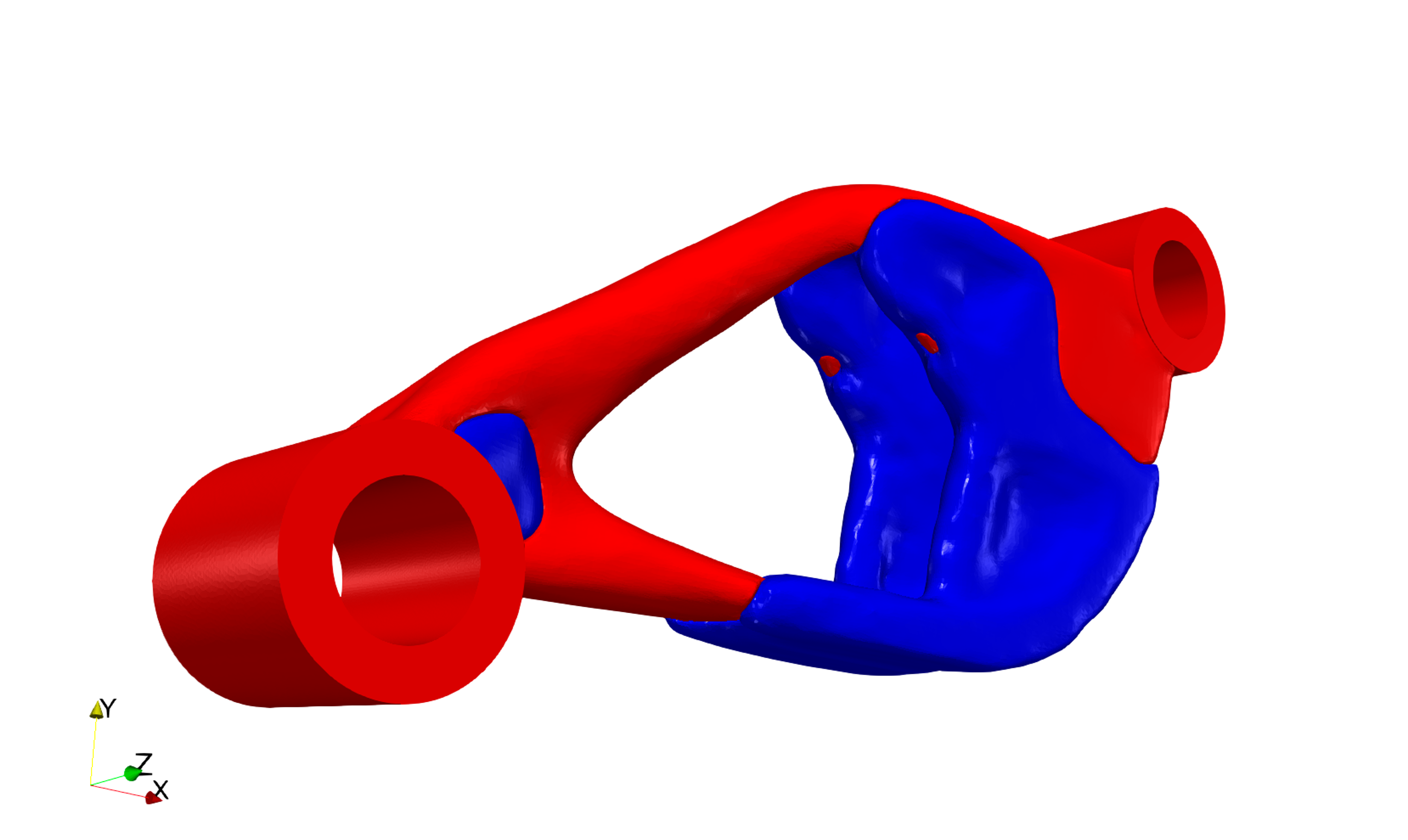
The values of the objective functions in Cases 23 and 24 were $0.190$ . The upper volume constraints were mostly satisfied (volume constraint function $<10^{-5}$ in Case 23 and $<10^{-4}$ in Case 24). In the two optimal structures, the strong material was located near the fixed displacement boundary; the upper right, lower left, and central regions, where the stiffness contribution was low, were hollow. This configuration was compatible with structural mechanics. In addition, the lack of geometrically complex structures, such as checkerboard patterns, indicated that the regularization was properly applied.

5.4.2 Uniform cross-section surface and piecewise linear surface constraints

Similar to the two-dimensional compliance minimization problem, we next imposed uniform cross-section surface constraints and piecewise-linear surface constraints on configurations with three materials (materials 0, 1, and 2 in Table 1). The regularization parameter $\tau_{ij}$ was set to $1\times 10^{-4}$ . In Cases 25–28, we imposed uniform cross-section surface constraints and set the anisotropic regularization parameters $\tilde{\tau}_{ijk}$ as presented in Table 4.

Table 4: Anisotropic regularization parameters

\tilde{\tau}_{ijk}

in cases 25–28

Case	$\tilde{\tau}_{01x}$	$\tilde{\tau}_{01y}$	$\tilde{\tau}_{01z}$	$\tilde{\tau}_{02x}$	$\tilde{\tau}_{02y}$	$\tilde{\tau}_{02z}$	$\tilde{\tau}_{12x}$	$\tilde{\tau}_{12y}$	$\tilde{\tau}_{12z}$
23	1	1	1	1	1	1	1	1	1
25	1	1	$10^{3}$	1	1	$10^{3}$	1	1	$10^{3}$
26	1	1	1	1	1	1	1	1	$10^{3}$
27	1	1	1	1	1	1	$10^{6}$	1	$10^{3}$
28	1	1	1	1	1	1	1	$10^{5}$	$10^{5}$

The normalization coefficients were set to $({K^{\text{ucss}}}_{01},{K^{\text{ucss}}}_{02},{K^{\text{ucss}}}_{12})=(1,1,1)$ in Cases 25 and 26, and $(1,1,10)$ in Cases 27 and 28. In Case 25, the cross-section surface was assumed constant along the z-axis, like cookie cutters. In this problem setting, if material 0 is assumed on the front and back boundary surfaces of the design domain, the entire design domain will be material 0. Therefore, in Case 25 (but not in the other three-dimensional cases), the level set function was set to the Neumann condition $\bm{n}\cdot\nabla\phi_{ij}=0$ at the front and back boundaries of the design domain. In Case 26, the interface between the regions of materials 1 and 2 was constrained to be constant along the z-axis. In Cases 27 and 28, the surface was constrained to be flat, and the uniform cross-section surface constraint was imposed in the direction parallel to the x- and z-axes and parallel to the y- and z-axes, respectively. The optimal configurations in Cases 25–28 are displayed in Figs. 26 – 29.

The values of the objective functions in Cases 25, 26, 27, and 28 were 0.192, 0.190, 0.191, and 0.190, respectively. The upper volume constraints were mostly satisfied (volume constraint functions $<10^{-4}$ in Cases 25, 27, 28 and $<10^{-8}$ in Case 26). In Case 25 (see Fig. 26 26), the uniform cross-section surface constraint was satisfied both at the exterior surface (the boundary between the cavity and other structural material regions) and at the boundary between materials 1 and 2, as evidenced by the coincidence of the front and cross-sectional views in panels 26 and 26 of Fig. 26, respectively. In Case 26, the uniform cross-section surface constraint was not satisfied at the exterior surface (boundary between the cavity and the other structural material regions; see Fig. 27 27) but was satisfied at the boundary between materials 1 and 2, as evidenced by the coincidental front view in panel 27 and sectional view in panel 27 of Fig. 27. In Cases 27 and 28, we confirmed that our method can successfully impose uniform cross-section surface constraints in two directions. In particular, the red and blue regions corresponding to materials 1 and 2, respectively, were divided by planes spanning the entire design domain parallel to the x-z plane in Case 27 (Fig. 28) and to the y-z plane in Case 28 (Fig. 29). These results indicate that the proposed method can selectively constrain the cross-sectional surface between two materials to be uniform in the three-dimensional case.

In Cases 29 and 30, we imposed the piecewise-linear boundary constraints in two directions, that is, we imposed piecewise-linear surface constraints. The piecewise anisotropic regularization parameters $\tilde{\tau}_{ijk}^{{}^{\prime}}$ were set as shown in Table 5.

Table 5: Piecewise anisotropic regularization parameters

\tilde{\tau}_{ijk}^{{}^{\prime}}

in Cases 29 and 30

Case	$\tilde{\tau}_{01x}^{{}^{\prime}}$	$\tilde{\tau}_{01y}^{{}^{\prime}}$	$\tilde{\tau}_{01z}^{{}^{\prime}}$	$\tilde{\tau}_{02x}^{{}^{\prime}}$	$\tilde{\tau}_{02y}^{{}^{\prime}}$	$\tilde{\tau}_{02z}^{{}^{\prime}}$	$\tilde{\tau}_{12x}^{{}^{\prime}}$	$\tilde{\tau}_{12y}^{{}^{\prime}}$	$\tilde{\tau}_{12z}^{{}^{\prime}}$
29	1	1	1	1	1	1	$10^{6}$	1	$10^{3}$
30	1	1	1	1	1	1	1	$10^{5}$	$10^{5}$

The normalization coefficients were set to $\left({K^{\text{ucss}}}_{01},{K^{\text{ucss}}}_{02},{K^{\text{ucss}}}_{12}\right)\\ =(1,1,10)$ . In Cases 29 and 30, the piecewise-linear boundary constraint was imposed parallel to the x- and z-axes and to the y- and z-axes, respectively. The optimal configurations in Cases 29 and 30 are presented in Figs. 30 and 31, respectively.

The values of the objective functions in Cases 29 and 30 were 0.192 and 0.190, respectively. The upper volume constraints were mostly satisfied (volume constraint functions $<5\times 10^{-3}$ in Case 29 and $10^{-4}$ in Case 30). We confirmed that our method successfully imposed linear boundary constraints; that is, the boundary surfaces between materials 1 and 2 were parallel to the x-z plane in Case 29 (see Fig. 30) and to the y-z plane in Case 30 (Fig. 31). Under the uniform cross-section surface constraint, materials 1 and 2 were divided by planes over the entire design domain. The piecewise-linear boundary constraints allow boundaries to be displaced or lost if their cross sections cross the cavity region. In fact, in the optimal structure of Case 29, the two boundaries between the red and blue regions on the right side were higher than the boundary on the left side (see Fig. 30 30). In Case 30, a red region appeared in the upper center but not in the lower center (Fig. 31 31). These results indicate that the proposed method can impose a piecewise-linear boundary constraint in the three-dimensional case.

6 Conclusion

In this paper, we extended the level set method to multiple phases and applied the proposed method to the multi-material topology optimization problem. The study results are summarized below.

1.

We proposed an extended level set method for multiphase representation. For $M$ materials, the proposed method defines $M(M-1)$ level set functions. The boundary between materials $i$ and $j$ is expressed as the zero level set of the level set function $\phi_{ij}$ $(i,j\in\{0,1,\ldots,M-1\},~{}j\neq i)$ .
2.

Based on the extended level set method, we formulated a multi-material topology optimization problem. The proposed method provides a high degree of freedom during the optimization. The topological derivatives are expressed in a simple form.
3.

Optimization procedures for the extended level set method were provided and implemented numerically. To apply the ersatz material approach to multiple materials, the characteristic functions of multi-materials were approximated and smoothed.
4.

Several numerical examples were provided. We first applied the multi-material optimization method to two-dimensional compliance minimization, compliant mechanism optimization, and moment-of-inertia minimization problems using 2–9 different materials. In all numerical examples, the obtained optimal solutions were considered mechanically reasonable, validating the proposed method. We then introduced regularization parameters and examined their effects. It was shown that the proposed method can control the geometric complexity of the boundary between two materials for each combination of two materials. Finally the proposed method was validated using three-dimensional problems.

The shortcomings of the proposed method are described below.

1.

Due to the large number of level set functions, which are design variables, compared to other multi-material representation methods, a large amount of computation time is required to update them and calculate the characteristic functions. It could be improved by parallelization or by omitting the calculation of the part where the material is fixed.
2.

In the proposed method, there are degrees of freedom where the three boundaries should meet at a single point, but they are displaced. Therefore, there is a problem that some regions are not in either phase. In this paper, we formulate an approximate assignment of such a region to one of the phases. This approximation is only heuristic, and its validity is not guaranteed. We cannot exclude the possibility that the approximation may not hold in the process of calculation. The vector-valued level set method can be seen as a solution to this problem by placing constraints between the design variables. However, these constraints are not necessarily essential constraints. One possible solution is to perform optimization with necessary and sufficient constraints.

Acknowledgment

Funding: This work was supported by JST FOREST Program (Grant Number JPMJFR202J, Japan).

The authors would like to thank Enago (www.enago.jp) for the English language review.

Appendix A Extended Level Set Method as a Generalization of Conventional Methods

In this section, we explain that some of the existing multi-phase representation methods based on the level set method are special cases of the X-LS method. For each method, we first describe the concept of the methods and formulate the multiphase representation. We then give some constraint equations for the level set function in the X-LS method. Finally, we rewrite the multiphase representation of the X-LS method using the constraint equations and show that the constrained X-LS representation is equivalent to multiphase representation in the existing method.

A.1 Color level set method

ColorLS method is a multiphase representation method, which represents $2^{n}$ phases with $n$ level set functions, in a principle similar to combining colors from the three primary colors. Fig. 32 shows an example of multiphase representation using the ColorLS method. For simplicity, we consider the case with $M=2^{2}$ . To express each phase, we introduce $n=2$ level set functions, ${\phi^{\text{ColorLS}}}_{0}$ and ${\phi^{\text{ColorLS}}}_{1}$ . We consider that ${\phi^{\text{ColorLS}}}_{0}$ is positive in the gray and red regions (Phases 0 and 1, respectively) and negative in the blue region (Phase 2). Meanwhile, ${\phi^{\text{ColorLS}}}_{1}$ is positive in the gray and blue regions (Phases 0 and 2, respectively) and negative in the red region (Phase 1). The boundary between Phases 0 and 1 is the zero isosurface of the level set function ${\phi^{\text{ColorLS}}}_{1}=0$ . Similarly, the boundary between Phases 0 and 2 is the isosurface of ${\phi^{\text{ColorLS}}}_{0}=0$ and that between Phases 1 and 2 is the isosurface of ${\phi^{\text{ColorLS}}}_{0}=0$ and ${\phi^{\text{ColorLS}}}_{1}=0$ .

In terms of these level set functions, the characteristic functions are expressed as follows:

	$\displaystyle\psi_{0}=H({\phi^{\text{ColorLS}}}_{0})H({\phi^{\text{ColorLS}}}_{1}),$		(54)
	$\displaystyle\psi_{1}=H({\phi^{\text{ColorLS}}}_{0})(1-H({\phi^{\text{ColorLS}}}_{1})),$		(55)
	$\displaystyle\psi_{2}=(1-H({\phi^{\text{ColorLS}}}_{0}))H({\phi^{\text{ColorLS}}}_{1}),$		(56)
	$\displaystyle\psi_{3}=(1-H({\phi^{\text{ColorLS}}}_{0}))(1-H({\phi^{\text{ColorLS}}}_{1})).$		(57)

In the X-LS framework, this material representation is covered by imposing the following constraints on the X-LS function $\phi_{ij}$ :

	$\displaystyle\phi_{20}=\phi_{31}=\phi_{21}={\phi^{\text{ColorLS}}}_{0},$		(58)
	$\displaystyle\phi_{10}=\phi_{32}=\phi_{30}={\phi^{\text{ColorLS}}}_{1}.$		(59)

Material representation in the X-LS method is then transformed as

$\displaystyle\psi_{0}$	$\displaystyle=\prod_{i\neq 0}H(\phi_{i0})$
	$\displaystyle=H({\phi^{\text{ColorLS}}}_{1})H({\phi^{\text{ColorLS}}}_{0})H({\phi^{\text{ColorLS}}}_{1})$
	$\displaystyle=H({\phi^{\text{ColorLS}}}_{0})H({\phi^{\text{ColorLS}}}_{1}),$	(60)
$\displaystyle\psi_{1}$	$\displaystyle=\prod_{i\neq 1}H(\phi_{i1})$
	$\displaystyle=H(-{\phi^{\text{ColorLS}}}_{1})H({\phi^{\text{ColorLS}}}_{0})H({\phi^{\text{ColorLS}}}_{0})$
	$\displaystyle=H({\phi^{\text{ColorLS}}}_{0})(1-H({\phi^{\text{ColorLS}}}_{1})),$	(61)
$\displaystyle\psi_{2}$	$\displaystyle=\prod_{i\neq 2}H(\phi_{i2})$
	$\displaystyle=H(-{\phi^{\text{ColorLS}}}_{0})H(-{\phi^{\text{ColorLS}}}_{0})H({\phi^{\text{ColorLS}}}_{1})$
	$\displaystyle=(1-H({\phi^{\text{ColorLS}}}_{0}))H({\phi^{\text{ColorLS}}}_{1}),$	(62)
$\displaystyle\psi_{3}$	$\displaystyle=\prod_{i\neq 3}H(\phi_{i3})$
	$\displaystyle=H(-{\phi^{\text{ColorLS}}}_{1})H(-{\phi^{\text{ColorLS}}}_{0})H(-{\phi^{\text{ColorLS}}}_{1})$
	$\displaystyle=(1-H({\phi^{\text{ColorLS}}}_{0}))(1-H({\phi^{\text{ColorLS}}}_{1})).$	(63)

Thus, the representation of the characteristic function by X-LS under the constraints given by Eq. (59) is equivalent to material representation by the ColorLS method. Therefore, the ColorLS method is a special case of the X-LS method when $M=4$ . The same is true for $M\geq 5$ , although the demonstration is omitted because the formula is very complex.

A.2 Piecewise-constant level set method

In the PCLS approach [36], each material phase is represented as the corresponding integer values of the PCLS function $\phi^{\text{PCLS}}$ , and the boundaries are described as discontinuities in the PCLS function. Fig. 33 shows the concept of PCLS. The gray, red, and blue regions are the domains of Phases 0, 1, and 2, respectively, in which the piecewise-constant values of the PCLS function $\phi^{\text{PCLS}}$ are 0, 1, and 2, respectively.

The PCLS representation of $M$ material phases is given as

\displaystyle\phi^{\text{PCLS}}=k\quad\text{in}\quad\Omega_{k},\quad k=0,1,\ldots,M-1

(64)

where $\Omega_{k}$ is the domain of Phase $k$ .

In terms of the PCLS function, the characteristic function $\psi_{m}$ can be expressed as follows:

\displaystyle\psi_{k}=H(\phi^{\text{PCLS}}+0.5-k)\{1-H(\phi^{\text{PCLS}}-0.5-k)\},

(65)

with piecewise constant constraints;

\displaystyle\prod_{k=0}^{M-1}(\phi^{\text{PCLS}}-k)=0,

(66)

where $H$ is the Heaviside function defined by Eq. (3).

Here, we constrain the X-LS functions by the following equations.

	$\displaystyle\phi_{ij}+i=\phi^{\text{PCLS}}-0.5\quad\text{if}\quad j>i,$		(67)
	$\displaystyle\prod_{k=0}^{M-1}(\phi_{01}+0.5-k)=0.$		(68)

The phase representation by the X-LS method then transforms as

$\displaystyle\psi_{k}$	$\displaystyle=\prod_{i\neq k}H(\phi_{ik})$
	$\displaystyle=\left(\prod_{i<k}H(\phi_{ik})\right)\left(\prod_{i>k}H(-\phi_{ki})\right)$
	$\displaystyle=\left(\prod_{i<k}H(\phi^{\text{PCLS}}-i-0.5)\right)\left(\prod_{i>k}H(-(\phi^{\text{PCLS}}-k-0.5))\right)$
	$\displaystyle=H(\phi^{\text{PCLS}}-(k-1)-0.5)\{1-H(\phi^{\text{PCLS}}-k-0.5)\}$
	$\displaystyle=H(\phi^{\text{PCLS}}-k+0.5)\{1-H(\phi^{\text{PCLS}}-k-0.5)\}.$	(69)

Thus, the representation of the characteristic functions using the X-LS method under constraints Eq. (68) is equivalent to the representation of the characteristic functions using the PCLS method. Therefore, the PCLS method is a special case of the X-LS method.

A.3 Multi-material level set method

The MMLS method [29, 23, 24] sequentially represents $M$ phases by multiplying $M-1$ sets of level set functions. The MMLS method is conceptualized in Fig. 34. The gray, red, and blue regions in this figure are assigned to Phases 0, 1, and 2, respectively. In the Phase 0 region, the level set function ${\phi^{\text{MMLS}}}_{0}$ is negative and the level set function ${\phi^{\text{MMLS}}}_{1}$ takes any value. In the Phase 1 and 2 regions, the level set function ${\phi^{\text{MMLS}}}_{0}$ is positive and the level set function ${\phi^{\text{MMLS}}}_{1}$ is negative and positive, respectively. The dashed and solid lines in Fig. 34 represent the zero isosurfaces coincident and not coincident with the actual phase boundaries, respectively. The boundary between Phase 0 and the other phases is the zero isosurface of the level set function ${\phi^{\text{MMLS}}}_{0}=0$ . Meanwhile, the boundary between Phases 1 and 2 is the zero isosurface of the level set function ${\phi^{\text{MMLS}}}_{1}=0$ .

In the MMLS method, the characteristic function $\psi_{m}$ of each material $m$ can be expressed as follows:

	$\displaystyle\psi_{0}=1-H({\phi^{\text{MMLS}}}_{1}),$		(70)
	$\displaystyle\psi_{k}=(1-H({\phi^{\text{MMLS}}}_{k}))\prod^{k-1}_{i=0}H({\phi^{\text{MMLS}}}_{i})\quad(k=1,\ldots,M-1),$		(71)
	$\displaystyle\psi_{M}=\prod^{M-1}_{i=0}H({\phi^{\text{MMLS}}}_{i}).$		(72)

Here, we impose the following constraints on the level set function in the X-LS method:

\displaystyle\phi_{i(i+1)}=\phi_{i(i+2)}=\ldots=\phi_{iM}={\phi^{\text{MMLS}}}_{i}\quad(i=0,1,\ldots,M-1).

(73)

The material representation using X-LS then transforms as follows:

$\displaystyle\psi_{0}$	$\displaystyle=\prod_{i\neq 0}H(\phi_{i0})$
	$\displaystyle=\prod_{i\neq 0}H(-{\phi^{\text{MMLS}}}_{0})$
	$\displaystyle=(H(-{\phi^{\text{MMLS}}}_{0}))^{M-1}$
	$\displaystyle=H(-{\phi^{\text{MMLS}}}_{0})$
	$\displaystyle=1-H({\phi^{\text{MMLS}}}_{0}),$	(74)
$\displaystyle\psi_{k}$	$\displaystyle=\prod_{i\neq k}H(\phi_{ik})$
	$\displaystyle=(\prod_{i=0}^{k-1}H({\phi^{\text{MMLS}}}_{i}))(\prod_{i=k+1}^{M}H(-{\phi^{\text{MMLS}}}_{k}))$
	$\displaystyle=H(-{\phi^{\text{MMLS}}}_{k})\prod_{i=0}^{k-1}H({\phi^{\text{MMLS}}}_{i})$
	$\displaystyle=(1-H({\phi^{\text{MMLS}}}_{k}))\prod_{i=0}^{k-1}H({\phi^{\text{MMLS}}}_{i}),$	(75)
$\displaystyle\psi_{M}$	$\displaystyle=\prod_{i\neq M}H(\phi_{iM})$
	$\displaystyle=\prod_{i=0}^{M-1}H({\phi^{\text{MMLS}}}_{i}).$	(76)

Thus, the representation of the characteristic function using the X-LS method under constraints Eq. (73) is equivalent to the phase representation using MMLS. Therefore, MMLS is a special case of X-LS.

A.4 Vector-valued level set method

The VVLS method defines an $M-1$ dimensional vector-valued function in a domain $D$ and an $M-1$ dimensional level set vector space divided into $M$ subregions corresponding to the $M$ phases. The phase of each point $\bm{x}\in D$ corresponds to the subregion of the level set vector space, in which the vector value of the VVLS function of that point $\bm{\phi}^{\text{VVLS}}(\bm{x})$ exists.

Fig. 35 illustrates the VVLS method for $M=3$ . The gray, red, and blue regions in the upper panel represent Phases 0, 1, and 2, respectively, and the lower panel shows the $M-1=2$ -dimensional vector space. The gray, red, and blue regions are the subregions of the level set vector space corresponding to Phases 0, 1 and 2, respectively. The regions are separated by straight lines that intersect at the origin of the vector space. The vector $\bm{n}_{ij}$ is the normal vector of the boundary between the regions corresponding to phases $i$ and $j$ . As these region boundaries are arbitrarily set, we set their normal vectors as $\bm{n}_{01}=-\bm{n}_{10}=(-1,0)^{T},\bm{n}_{02}=-\bm{n}_{20}=(0,-1)^{T},\bm{n}_{12}=-\bm{n}_{21}=(1,-1)^{T}$ . Thus, in the upper panel of Fig. 35, the value of the inner products of the VVLS function and the normal vectors are as follows:

	$\displaystyle\begin{cases}\bm{n}_{10}\cdot\bm{\phi}^{\text{VVLS}}>0\\ \bm{n}_{20}\cdot\bm{\phi}^{\text{VVLS}}>0\\ \end{cases}\quad\text{in}\quad\Omega_{0},$		(77)
	$\displaystyle\begin{cases}\bm{n}_{01}\cdot\bm{\phi}^{\text{VVLS}}>0\\ \bm{n}_{21}\cdot\bm{\phi}^{\text{VVLS}}>0\\ \end{cases}\quad\text{in}\quad\Omega_{1},$		(78)
	$\displaystyle\begin{cases}\bm{n}_{02}\cdot\bm{\phi}^{\text{VVLS}}>0\\ \bm{n}_{12}\cdot\bm{\phi}^{\text{VVLS}}>0\\ \end{cases}\quad\text{in}\quad\Omega_{2}.$		(79)

In the upper panel of Fig. 35, the boundary between the domains of Phases 0 and 1 is the zero isosurface of the first element of the VVLS function $\phi^{0}_{\text{VVLS}}=0$ . Meanwhile, the boundary between the domains of Phases 0 and 2 is the zero isosurface of the second element of the VVLS function $\phi^{1}_{\text{VVLS}}=0$ and the boundary between Phases 1 and 2 is the zero isosurface of the inner product of the normal vector and level set function, i.e., $\bm{n}_{12}\cdot\bm{\phi}^{\text{VVLS}}=0$ .

In the VVLS method, the characteristic function $\psi_{k}$ is expressed as follows:

\displaystyle\psi_{k}=\prod_{i\neq k}H(\bm{n}_{ik}\cdot\bm{\phi}^{\text{VVLS}})\quad(k=0,\ldots,M-1).

(80)

Here, we consider using phases number is $M=3$ and giving the following equations as constraints, in which ${\phi^{\text{VVLS}}}_{l}$ are considered as intervening variables, for the level set function in the X-LS method.

Assuming three phases (i.e., $M=3$ ), we impose the following constraint equations on the X-LS method, where ${\phi^{\text{VVLS}}}_{l}$ are considered as intervening variables:

\displaystyle\phi_{ij}=\bm{n}_{ij}\cdot\bm{\phi}^{\text{VVLS}},

(81)

where the vectors $\bm{n}_{ij},\bm{\phi}^{\text{VVLS}}$ are defined as follows:

	$\displaystyle\bm{n}_{01}=-\bm{n}_{10}=(-1,0)^{T},$		(82)
	$\displaystyle\bm{n}_{02}=-\bm{n}_{20}=(0,-1)^{T},$		(83)
	$\displaystyle\bm{n}_{12}=-\bm{n}_{21}=(1,-1)^{T},$		(84)
	$\displaystyle\bm{\phi}^{\text{VVLS}}=({\phi^{\text{VVLS}}}_{0},{\phi^{\text{VVLS}}}_{1})^{T}.$		(85)

The material representation by X-LS then transforms as

	$\displaystyle\psi_{k}$	$\displaystyle=\prod_{i\neq k}H(\phi_{ik})$
		$\displaystyle=\prod_{i\neq k}H(\bm{n}_{ik}\cdot\bm{\phi}^{\text{VVLS}}).$		(86)

Thus, the representation of the characteristic functions using the X-LS method under constraints given by Eq. (81) is equivalent to the material representation using VVLS. Therefore, VVLS is a special case of X-LS when $M=3$ . The same holds for $M\geq 4$ but the demonstration is omitted because the formula is very complex.

In conclusion, the proposed method is the most general extension of the level set method for multiphase representation.

References

[1] L. A. Vese, T. F. Chan, A multiphase level set framework for image segmentation using the mumford and shah model, International journal of computer vision 50 (3) (2002) 271–293.
[2] B. Merriman, J. K. Bence, S. J. Osher, Motion of multiple junctions: A level set approach, Journal of Computational Physics 112 (2) (1994) 334–363.
[3] O. Sigmund, S. Torquato, Design of materials with extreme thermal expansion using a three-phase topology optimization method, Journal of the Mechanics and Physics of Solids 45 (6) (1997) 1037–1067.
[4] M. P. Bendsøe, N. Kikuchi, Generating optimal topologies in structural design using a homogenization method, Computer methods in applied mechanics and engineering 71 (2) (1988) 197–224.
[5] M. P. Bendsøe, Optimal shape design as a material distribution problem, Structural optimization 1 (4) (1989) 193–202.
[6] J. A. Sethian, A. Wiegmann, Structural boundary design via level set and immersed interface methods, Journal of computational physics 163 (2) (2000) 489–528.
[7] G. Allaire, F. Jouve, A.-M. Toader, Structural optimization using sensitivity analysis and a level-set method, Journal of computational physics 194 (1) (2004) 363–393.
[8] T. Yamada, K. Izui, S. Nishiwaki, A. Takezawa, A topology optimization method based on the level set method incorporating a fictitious interface energy, Computer Methods in Applied Mechanics and Engineering 199 (45) (2010) 2876–2891.
[9] O. Sigmund, K. Maute, Topology optimization approaches, Structural and Multidisciplinary Optimization 48 (6) (2013) 1031–1055.
[10] H. Emmendoerfer Jr, E. A. Fancello, Topology optimization with local stress constraint based on level set evolution via reaction–diffusion, Computer Methods in Applied Mechanics and Engineering 305 (2016) 62–88.
[11] H. Emmendoerfer Jr, E. A. Fancello, E. C. N. Silva, Level set topology optimization for design-dependent pressure load problems, International Journal for Numerical Methods in Engineering 115 (7) (2018) 825–848.
[12] H. Emmendoerfer Jr, E. A. Fancello, E. C. N. Silva, Stress-constrained level set topology optimization for compliant mechanisms, Computer Methods in Applied Mechanics and Engineering 362 (2020) 112777.
[13] T. Yamada, K. Izui, S. Nishiwaki, A level set-based topology optimization method for maximizing thermal diffusivity in problems including design-dependent effects, Journal of Mechanical Design 133 (3).
[14] H. A. Jahangiry, A. Jahangiri, Combination of isogeometric analysis and level-set method in topology optimization of heat-conduction systems, Applied Thermal Engineering 161 (2019) 114134.
[15] H. Isakari, K. Kuriyama, S. Harada, T. Yamada, T. Takahashi, T. Matsumoto, A topology optimisation for three-dimensional acoustics with the level set method and the fast multipole boundary element method, Mechanical Engineering Journal 1 (4) (2014) CM0039–CM0039.
[16] H. Isakari, T. Kondo, T. Takahashi, T. Matsumoto, A level-set-based topology optimisation for acoustic–elastic coupled problems with a fast bem–fem solver, Computer Methods in Applied Mechanics and Engineering 315 (2017) 501–521.
[17] D. Lanznaster, P. B. de Castro, H. Emmendoerfer, P. Mendonça, E. C. Silva, E. A. Fancello, A level-set approach based on reaction–diffusion equation applied to inversion problems in acoustic wave propagation, Inverse Problems 37 (2) (2021) 025009.
[18] M. Otomori, T. Yamada, K. Izui, S. Nishiwaki, J. Andkjær, A topology optimization method based on the level set method for the design of negative permeability dielectric metamaterials, Computer Methods in Applied Mechanics and Engineering 237 (2012) 192–211.
[19] M. Jung, N. Heo, J. Park, J. Yoo, Multi-directional cloaking structure design using topology optimization, Journal of Electromagnetic Waves and Applications 35 (8) (2021) 1008–1019.
[20] K. Yaji, T. Yamada, M. Yoshino, T. Matsumoto, K. Izui, S. Nishiwaki, Topology optimization using the lattice boltzmann method incorporating level set boundary expressions, Journal of Computational Physics 274 (2014) 158–181.
[21] G. Fujii, Y. Akimoto, Dc carpet cloak designed by topology optimization based on covariance matrix adaptation evolution strategy, Optics letters 44 (8) (2019) 2057–2060.
[22] G. Fujii, Y. Akimoto, Optimizing the structural topology of bifunctional invisible cloak manipulating heat flux and direct current, Applied Physics Letters 115 (17) (2019) 174101.
[23] M. Cui, H. Chen, J. Zhou, A level-set based multi-material topology optimization method using a reaction diffusion equation, Computer-Aided Design 73 (2016) 41–52.
[24] N. Kishimoto, K. Izui, S. Nishiwaki, T. Yamada, Optimal design of electromagnetic cloaks with multiple dielectric materials by topology optimization, Applied Physics Letters 110 (20) (2017) 201104.
[25] M. Noda, Y. Noguchi, T. Yamada, Multi-material topology optimization based on symmetric level set function using the material definition with perfect symmetric property, Transactions of the JSME (in Japanese) 87 (896) (2021) 20–00412–20–00412.
[26] P. Wei, M. Y. Wang, Piecewise constant level set method for structural topology optimization, International Journal for Numerical Methods in Engineering 78 (4) (2009) 379–402.
[27] Z. Luo, L. Tong, J. Luo, P. Wei, M. Y. Wang, Design of piezoelectric actuators using a multiphase level set method of piecewise constants, Journal of Computational Physics 228 (7) (2009) 2643–2659.
[28] M. Y. Wang, X. Wang, “color” level sets: a multi-phase method for structural topology optimization with multiple materials, Computer Methods in Applied Mechanics and Engineering 193 (6-8) (2004) 469–496.
[29] Y. Wang, Z. Luo, Z. Kang, N. Zhang, A multi-material level set-based topology and shape optimization method, Computer Methods in Applied Mechanics and Engineering 283 (2015) 1570–1586.
[30] P. Gangl, A multi-material topology optimization algorithm based on the topological derivative, Computer Methods in Applied Mechanics and Engineering 366 (2020) 113090.
[31] M. Bonnet, G. Delgado, The topological derivative in anisotropic elasticity, Quarterly Journal of Mechanics and Applied Mathematics 66 (4) (2013) 557–586.
[32] S. M. Giusti, A. Ferrer, J. Oliver, Topological sensitivity analysis in heterogeneous anisotropic elasticity problem. theoretical and computational aspects, Computer Methods in Applied Mechanics and Engineering 311 (2016) 134–150.
[33] B. S. Lazarov, M. Schevenels, O. Sigmund, Robust design of large-displacement compliant mechanisms, Mechanical sciences 2 (2) (2011) 175–182.
[34] F. Hecht, New development in freefem++, Journal of numerical mathematics 20 (3-4) (2012) 251–266.
[35] A. Tovar, N. M. Patel, G. L. Niebur, M. Sen, J. E. Renaud, Topology optimization using a hybrid cellular automaton method with local control rules, Journal of Mechanical Design 128 (2006) 1205–1216.
[36] J. Lie, M. Lysaker, X.-C. Tai, A variant of the level set method and applications to image segmentation, Mathematics of computation 75 (255) (2006) 1155–1174.

Extended level set method: a multiphase representation with perfect symmetric property, and its application to multi material topology optimization