Exponentially Stable Adaptive Control of MIMO Systems with Unknown Control Matrix

The theory of Model Reference Adaptive Control (MRAC) was developed in the late 1950s as an approach for efficient and safe aircraft control under the condition of significant parameter uncertainty (Tao, 2003; Dydek et al., 2010; Annaswamy and Fradkov, 2021). Despite the difficulties, which were faced at the initial stage (Dydek et al., 2010), the basic MRAC principles were approved by the engineers over time and found real practical applications in aircraft engineering as well as in other branches of industry (Narendra and Monopoli, 2012). However, many of the conventional assumptions of the classical MRAC paradigm are still not fully relaxed to this day. This keeps the scientific community interested in the improvement of some aspects of this theory (Annaswamy and Fradkov, 2021; Tao, 2014).

In this research, we consider the requirement to know some a priori information about the control input (allocation) matrix $B$ for the implementation of the conventional adaptive laws of the form $\Gamma e_{ref}^{\rm{T}}Pf\left(B\right)$.

It is well known (Tao, 2003, 2014) that, in order to be implementable, such adaptive laws require to know either the control allocation matrix $f\left(B\right)=B$, its sign $f\left(B\right)={\rm{sgn}}\left(B\right)$ or $f\left(B\right)=B_{0}sign(\Lambda)$ for a matrix case. It is rather restrictive for a number of practical scenarios. Therefore, there have been some attempts (Narendra and Kudva, 1974; Reish and Chowdhary, 2014; Roy et al., 2017; Gerasimov et al., 2018; Glushchenko et al., 2021a, 2022) to minimize such a priori needed data about matrix $B$ for MRAC schemes.

In (Tao, 2003; Narendra and Kudva, 1974) conditions are stated, under which the substitution $f\left(B\right)={B_{ref}}$ is allowed, where ${B_{ref}}$ is the input matrix of the reference model. The method in (Narendra and Kudva, 1974) leads to a modified control law, which provides only local stability, and requires knowledge of the lower bound of the determinant of the feedforward controller parameter matrix due to the need for its inversion. The identification-based approach $f\left(B\right)=\hat{B}$ , which is proposed by (Reish and Chowdhary, 2014), does not require any a priori information about the matrix $B$, but needs the plant state matrix $A$ to be known instead. This is an even more restrictive assumption for most applications. (Roy et al., 2017), inspired by (Reish and Chowdhary, 2014), have proposed a combined adaptive control scheme, in which the minimum singular value of the matrix $B$ is assumed to be known. The advantages of (Reish and Chowdhary, 2014; Roy et al., 2017) in comparison with the previous solutions (Tao, 2003; Narendra and Kudva, 1974) are the relaxation of the regressor persistent excitation (PE) requirement, which is used in (Tao, 2003; Narendra and Kudva, 1974), for the exponential stability of the control scheme and parameter convergence. The method in (Roy et al., 2017) includes a nonlinear operator, which prevents singularity when the controller parameters matrices are inverted. However, the finiteness of the number of switches in the course of the adaptation has not been rigorously proved for such an operator, and as a consequence, the chattering is possible.

Considering the adaptive output feedback control problem, the method, which is based on the dynamic regressor extension and mixing (DREM) procedure (Aranovskiy et al., 2016), is proposed in (Gerasimov et al., 2018). It guarantees no more than one switch of the nonlinear operator under the condition of a known lower bound of the high-frequency gain. Later this approach has been improved and applied to the problem of the state feedback control of the multi-input multi-output (MIMO) systems in (Glushchenko et al., 2021a), in which it is also guaranteed that no more than one switch is required. Such a method needs the lower bound value of the determinant of the control allocation matrix. In (Glushchenko et al., 2022), considering single-input single-output (SISO) systems, another direct adaptive law is proposed, which is based on the I-DREM procedure (Glushchenko et al., 2021b). It does not require any a priori information about $B$ and guarantees the exponential stability of the closed-loop system if the regressor is finitely exciting (FE).

The present paper is an attempt to extend the result of (Glushchenko et al., 2022) to the case of MIMO systems. The main scientific contribution of the research is threefold: 1) an adaptive control scheme for unknown MIMO plants without any a priori knowledge about system matrices is obtained; 2) the exponential stability of the closed-loop control system is guaranteed when the vector of signals (states and controls) measured from the plant is finitely exciting (FE); 3) the monotonicity of transients of all control law matrices elements is provided. To the best of the authors’ knowledge, properties 1-3 are provided simultaneously for the first time.

The paper is organized as follows. Section II presents a problem statement. Section III contains the main result. Section IV is to analyze the control system stability. The numerical experiments are presented in Section V.

Notation. $\lvert{.}\rvert$ is the absolute value, $\lVert{.}\rVert$ is the Euclidean norm of a vector, $\lambda_{\min}\left(.\right)$ and $\lambda_{\max}\left(.\right)$ are the matrix minimum and maximum eigenvalues, respectively, $vec\left(.\right)$ stands for the matrix vectorization. $I_{n\times n}$, $0_{n\times n}$ and $1_{n\times n}$ are identity, zero and ones $n\times n$ matrices, respectively. We also use the fact that for all (possibly singular) ${n\times n}$ matrices $M$ the following holds: $adj\{M\}M=det\{M\}I_{n\times n}$. The following definition from (Tao, 2003) is also used.

Definition 1. The regressor $\varphi\left(t\right)$ is finitely exciting $\left({\varphi\left(t\right)\in{\rm{FE}}}\right)$ over $\left[{t_{r}^{+};\;{\rm{}}{t_{e}}}\right]$ if there exist ${t_{e}}>t_{r}^{+}\geq 0$ and $\alpha>0$ such that the following holds

where $\alpha$ is the excitation level.

Let the corollary of Theorem 9.4 from (Tao, 2003) be introduced.

Corollary 1. For any matrix $D>0$, a Hurwitz matrix $A\in{\mathbb{R}^{n\times n}}$, a matrix $B$ such that a pair $(A,B)$ is controllable there exists a matrix $P=P^{\rm{T}}>0$, a scalar $\mu>0$ and matrices $Q{\rm{,}}\;K$ of appropriate dimension such that:

Let the problem of adaptive state feedback control of the linear time-invariant (LTI) MIMO systems be considered:

where $x\left(t\right)\in{\mathbb{R}^{n}}$ is the measurable state vector, ${x_{0}}\in{\mathbb{R}^{n}}$ is the known (or possibly unknown) vector of initial conditions, ${u\left(t\right)}\in{\mathbb{R}^{m}}$ is a control vector, ${A}\in{\mathbb{R}^{n\times n}}$ is the state matrix, ${B}\in{\mathbb{R}^{n\times m}}$ is the control (allocation) matrix of full column rank. The pair $\begin{pmatrix}A,\;B\end{pmatrix}$ is controllable. The vector ${\Phi\left(t\right)}\in{\mathbb{R}^{n+m}}$ is considered to be measurable at each time instant $t>0$, whereas ${\theta_{AB}}\in{\mathbb{R}^{\left({n+m}\right)\times n}}$ is time-invariant and unknown.

The reference model, which is used to define the required control quality for (3), is described as:

where ${x_{ref}\left(t\right)}\in{\mathbb{R}^{n}}$ is the reference model state vector, ${x_{0ref}}$ is the initial conditions vector, $r\left(t\right)\in{\mathbb{R}^{m}}$ is the reference, ${A_{ref}}\in{\mathbb{R}^{n\times n}}$ is the Hurwitz state matrix of the reference model, ${B_{ref}}\in{\mathbb{R}^{n\times m}}$ is the input matrix.

The matching condition is supposed to be met for the plant (3) and the reference model (4).

Assumption 1. There exist ${K_{x}}\in{\mathbb{R}^{m\times n}}$ and ${K_{r}}\in{\mathbb{R}^{m\times m}}$ such that the following holds:

Considering (5), the control law for (3) is chosen as:

where ${\hat{K}_{x}}\left(t\right)\in{\mathbb{R}^{m\times n}}$ and ${\hat{K}_{r}}\left(t\right)\in{\mathbb{R}^{m\times m}}$ are adjustable parameters and ${\hat{K}_{r}}\left(0\right)\neq{0_{m\times m}}$.

Having substituted (6) into (3) and subtracted (4) from the obtained equation, the following error equation is written:

Here ${e_{ref}\left(t\right)}\!\buildrel\Delta\over{=}\!x\left(t\right)\!-\!{x_{ref}\left(t\right)}{\rm{,}}\;{\tilde{K}_{x}}\left(t\right)\!\buildrel\Delta\over{=}\!{\hat{K}_{x}}\left(t\right)\!-\!{K_{x}}{\rm{,}}\;{\tilde{K}_{r}}\left(t\right)\buildrel\Delta\over{=}\linebreak\buildrel\Delta\over{=}{\hat{K}_{r}}\left(t\right)-{K_{r}}$. The following notation is introduced in (7):

where $\omega\left(t\right)\in{\mathbb{R}^{n+m}}$, $\hat{\theta}\in{\mathbb{R}^{\left({n+m}\right)\times m}}$ is the vector of the control law adjustable parameters.

Considering (8) and the difference between the initial conditions for (3) and (4), the equation (7) is written as:

The objective is formulated on the basis of (9).

Goal. When $\Phi\left(t\right)\in{\rm{FE}}$, it is required to hold:

where $\xi\left(t\right)={\begin{bmatrix}{e_{ref}^{\rm{T}}}\left(t\right)&{ve{c^{\rm{T}}}\left({\tilde{\theta}\left(t\right)}\right)}\end{bmatrix}^{\rm{T}}}\in{\mathbb{R}^{n+m\left({n+m}\right)}}$ is the augmented tracking error.

The main result of this study is based on the direct self-tuning regulators concept. Having $\Phi\left(t\right)$ at hand, it is proposed to apply some mathematical transformations to $\left(\ref{eq3}\right)$ and, using the obtained results, derive the measurable regression equation with the help of $\left(\ref{eq5}\right)$:

where $\Delta\left(t\right)\!\in\!{\mathbb{R}},\;y_{\theta}\!\left(t\right)\!\in\!{\mathbb{R}^{\left({n+m}\right)\times m}}$ are measurable signals.

Applying the results of (Glushchenko et al., 2022, 2021b), Corollary 1 and conditions of the exponential stability, it is proposed to derive the adaptive law for $\hat{\theta}\left(t\right)$ on the basis of $\left(\ref{eq11}\right)$, which guarantees that $\left(\ref{eq10}\right)$ holds when $\Phi\left(t\right)\in{\rm{FE}}$.

The subsection $3.1$ of this section contains the description of steps to obtain the regression equation $\left(\ref{eq11}\right)$, under the condition that the plant $\left(\ref{eq3}\right)$ matrices are unknown and $\dot{x}\left(t\right)$ is unmeasurable. The subsection $3.2$ presents the adaptive law, which ensures that $\left(\ref{eq10}\right)$ is achieved and does not require a priori knowledge of the plant $\left(\ref{eq3}\right)$ matrices.

According to (Glushchenko et al., 2021b), the adaptive law (20) provides exponential convergence of the parameter error $\tilde{\theta}\left(t\right)$ only. In the following theorem we formulate strict formal conditions, under which the law (20) guarantees that the objective (10) is met.

Theorem 1. Let $\Phi\left(t\right)\in{\rm{FE}}$, then, if $\gamma$ value is chosen according to

then the adaptive law (20) ensures that:

1. 1.

   $\forall{t_{a}}\geq{t_{b}}\;\;{\rm{}}\left|{{{\tilde{\theta}}_{i}}\left({{t_{a}}}\right)}\right|\leq\left|{{{\tilde{\theta}}_{i}}\left({{t_{b}}}\right)}\right|{\rm{;}}$

2. 2.

   $\forall t\geq t_{r}^{+}\;\;{\rm{}}\xi\left(t\right)\in{L_{\infty}}{\rm{;}}$

3. 3.

   $\forall t\geq{t_{e}}$ the error $\xi$ converges exponentially to zero at the rate, which minimum value is directly proportional to the parameters ${\gamma_{0}}\geq 1$ and ${\gamma_{1}}\geq 0$.

Proof of Theorem is presented in Appendix.

Thus, in contrast to existing approaches (Tao, 2014; Narendra and Kudva, 1974; Reish and Chowdhary, 2014; Roy et al., 2017; Gerasimov et al., 2018; Glushchenko et al., 2021a, 2022), when $\gamma$ is chosen according to (21), the adaptive law (20) does not require any a priori information about the matrices of the system (3) and guarantees that the objective (10) is fulfilled. Some additional technical details of the law (20) implementation can be found in (Glushchenko et al., 2022).

Remark 2. When $\Phi\left(t\right)\in{\rm{FE}}$, the switching of the nonlinear operator (21) may occur only once, since, according to Proposition 1, $\Omega\left(t\right)$ is a positive semidefinite function.

Remark 3. The condition $\Phi\left(t\right)\in{\rm{FE}}$ is necessary but not sufficient to achieve (10). According to Assumption 2 and Remark 1, the necessary and sufficient conditions are $\overline{\varphi}\left(t\right)\in{\rm{FE}}$ and Assumption 2. This may become a dramatically critical requirement for some applications.

Remark 4. In contrast to the baseline direct laws of the form $\Gamma e_{ref}^{\rm{T}}\left(t\right)Pf\left(B\right)$, the proposed one (20) provides stability of ${e_{ref}}\left(t\right)$ only when $\Phi\left(t\right)\in{\rm{FE}}$. Therefore, to implement (20) in practice, the a priori information is required that this condition holds. If $\Phi\left(t\right)\notin{\rm{FE}}$ for a particular plant (3) and a particular reference, then it is possible to hold $\Phi\left(t\right)\in{\rm{FE}}$ artificially by addition of the dither noise to the control or the reference signal according to (Adetola and Guay, 2006; Cao et al., 2007). At the same time, we can not use conventional modular design (Krstic et al., 1995) to ensure stability of the control system when $t<t_{e}$ as neither the sign nor the values of elements of matrix B are known.The actual problem is to obtain conditions on $r\left(t\right)$, under which the requirement $\Phi\left(t\right)\in{\rm{FE}}$ is met for the whole class of MIMO plants (3).

Numerical simulation to test the proposed adaptive control system, which consists of the control law (6), processing procedure (12), (13), (15)-(17), (19), and the adaptive law (20), was conducted using the model of a lateral-directional motion of a conventional small passenger aircraft from (Lavretsky and Wise, 2013):

where $x_{1}$ is the bank angle, $x_{2}$ is the sideslip angle, $x_{3}$ is the roll rate, $x_{4}$ is the vehicle yaw rate, $u_{1}$ is the aileron position, $u_{2}$ is the rudder position. According to the problem statement, all plant (22) parameters and initial conditions were considered as unknown.

The reference model and reference for (22) were also chosen as in (Lavretsky and Wise, 2013):

The parameters of the adaptive law (20), filters (12), operators $\mathfrak{H}\left[.\right]{\rm{,}}\mathfrak{G}\left[.\right]$, and the initial values of the parameters of the control law (6) were picked as follows:

As for practical implications of Assumptions 1 and 2, the plant and reference model had the same structure, all plant equations with parametric uncertainty contained sufficient number of controls, (12) ensured excitation propagation.

Figure 1 shows transient curves of the plant (22) states and ideal ones, which were obtained by setting into the reference model the following plant initial conditions: ${x_{ref}}\left(0\right)=x\left(0\right)$. Figure 2 is to compare the ideal control vector $u^{*}$ and the one $u$ obtained from the proposed adaptive system. Figure 3 demonstrates transients of the controller feedback parameters ${\hat{K}_{x}\left(t\right)}$, whereas Figure 4 – of the feedforward ones ${\hat{K}_{r}}\left(t\right)$. In the figures controller parameters estimates were ”frozen” till $0.15$ s as till that moment $\Delta(t)=0$ because condition (1) had not been satisfied yet ($t_{e}=0.15$ s).

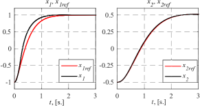
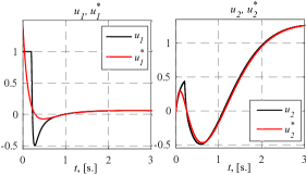
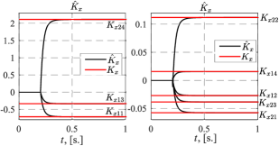
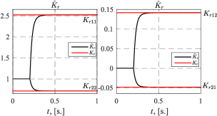
The results of the numerical experiments presented in Figures 1-4 validated the contribution of this work noted in the introduction in comparison with known solutions (Tao, 2014; Narendra and Kudva, 1974; Reish and Chowdhary, 2014; Roy et al., 2017; Gerasimov et al., 2018; Glushchenko et al., 2021a, 2022). They confirmed the theoretical conclusions of Theorem 1, and showed that (10) was achieved.

Important features of the developed system are the monotonicity of each controller parameter adjustment process, and the fact that the rate of the parameter convergence is directly adjustable by choice of scalar parameters $\gamma_{0}$ and $\gamma_{1}$. These improve the transient behavior of states and control vector, and make the commissioning of the developed adaptive system significantly easier.

Considering the unknown MIMO plants, the adaptive state feedback control system has been proposed, which does not require any a priori information about the plant matrices. When the regressor vector $\Phi\left(t\right)$, which is constituted of the plant states and control signals, is finitely exciting, the proposed system guarantees exponential stability of the tracking error, and the exponential convergence of the control law parameters identification error to zero. Considering numerical experiments, the effectiveness of the proposed approach to solve the adaptive control problem of the lateral-directional motion of the conventional small passenger aircraft was demonstrated.

Establishing the conditions, under which $\Phi\left(t\right)$ is FE for any generic MIMO system, is the scope of further research, as well as the plans to extend the obtained results to output-feedback control case.

Proof of Theorem 1. As $\Omega\left(t\right)\in\mathbb{R}$, the solution of (20) is:

As ${\rm{sign}}\left({\gamma{\Omega^{2}\left(t\right)}}\right)={\mathop{\rm const}\nolimits}>0$, then it follows from (A1) that $\left|{{{\tilde{\theta}}_{i}}\left({{t_{a}}}\right)}\right|\leq\left|{{{\tilde{\theta}}_{i}}\left({{t_{b}}}\right)}\right|{\rm{}}\forall{t_{a}}\geq{t_{b}}$. This completes the proof of the first part of the theorem.

As ${A_{ref}}$ is a Hurwitz matrix and $B$ is of full column rank, then according to the corollary of KYP lemma (2), there exist $P{\rm{,}}\;Q{\rm{,}}\;D{\rm{,}}\;K,$ which satisfy (3). Then, the quadratic function to analyze the stability of (9) is chosen:

Applying $tr\left({AB}\right)=BA$, the derivative of (A2) with respect to (9), (20) is written as:

Without the loss of generality, $D$ is chosen so as $K{K^{\rm{T}}}~{}=~{}{K^{\rm{T}}}K={I_{m\times m}}$. Then we have:

Two cases are considered: $t<{t_{e}}$ and $t\geq{t_{e}}$. Firstly, let $t<{t_{e}}$. Following (20) and (21), it holds that $\Omega\left(t\right)=0$ and $\left\|{\tilde{\theta}}\right\|=\left\|{\tilde{\theta}\left(0\right)}\right\|$. Then, $\forall t<{t_{e}}$ (A4) is rewritten as:

A maximum eigenvalue of $\omega\left(t\right){\omega^{\rm{T}}}\left(t\right)$ over $\left[{0{\rm{;}}\;\;{t_{e}}}\right)$ is introduced:

Taking into consideration (A6), the equation (A5) for $t<{t_{e}}$ is rewritten as:

where ${\eta_{\rm{1}}}={\rm{min}}\left\{{{\textstyle{{\mu{\lambda_{{\rm{min}}}}\left(P\right)}\over{{\lambda_{{\rm{max}}}}\left(P\right)}}}{\rm{;2}}}\right\}{\rm{;}}\;\;{r_{B}}=\left({\delta+1}\right){\left\|{\tilde{\theta}\left(0\right)}\right\|^{2}}$.

Having solved (A7), it is obtained:

As ${\lambda_{\mathop{\rm m}\nolimits}}{\left\|\xi\right\|^{2}}\leq V$ and $V\left(0\right)\leq{\lambda_{M}}{\left\|{\xi\left(0\right)}\right\|^{2}}$, then we obtain from (A8) that the estimate of $\xi\left(t\right)$ is bounded for $\forall t<{t_{e}}$:

Secondly, let $t\geq{t_{e}}$. Considering (21) and that $\forall t\geq{t_{e}}$ $0\!<\!{\Omega_{{\rm{LB}}}}\!\leq\!\Omega\left(t\right)\!\leq\!{\Omega_{{\rm{UB}}}}$ holds, we obtain from (21) $\forall t\geq{t_{e}}$:

It holds for any $\omega\left(t\right)$ that:

So (A10) is written as:

where ${\eta_{\rm{2}}}={\rm{min}}\left\{{{\textstyle{{\mu{\lambda_{{\rm{min}}}}\left(P\right)}\over{{\lambda_{{\rm{max}}}}\left(P\right)}}}{\rm{;\;\;2}}\left({\kappa+{\gamma_{1}}}\right)}\right\}.$

The inequality (A12) is solved, and it is obtained for $t\geq{t_{e}}$:

Considering ${\lambda_{\mathop{\rm m}\nolimits}}{\left\|\xi\right\|^{2}}\leq V$, $V\left({{t_{e}}}\right)\leq{\lambda_{M}}{\left\|{\xi\left({{t_{e}}}\right)}\right\|^{2}}$ and (A9), the estimate of $\xi\left(t\right)$ for $t\geq{t_{e}}$ is obtained from (A13):

References

• Adetola and Guay (2006) Adetola, V. and Guay, M. (2006). Excitation signal design for parameter convergence in adaptive control of linearizable systems. In Proc. of IEEE Conf. Decis. Control, 447–452. San Diego, CA.
• Annaswamy and Fradkov (2021) Annaswamy, A. and Fradkov, A. (2021). A historical perspective of adaptive control and learning. Annual Reviews in Control, 52, 18–41.
• Aranovskiy et al. (2016) Aranovskiy, S., Bobtsov, A., Ortega, R., and Pyrkin, A. (2016). Performance enhancement of parameter estimators via dynamic regressor extension and mixing. IEEE Trans. Autom. Control, 62(7), 3546–3550.
• Aranovskiy et al. (2022) Aranovskiy, S., Ushirobira, R., Korotina, M., and Vedyakov, A. (2022). On preserving-excitation properties of dynamic regressor extension scheme. IEEE Trans. Autom. Control. Ieeexplore.ieee.org/abstract/document/9767689.
• Cao et al. (2007) Cao, C., Hovakimyan, N., and Wang, J. (2007). Intelligent excitation for adaptive control with unknown parameters in reference input. IEEE Trans. Autom. Control, 52(8), 1525–1532.
• Chowdhary et al. (2013) Chowdhary, G., Yucelen, T., Muhlegg, M., and Johnson, E. (2013). Concurrent learning adaptive control of linear systems with exponentially convergent bounds. Int. J. of Adapt. Control Signal Process., 27(4), 280–301.
• Dydek et al. (2010) Dydek, Z., Annaswamy, A., and Lavretsky, E. (2010). Adaptive control and the nasa x-15-3 flight revisited. IEEE Control Syst. Mag., 30(3), 32–48.
• Gerasimov et al. (2018) Gerasimov, N., Ortega, R., and Nikiforov, V.O. (2018). Relaxing the high-frequency gain sign assumption in direct model reference adaptive control. Eur. J. Control, 43, 12–19.
• Glushchenko and Lastochkin (2022) Glushchenko, A. and Lastochkin, K. (2022). Exponentially convergent direct adaptive pole placement control of plants with unmatched uncertainty under fe condition. IEEE Control Systems Letters, 6, 2527–2532.
• Glushchenko et al. (2021a) Glushchenko, A., Petrov, V., and Lastochkin, K. (2021a). I-drem mrac with time-varying adaptation rate and no a priori knowledge of control input matrix sign to relax pe condition. In Proc. of Eur. Control Conf., 2175–2180. Rotterdam, Netherlands.
• Glushchenko et al. (2021b) Glushchenko, A., Petrov, V., and Lastochkin, K. (2021b). I-drem: Relaxing the square integrability condition. Autom. Remote Control, 82(7), 1233–1247.
• Glushchenko et al. (2022) Glushchenko, A., Petrov, V., and Lastochkin, K. (2022). Exponentially stable adaptive control. part i. time-invariant plants. Autom. Remote Control, 83, 548–578.
• Korotina et al. (2022) Korotina, M., Romero, J., Aranovskiy, S., Bobtsov, A., and Ortega, R. (2022). A new on-line exponential parameter estimator without persistent excitation. Sys. and Control Lett., 159, 105079.
• Krstic et al. (1995) Krstic, M., Kanellakopoulos, I., and Kokotovic, P. (1995). Nonlinear and Adaptive Control Design. Wiley, New York.
• Lavretsky and Wise (2013) Lavretsky, E. and Wise, K. (2013). Robust adaptive control. Springer, London.
• Narendra and Kudva (1974) Narendra, K. and Kudva, P. (1974). Stable adaptive schemes for system identification and control-part i. IEEE Trans. Syst., Man and Cyber., (6), 542–551.
• Narendra and Monopoli (2012) Narendra, K. and Monopoli, R. (2012). Adaptive Control Design and Analysis. Academic Press, New York.
• Ortega et al. (2021) Ortega, R., Bobtsov, A., and Nikolaev, N. (2021). Parameter identification with finite-convergence time alertness preservation. IEEE Control Syst. Lett., 6, 205–210.
• Reish and Chowdhary (2014) Reish, B. and Chowdhary, G. (2014). Concurrent learning adaptive control for systems with unknown sign of control effectiveness. In Proc. of IEEE Conf. Decis. Control, 4131–4136. Los Angeles, CA.
• Roy et al. (2017) Roy, S., Bhasin, S., and Kar, I. (2017). Combined mrac for unknown mimo lti systems with parameter convergence. IEEE Trans. Autom. Control, 63(1), 283–290.
• Tao (2003) Tao, G. (2003). Adaptive Control Design and Analysis. Wiley, New York.
• Tao (2014) Tao, G. (2014). Multivariable adaptive control: A survey. Automatica, 50(11), 2737–2764.