Exponential Stability and Design of Sensor Feedback Amplifiers for Fast Stabilization of Magnetizable Piezoelectric Beam Equations
Abstract
The dynamic partial differential equation (PDE) model governing longitudinal oscillations in magnetizable piezoelectric beams exhibits exponentially stable solutions when subjected to two boundary state feedback controllers. An analytically established exponential decay rate by the Lyapunov approach ensures stabilization of the system to equilibrium, though the actual decay rate could potentially be improved. The decay rate of the closed-loop system is highly sensitive to the choice of material parameters and the design of the state feedback amplifiers. This paper focuses on investigating the design of state feedback amplifiers to achieve a maximal exponential decay rate, which is essential for effectively suppressing oscillations in these beams. Through this design process, we explicitly determine the safe intervals of feedback amplifiers that ensure the theoretically found maximal decay rate, with the potential for even better rates. Our numerical results reaffirm the robustness of the decay rate within the chosen range of feedback amplifiers, while deviations from this range significantly impact the decay rate. To underscore the validity of our results, we present various numerical experiments.
Intelligent Materials, Distributed Parameter Systems, Feedback Stabilization, Maximal Decay Rate, Lyapunov Approach
1 Introduction
Piezoelectric ceramics, including lead-free materials like barium titanate, sodium potassium niobate, and sodium bismuth titanate, are renowned multifunctional smart materials that generate electric displacement in response to mechanical stress [26]. Their small size and high power density make them ideal for various industrial applications, including implantable biomedical devices [5, 25], wearable interfaces with PVDF sensors [7], biocompatible sensors [32], and ultrasound imagers and cleaners [24]. Their fast response, large mechanical force, and fine resolution contribute to their effectiveness [10].
Consider a piezoelectric beam, clamped on one side and free on the other, with sensors for tip velocity and current. he beam is of length and thickness . Assume that the transverse oscillations of the beam are negligible, so the longitudinal vibrations, in the form of expansion and compression of the center line of the beam, are the only oscillations of note together with the electromagnetic effects. Existing mathematical models often oversimplify intrinsic mechanical or electromagnetic interactions, impacting boundary feedback stabilizability [1, 17, 20, 6, 27, 29].
While electrostatic and quasi-static approaches based on Maxwell’s equations are typically sufficient for non-magnetizable piezoelectric beams, assessing radiated electromagnetic power requires consideration of electromagnetic waves generated by mechanical fields [28]. Therefore, fully dynamic models of piezoelectric beams are essential. Denoting as the longitudinal oscillations and as the total charge accumulated at the electrodes, the equations of motion form following system of partial differential equations [17]
| (7) |
where , , , , and are the mass density per unit volume, the elastic stiffness, the impermeability, the piezoelectric constant, and the magnetic permeability, respectively, and and are strain and voltage actuators, respectively.
Define with , and
| (9) |
Note that and are non-identical and represent significantly different wave propagation speeds in (7). The natural energy of the solutions is defined as
| (12) |
The exact observability result for the model (7) with and with only one sensor measurement is not possible [17]. However, by employing two sensor measurements, (tip velocity) and (total current accumulated at electrodes), a suboptimal observation time is achieved [23]. This result is later refined to include the optimal observation time [21].
Theorem 1
When the observed sensor signals and are amplified and fed back to (7), a closed-loop system is formed. The amplification range depends on the sensor limits. While using only one sensor feedback can make the system energy dissipative, it is insufficient for exponential stabilization in . This is because the closed-loop system with this control design imposes strict conditions on stabilization results [17]. Exponential stability is jeopardized for a large class of material parameters and is only achievable for a small subset [18].
Let be the feedback amplifiers for the two sensor measurements of the closed-loop system and , respectively. The strain and voltage actuators and are chosen to be proportional to the sensor feedback amplifiers,
| (15) |
The exponential stability of the closed-loop system (7), (15) has been studied in [23], where the proof relies on decomposing the system into conservative and dissipative components. However, this method does not explicitly describe the decay rate or allow optimization of the feedback amplifiers.
The primary objective of this paper is to establish the existence of an exponential decay rate for the system described by (7) and (15) through the meticulous construction of a Lyapunov function. Given the impracticality of traditional spectral analysis due to the strong coupling in the wave system, we adopt a multiplier approach combined with an optimization argument to define a safe range of intervals for each feedback amplifier and . This ensures that the decay rate provided by the Lyapunov approach is achievable for any type of initial conditions .
Our methodology provides a maximal decay rate for the system, serving as an upper bound to the optimal decay rate since the actual decay rate could potentially be even better. Existing literature on optimal actuator designs commonly offers different approaches for infinite-dimensional systems [8, 13, 15, 22], and finite-dimensional systems [4, 9]. Our approach is particularly valuable for model reductions by Finite Differences or Finite Elements [21] for (7). Notably, the Lyapunov-based exponential stability proof [2], uniformly as the discretization parameter with the recently proposed order-reduced Finite Differences [12], closely resembles the approach employed here.
2 Exponential Stability Result
For the solutions of the system (7),(15) to stabilize exponentially, the energy must be dissipative. The proof of the following dissipativity theorem is omitted.
Lemma 1
For all the energy in (12) is dissipative. In other words,
Now, let’s define an energy-like functional in order to establish a perturbed energy functional as follows
| (16) | ||||
| (17) |
Here, will be determined as a function of sensor feedback amplifiers and later.
The following two lemmas for and are needed to prove our main exponential stability result. Let
| (18) |
Proof 2.1.
By the Hölder’s, Minkowski’s, Triangle inequalities, as well as algebraic manipulations, satisfies
Since this leads to and analogously, and therefore, (19) is immediate
Lemma 3
For any , in (16) satisfies the following inequalities,
| (22) |
Proof 2.2.
Now, the exponential stability result takes the following form
Theorem 2.
The energy of solutions decays exponentially, i.e. for any ,
| (25) |
| (26) |
3 Optimization of Sensor Feedback Amplifiers
The decay rate in Theorem 2 provides an upper bound for the exponential decay rate of the system. In this section, we provide an optimization process for feedback amplifiers and that ensure the maximal value of , given by
| (29) |
Since and are functions of and the sensor feedback amplifiers and in (15), the following results provide intervals for the feedback amplifiers and that ensures the decay rate (29) is attained.
Theorem 3.
Define non-negative constants
| (30) |
with any such that
| (31) |
Proof 3.1.
Observe that to achieve the in (29), it is sufficient to have and .
Thus, i.e. implies that
| (33) |
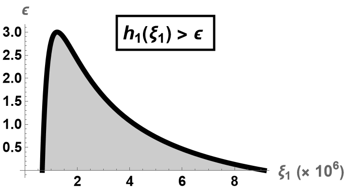
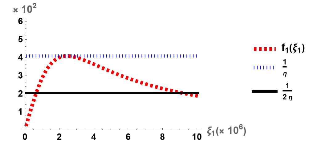
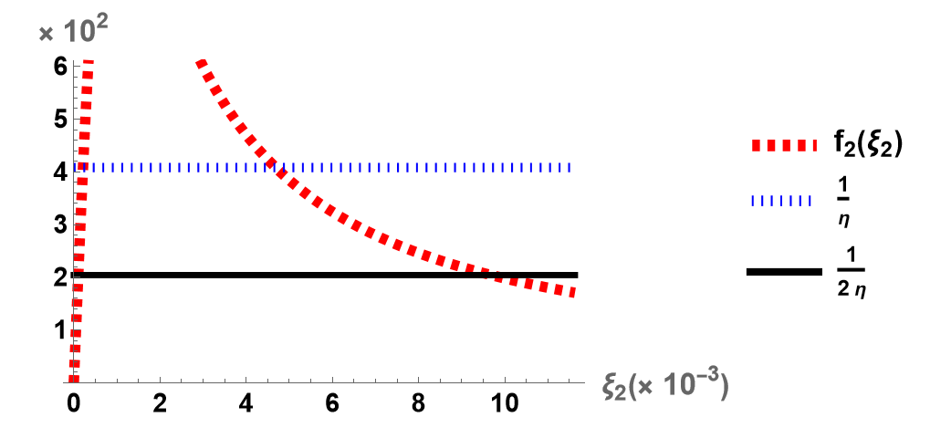
Noting that by (18), defines an upper bound for , and observe that must be chosen in between the following roots of to ensure , see Fig. 1
Observe that if and only if . Seeking the critical points of leads to for which achieves its maximum value. Substituting into (33) yields the following upper bound for
| (35) |
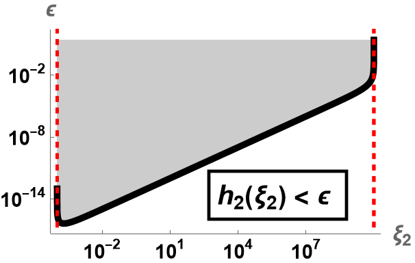
By Since , the denominator is chosen to be strictly positive. This leads to where
| (37) |
and and are the two vertical asymptotes of see dashed lines in Fig. 1. Note that this condition ensures . Seeking the critical points of leads to for which takes its minimum value. Substituting into (33) yields the lower bound for
| (39) |
where by (18). Restricting and in between roots and asymptotes, respectively, values corresponding to the filled regions in Fig. 1 satisfy conditions (35) and (39), respectively.
We prove that such and exist. Note that the sufficient condition for is the existence of satisfying (31) which is ensured by
| (41) |
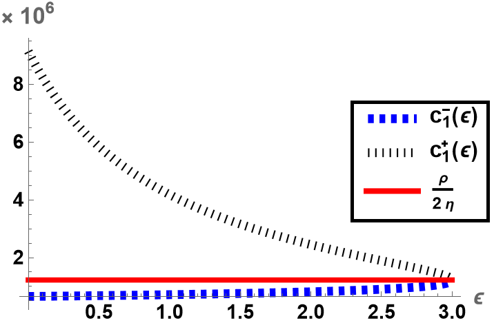
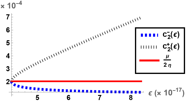
The amplifier maximizing and the amplifier minimizing are always in the respective intervals, i.e. and . Moreover, as approaches to the upper (lower) bound gets smaller (larger) and gets larger (smaller), see Fig. 2. Feedback amplifiers chosen within the intervals ensure that and are satisfied, see Figs. 3 and 4.
4 Simulations and Numerical Experiments
In this section, we present numerical simulations primarily aimed at demonstrating the following:
- •
-
•
Comparison of the reduced model exponential decay rates for a selection of feedback amplifiers.
Moreover, we address a common challenge encountered in standard model reductions, such as Finite Differences (FD) and Finite Elements (FE), which introduce spurious high-frequency vibrational modes to the system. These spurious modes significantly impact the decay rate of the system. In fact, reduced models lack the uniform observability property as the mesh parameter approaches zero, necessitating filtering techniques such as the direct Fourier filtering [3, 11] or the indirect filtering [30].
To mitigate the adverse effects of approximation methods on the decay rate, we consider a recently introduced technique known as Order-Reduced Finite Differences (ORFD) [12]. The ORFD method has been observed to retain the decay rate of the infinite-dimensional system. For rigorous stability analyses of all three approximations, interested readers can refer to [2].
Consider a given natural number , which denotes the number of nodes in the spatial semi-discretization. Let’s introduce the mesh size as , and discretize the interval as Let be the approximation of the solution of (7)-(15) at the point space for any , and let and .
In the ORFD method, in addition to the standard nodes we also consider the in-between middle nodes of each subinterval, denoted by Define the average, and difference operators
| (43) |
It is worth noting that by considering odd-number derivatives at the in-between nodes within the uniform discretization of , higher-order approximations are achieved [12].
The ORFD approximation of equations (7) with (15) is
| (44) |
where and are matrices for material parameters, and is the matrix for the state feedback amplifiers, defined as
the mass matrix is defined by
the central difference matrix is
and the boundary node matrix is a zero matrix except for the -th entry, which is due to the boundary damping being injected at the last node. Here, denotes the matrix Kronecker product. It’s worth noting that equation (44) can be rewritten in the first-order form as
| (45) |
| (46) |
The discretized energy corresponding to (45) is
| (47) |
To show the importance of our analysis for the choices of sensor feedback amplifiers via the optimization process outlined in the previous section, sample numerical simulations are presented for the material constants in Table 1.
| Parameter | Symbol | Value | Unit |
|---|---|---|---|
| Length of the beam | m | ||
| Mass density | kg/ | ||
| Magnetic permeability | H/m | ||
| Elastic stiffness | N/ | ||
| Piezoelectric constant | C/ | ||
| Impermittivity | m/F |
Note that in (29) depends solely on the material parameters. In particular, for the material parameters in Table 1. Letting , which is a valid choice for any system according to equations (41), the intervals for optimal sensor feedback amplifiers in (30), corresponding to are as follows:
| (48) |
Here note that both the maximal decay rate and the corresponding intervals for feedback amplifiers in (48) are independent of the choice of initial conditions.
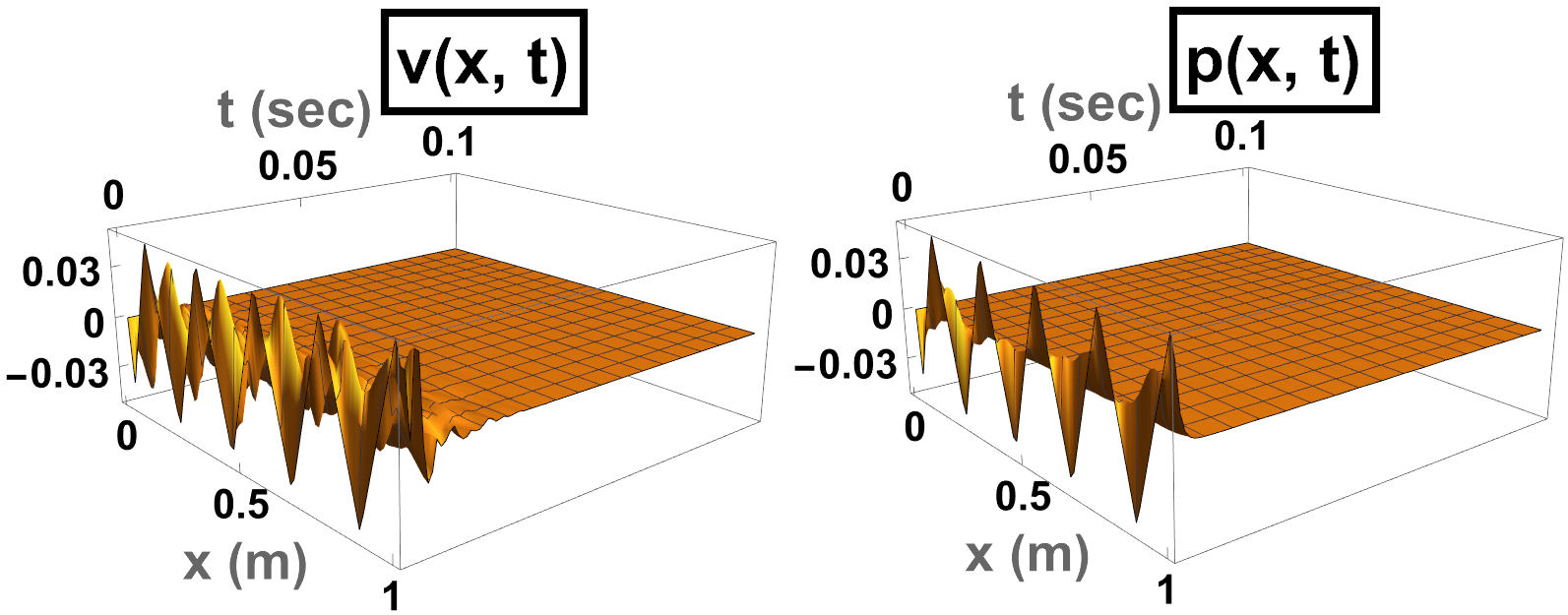
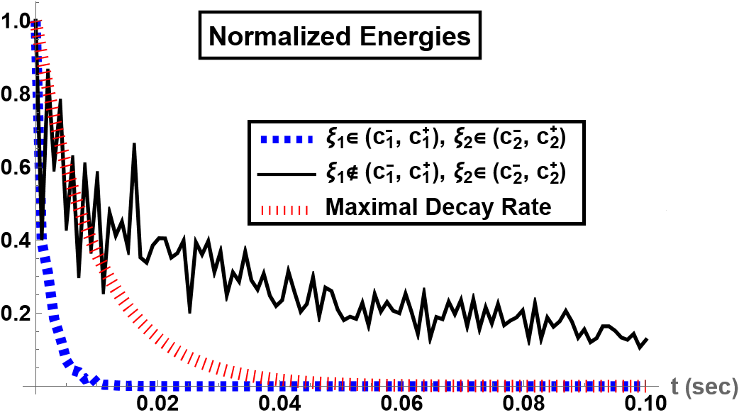
For simulations, we take nodes, and we choose triangular (hat-type) initial conditions that are composed of high and low-frequency vibrational nodes. The simulations are performed for sec to show the rapid exponential decay of solutions. Indeed, the solutions of the system (44) with the choices of optimal feedback amplifiers and , are observed drive all states to zero state rapidly, e.g. see Fig. 5, and the total energy follows the exponentially decay in a higher rate than claimed , Fig. 7.
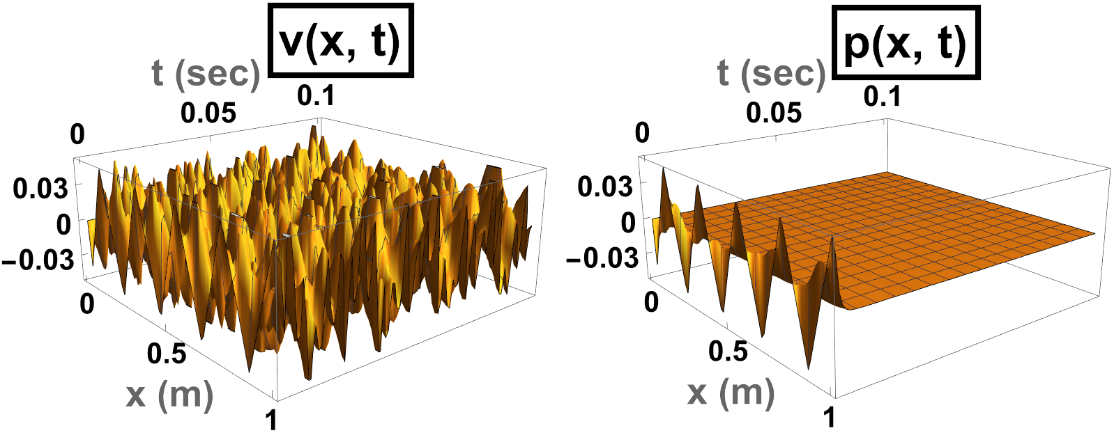
Our analysis indicates that even a relatively small perturbation in the values of the feedback amplifiers can lead to suboptimal performance. Indeed, when and does not fall within the range , the system still continues to exhibit low and high-frequency longitudinal oscillations for seconds, as demonstrated in Figure 6. Furthermore, the energy of the system decays in an unstable manner, with a decay rate significantly larger than , as depicted in Figure 7.
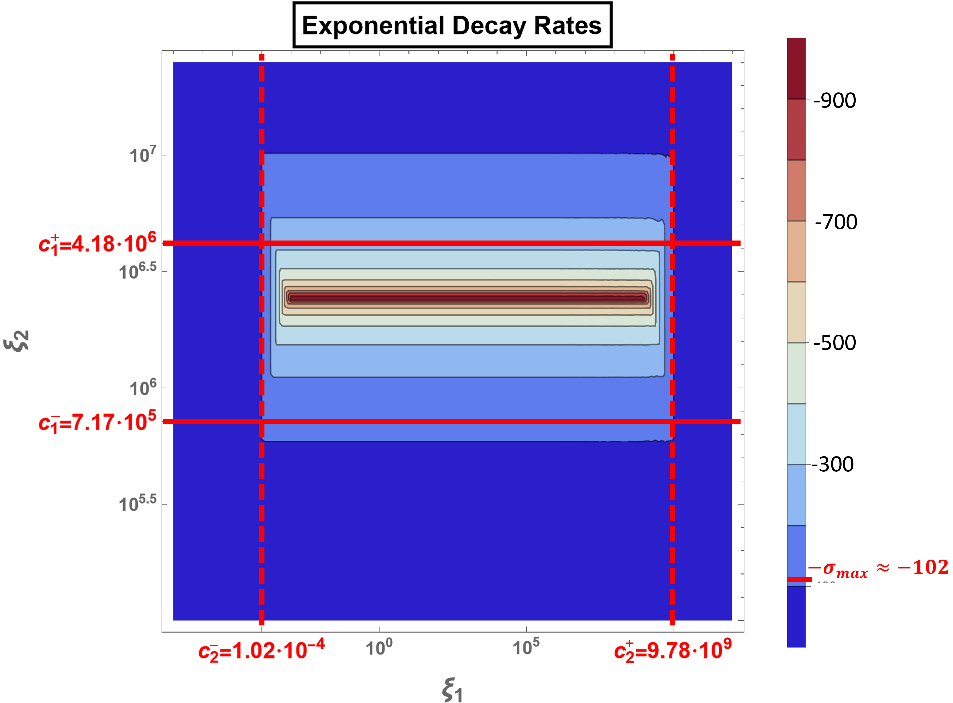
To demonstrate the robustness of our theoretical findings, we examine the spectrum of the numerical approximation. Let denote the eigenvalues of as defined in Equation (46). The decay rate of the system (7) with (15), and the theoretically derived decay rate in Theorem (2), can be approximated as the maximal real part of the eigenvalues of , specifically . A contour plot of in terms of the feedback amplifiers and is presented in Figure 8. It is notable that as the feedback amplifiers and fall within the intervals and , respectively shown as red lines, the maximal decay rate is achieved. Conversely, the decay rate significantly diminishes outside of these intervals. Exact values of for selected feedback amplifiers are also provided in Table 2. As a final note, the decay rates are much smaller than when both feedback amplifiers are chosen from the intervals and .
5 Conclusions & Future Work
In summary, using the Lyapunov approach, we derived the exponential decay rate for system (7), with the design of state feedback amplifiers and as described in (15). This decay rate ensures fast stabilization, though improvements are possible. The rate depends on material parameters and feedback amplifiers. Our numerical results confirm the robustness of this decay rate, with deviations affecting it from the theoretical value. Interactive simulations are available through the Wolfram Demonstrations Project [31].
A full numerical analysis and proof of exponential stability for the semi-discretized model (44), as , and determining optimal designs of feedback amplifiers remain beyond this paper’s scope and are ongoing research. However, the Lyapunov approach here serves as the basis for results in [2], where the discretized model achieves the same decay rate as the PDE model.
Future work can extend these concepts to multi-layer magnetizable piezoelectric beams, which have numerous practical applications [19]. The design of feedback amplifiers may become more delicate when there are more than two state feedback amplifiers, as highlighted in [19]. There is also potential to explore general hyperbolic PDE systems with multiple boundary dampers. Relevant studies address systems with random inputs [14] and the optimal design and placement of actuators in higher-dimensional systems [16, 15], both of which are valuable for future research.
References
- [1] A. K. Aydın, A.Ö Özer, J. Walterman, A Novel Finite Difference-Based Model Reduction and a Sensor Design for a Multilayer Smart Beam With Arbitrary Number of Layers, IEEE Control Syst. Lett., 7 (2023), 1548-553.
- [2] A.Ö. Özer, A.K. Aydin, J. Walterman, A Robust Finite-Difference Model Reduction for the Boundary Feedback Stabilization of Fully-dynamic Piezoelectric Beams, arXiv:2309.07492, under revision, 2023.
- [3] H.E. Boujaoui, H. Bouslous, L. Maniar, Boundary Stabilization for 1-d Semi-Discrete Wave Equation by Filtering Technique Bull. TICMI, 17-1 (2013), 1–18.
- [4] N. Cîndea, A. Münch, A mixed formulation for the direct approximation of the control of minimal -norm for linear type wave equations, Calcolo, 52-3 (2015), 245-288.
- [5] C. Dagdeviren, et al., Recent Progress in Flexible and Stretchable Piezoelectric Devices for Mechanical Energy Harvesting, Sensing and Actuation, Extreme Mech. Lett., 9(1) (2016), 269-281.
- [6] M.C. de Jong, et al., On control of voltage-actuated piezoelectric beam: A Krasovskii passivity-based approach, Eur. J. Control, 69 (2023), 100724.
- [7] W. Dong, et al., Wearable human–machine interface based on PVDF piezoelectric sensor, Trans. Inst. Meas. Control, 39-4 (2017), 398–403.
- [8] I. Ftouhi, E. Zuazua, Optimal design of sensors via geometric criteria, J. Geom. Anal., 33-8 (2023), 253.
- [9] B. Geshkovski, E. Zuazua, Optimal actuator design via Brunovsky’s normal form, IEEE Trans. Autom. Control, (2022) pp. 6641-6650.
- [10] G.Y. Gu, et al., Modeling and Control of Piezo-Actuated Nanopositioning Stages: A Survey, IEEE Trans. Autom. Sci. Eng., 13-1 (2016), 313–332.
- [11] J.A Infante and E. Zuazua, Boundary observability for the space semi-discretizations of the 1-D wave equation, Math. Model. Num. Anal., 33 (1999), 407-438.
- [12] J. Liu, B.Z. Guo, A new semi-discretized order reduction finite difference scheme for uniform approximation of 1-D wave equation, SIAM J. Control Optim., 58 (2020), 2256-2287.
- [13] K. Kunisch, P. Trautmann, B. Vexler, Optimal control of the undamped linear wave equation with measure valued controls, SIAM Journal on Control and Optimization, 2016, 1212-1244.
- [14] F.J. Marín, J. Martínez-Frutos, F. Periago Robust averaged control of vibrations for the Bernoulli-Euler beam equation. Journal of Optimization Theory and Applications. 2017, 174-428.
- [15] K. Morris, M.A. Demetriou, S.D. Yang, Using H2-control performance metrics for the optimal actuator location of distributed parameter systems, IEEE Trans. Autom. Control, 60-2 (2015), 450-462.
- [16] A. Münch, P. Pedregal, F. Periago, Optimal Internal Stabilization of the Linear System of Elasticity. Arch Rational Mech Anal 193 (2009), 171–193.
- [17] K. Morris, A.Ö. Özer, Modeling and stability of voltage-actuated piezoelectric beams with electric effect, SIAM J. Control Optim., 52-4 (2014), 2371-2398.
- [18] A.Ö. Özer, Further stabilization and exact observability results for voltage-actuated piezoelectric beams with magnetic effects, Math. Control Signals Syst., 27 (2015), 219-244.
- [19] A.Ö. Özer, Modeling and controlling an active constrained layered (ACL) beam actuated by two voltage sources with/without magnetic effects, IEEE Trans. Autom. Control, 62-12 (2017), 6445–6450.
- [20] A.Ö. Özer, K.A. Morris, Modeling and related results for current-actuated piezoelectric beams by including magnetic effects, ESAIM: COCV, 26-8 (2019), 1-24.
- [21] A.Ö. Özer, W. Horner, Uniform boundary observability of Finite Difference approximations of non-compactly-coupled piezoelectric beam equations, Appl. Anal., 101-5 (2022), 1571-1592.
- [22] Y. Privat, E. Trélat, E. Zuazua, Actuator design for parabolic distributed parameter systems with the moment method, SIAM J. Control Optim., 55-2 (2017), 1128-1152.
- [23] A.J.A. Ramos, M.M. Freitas, D.S. Almeida Jr., S.S. Jesus, T.R.S. Moura, Equivalence between exponential stabilization and boundary observability for piezoelectric beams with magnetic effect, Z. Angew. Math. Phys., 70-60 (2019).
- [24] Ultrasound imaging of the brain and liver, Science Daily, Acoust. Soc. Am., 26 June 2017.
- [25] Q. Shi, T. Wang, C. Lee, MEMS Based Broadband Piezoelectric Ultrasonic Energy Harvester (PUEH) for Enabling Self-Powered Implantable Biomedical Devices, Sci. Rep., 6 (2016), 24946.
- [26] R.C. Smith, Smart Material Systems, (SIAM, 2005).
- [27] T. Voss, J.M.A. Scherpen, Stabilization and shape control of a 1D piezoelectric Timoshenko beam, Automatica, 47-12 (2011), 2780-85.
- [28] J. Yang, An Introduction to the Theory of Piezoelectricity, Springer, New York, 2005.
- [29] B. Yubo, C. Prieur, Z. Wang, Stabilization of a Rayleigh beam with collocated piezoelectric sensor/actuator. Evol. Equ. Control Theory, (2023).
- [30] L.T. Tebou, E. Zuazua, Uniform boundary stabilization of the finite difference space discretization of the 1-D wave equation. Adv. Comput. Math., 26 (2007), 337-365.
- [31] J. Walterman, A.K. Aydin, A.Ö. Özer, Piezoelectric beam dynamics, Wolfram Demonstrations Project, Published: June 13, 2023.
- [32] H.S. Wang, et al., Biomimetic and flexible piezoelectric mobile acoustic sensors with multiresonant ultrathin structures for machine learning biometrics, Sci. Adv., 7-7 (2021).