This paper was converted on www.awesomepapers.org from LaTeX by an anonymous user.
Want to know more? Visit the Converter page.

Exponential mixing for random nonlinear wave equations:
weak dissipation and localized control

Ziyu Liu, Dongyi Wei, Shengquan Xiang, Zhifei Zhang, Jia-Cheng Zhao School of Mathematical Sciences, Peking University, 100871, Beijing, China. [email protected] School of Mathematical Sciences, Peking University, 100871, Beijing, China. [email protected] School of Mathematical Sciences, Peking University, 100871, Beijing, China. [email protected] School of Mathematical Sciences, Peking University, 100871, Beijing, China. [email protected] School of Mathematical Sciences, Peking University, 100871, Beijing, China. [email protected]
Abstract.

We establish a new criterion for exponential mixing of random dynamical systems. Our criterion is applicable to a wide range of systems, including in particular dispersive equations. Its verification is in nature related to several topics, i.e., asymptotic compactness in dynamical systems, global stability of evolution equations, and localized control problems.

As an initial application, we exploit the exponential mixing of random nonlinear wave equations with degenerate damping, critical nonlinearity, and physically localized noise. The essential challenge lies in the fact that the weak dissipation and randomness interact in the evolution.

Key words and phrases:
Exponential mixing; Nonlinear wave equations; Global stability; Asymptotic compactness; Controllability
2020 Mathematics Subject Classification:
37A25, 37S15, 37L50, 35L71, 93C20.

1. Introduction

The ergodic and mixing properties, crucial for the understanding of random systems, have been the focus of research yielding significant advancements in recent decades [59, 60, 9, 72, 100]. However, there have been few results achieved for dispersive equations. The analysis in this setting is usually delicate in the absence of smoothing effect; the existing criteria valid for parabolic-type equations are hardly applicable.

Does the mixing property hold for general dispersive equations?

We provide a criterion of exponential mixing for random dynamical systems in general Polish space, i.e. Theorem A. This result is an attempt to seek for sharp sufficient conditions for the exponential mixing of dispersive equations, as an affirmative answer to the above question. Especially, the criterion, composed by asymptotic compactness, irreducibility and coupling condition, is closely related to dynamical system, dispersive equations and control theory.

As an initial application of the criterion, we establish the exponential mixing for a general model of nonlinear wave equations in the form

u+a(x)tu+u3=η,\boxempty u+a(x)\partial_{t}u+u^{3}=\eta,

i.e. Theorem B, where a(x)a(x) induces the damping effect, and η\eta stands for the random noise. The generality mentioned encompasses several aspects, including degenerate/localized damping, critical nonlinearity111In the context of nn-dimensional wave equations, the Sobolev-critical exponent of nonlinearity is n/(n2)n/(n-2) for n3n\geq 3 (see, e.g., [3]), which differs from the energy-critical exponent (n+2)/(n2)(n+2)/(n-2) (see, e.g., [10]). This is justified by the Sobolev embedding H1L2n/(n2)H^{1}\hookrightarrow L^{2n/(n-2)}, implying that if a nonlinear function satisfies a polynomial growth with power not exceeding n/(n2)n/(n-2), then its Nemytskiĭ operator maps H1H^{1} into L2L^{2}. While we focus on the cubic nonlinearity that is Sobolev-critical, our results and their proofs should be adaptable to the case of super-cubic nonlinearity. and random noise localized in physical space. In particular, the weak dissipation mechanism induced by the localized damping, mingled with the random perturbations, contributes to part of the main challenges in the research; see Sections 1.2,1.3 later. We believe that the approach is general and adaptable to other types of dispersive equations.

In the sequel, let us give a sketch of those topics involved in the criterion:

  • (1)(1)

    Asymptotic compactness is a fundamental object in the theory of global attractor for dynamical systems, motivated by the issues in turbulence [50, 80]. In this topic the dispersive setting is fairly subtle due to the lack of smoothing effect [3, 64]. In addition, the localization of damping and randomness lead to extra obstacles in our analysis.

  • (2)(2)

    The issue of irreducibility will be reduced to a stability problem, where the latter is a significant topic in the dynamics of dispersive equations [5, 57, 86, 68, 84].

  • (3)(3)

    The coupling condition corresponds to the stabilization which is one of the central problems in control theory [85, 26]. Our analysis of coupling condition involves various objects, including unique continuation, Carleman estimates, Hilbert uniqueness method and the localized dissipation, constituting a long piece of section in this paper.

Below in Section 1.1 we give an overview of the abstract criterion (i.e. Theorem A), including historical backgrounds and main contributions. In Section 1.2 we present the mixing result for the random wave equations (i.e. Theorem B), and discuss its generality. Section 1.3 outlines the proof of Theorem B, highlighting the main challenges and our approaches. A brief outline of the rest of the paper is available in Section 1.4.

1.1. Probabilistic framework

In this section we introduce a new criterion for exponential mixing of random dynamical systems. This criterion is a consequence of inspiration from the prior related frameworks and the observation on asymptotic compactness from the dynamical system point of view. It is applicable to a wide class of dispersive equations.

1.1.1. Historical backgrounds

The study of ergodic and mixing properties for randomly forced equations has been a principal motivation of ergodic theory for Markov processes. In particular, it has led to significant results for the 2D Navier–Stokes systems; for the early achievements; see, e.g., [15, 43, 49, 90, 58, 91, 75, 42]. In recent years, Hairer and Mattingly [59, 60] introduce the asymptotic strong Feller property to provide a first result for the situation when the noise is white in time and is extremely degenerate in Fourier modes. More recently, Kuksin–Nersesyan–Shirikyan [72] propose a controllability property to establish a similar result when the degenerate random forces are coloured in time. The reader is referred to, e.g., [61, 95, 51, 11, 73] for other contributions in the context of extremely degenerate noise. In [100, 102], Shirikyan invokes another controllability approach to study the case in which the random perturbation is localized in the physical space. In the context of unbounded domains, the recent paper [94] by Nersesyan derives exponential mixing by developing the controllability approaches of the papers [72, 102].

There have been several general approaches applied to the ergodic and mixing properties for various models. For instance, Hairer–Mattingly–Scheutzow [63] formulate a generalized form of Harris theorem [65] (see also [93, 62] for a detailed account), providing a criterion for exponential mixing and applying it to stochastic delay equations. We refer the reader to [23, 60, 56] for some applications for stochastic parabolic equations and modifications of the Harris-type results. Another intensively studied approach is the coupling method, developed in [58, 90, 91, 74, 76, 77]. Based on the coupling method, Kuksin and Shirikyan [78, 99] propose general conditions, i.e., recurrence and squeezing, for mixing properties. Some applications and extensions for both ODE and PDE models of such framework can be found in, e.g., [87, 100, 102, 101].

1.1.2. Obstructions for mixing of dispersive equations, an idea from dynamical systems

In the context of dispersive equations, the main difficulty lies in the non-compactness of the resolving operator, which results from the lack of the smoothing effect. This leads to an aftermath that the aforementioned frameworks for mixing properties seem hardly applicable to the dispersive setting. For instance, the squeezing [78] usually requires extra regularity of the target trajectory. Analogous obstacles appear to the discussion of the asymptotic strong Feller property [59], approximate controllability [31, 72], etc. Accordingly, our research starts with a question,

How to compensate for the absent compactness?

Our answering this question employs the notion of asymptotic compactness from the dynamical system theory. Recall that the mixing property describes a certain type of limiting behavior that a physical system asymptotically converges to a statistical equilibrium in the distribution sense. Accordingly, one may relax the compactness requirement and provide an alternative of a limiting form. At the same time, the theory of global attractor for infinite-dimensional dynamical system involves a viewpoint of asymptotic compactness, illustrating such limiting-type compactness [3, 64]. These motivate us to build up an explicit relation between the asymptotic compactness for possibly non-compact semiflow and the mixing property.

1.1.3. A general framework

Let 𝒳\mathcal{X} and 𝒵\mathcal{Z} be Polish spaces, and denote by dd the metric on 𝒳\mathcal{X}. Let S:𝒳×𝒵𝒳S\colon\mathcal{X}\times\mathcal{Z}\rightarrow\mathcal{X} be a continuous mapping, and {ξn;n}\{\xi_{n};n\in\mathbb{N}\} a sequence of 𝒵\mathcal{Z}-valued independent identically distributed (i.i.d. for abbreviation) random variables with a common law \ell. We consider a random dynamical system defined by

xn+1=S(xn,ξn),n,x_{n+1}=S(x_{n},\xi_{n}),\quad n\in\mathbb{N}, (1.1)

with initial condition

x0=x.x_{0}=x. (1.2)

We proceed to describe our abstract result for system {xn;n}\{x_{n};n\in\mathbb{N}\}, omitting some inessential technical details. Assume first that \ell is compactly supported, and the mapping SS is Lipschitz on any bounded set. The essential hypotheses are roughly stated as follows:

  1. (𝐇)\mathbf{(H)}
    1. (a)(a)

      (Asymptotic compactness) There exists a compact subset 𝒴\mathcal{Y} of 𝒳\mathcal{X} such that {xn;n}\{x_{n};n\in\mathbb{N}\} exponentially converges to 𝒴\mathcal{Y} in a pathwise manner. We further denote the attainable set from 𝒴\mathcal{Y} by 𝒴\mathcal{Y}_{\infty} (see Definition 2.1).

    2. (b)(b)

      (Irreducibility) There exists z𝒴z\in\mathcal{Y} with the following property: for every ε>0\varepsilon>0, there is m+m\in\mathbb{N}^{+} and p>0p>0 such that for any x𝒴x\in\mathcal{Y}_{\infty},

      (d(xm,z)<ε)p.\mathbb{P}(d(x_{m},z)<\varepsilon)\geq p.
    3. (c)(c)

      (Coupling condition) For every x,x𝒴x,x^{\prime}\in\mathcal{Y}_{\infty}, the pair (x1,x1)(x_{1},x_{1}^{\prime}) admits a coupling (,)(\mathcal{R},\mathcal{R}^{\prime}) satisfying

      (d(,)>12d(x,x))Cd(x,x),\mathbb{P}(d(\mathcal{R},\mathcal{R}^{\prime})>\tfrac{1}{2}d(x,x^{\prime}))\leq Cd(x,x^{\prime}),

      where x1x_{1}^{\prime} is defined as in (1.1),(1.2) with xx replaced by xx^{\prime}.

It is worth mentioning that the hypotheses of irreducibility and coupling condition are directly inspired by the previous works [61, 42] and [100, 102], respectively. See Section 2 for more information.

The following result is a simplified version of our criterion for exponential mixing. See Section 2.1 for a rigorous description of this criterion, where the hypotheses are more general to some extent.

Theorem A.

Assume that hypothesis (𝐇)\mathbf{(H)} holds. Then the Markov process {xn;n}\{x_{n};n\in\mathbb{N}\}, defined by (1.1),(1.2), has a unique invariant measure μ\mu_{*} on 𝒳\mathcal{X}. Moreover, μ\mu_{*} is exponential mixing, i.e., there exists a constant β>0\beta>0 such that

𝒟(xn)μLC(x)eβn\|\mathscr{D}(x_{n})-\mu_{*}\|_{L}^{*}\leq C(x)e^{-\beta n}

for any x𝒳x\in\mathcal{X} and nn\in\mathbb{N}, where L\|\cdot\|^{*}_{L} denotes the dual-Lipschitz distance on 𝒳\mathcal{X} and 𝒟(xn)\mathscr{D}(x_{n}) stands for the law of xnx_{n}.

The ergodic and mixing properties involved in Theorem A play a significant role in understanding its asymptotic behavior of random dynamical system, which have been applied to the K41 theory [8, 53], stochastic quantization [106], chaotic behavior [7, 6], and among others. Besides, exponential mixing is fundamental to a number of statistical consequences, including the law of large numbers, central limit theorems and large deviations [69, 37].

Remark 1.1.

A main contribution of the present criterion is to reduce explicitly the issue of mixing property to a restricted system on a compact phase space. This reduction provides in particular a solution for the requirement of extra regularity in squeezing/stabilization problems, in the context of dispersive equations. Another contribution is to establish a connection between the mixing property and other topics in various research fields, so that the related methodologies are available for the ergodicity problems.

To be more precise, the verification of asymptotic compactness can be accomplished by invoking the ideas in the theories of global attractors (see, e.g., [3, 64]). Meanwhile, in many circumstances of PDEs, the irreducibility can be proved by means of either the global stability of free dynamics [59, 72, 100] or the approximate controllability of associated system [73, 54]. Also, inspired by the parabolic case (see, e.g., [100, 102]), a possible approach for verifying the coupling hypothesis includes the arguments from control theory [26].

Conceivably, the criterion presented here is applicable to a wide range of dissipative equations, especially, while the aforementioned topics have been well developed for this type of models.

1.2. Random wave equations

Let DD be a bounded domain in 3\mathbb{R}^{3} having smooth boundary D\partial D. The model under consideration reads

{u+a(x)tu+u3=η(t,x),xD,u|D=0,u[0]=(u0,u1):=u0,\begin{cases}\boxempty u+a(x)\partial_{t}u+u^{3}=\eta(t,x),\quad x\in D,\\ u|_{\partial D}=0,\\ u[0]=(u_{0},u_{1}):=u^{0},\end{cases} (1.3)

where the notation :=tt2Δ\boxempty:=\partial_{tt}^{2}-\Delta stands for the d’Alembert operator, and u[t]:=(u,tu)(t)u[t]:=(u,\partial_{t}u)(t). Our settings for the damping coefficient a(x)a(x) and random noise η(t,x)\eta(t,x) are stated in (𝐒𝟏)(\mathbf{S1}) and (𝐒𝟐)(\mathbf{S2}) below, respectively.

Let {λj;j+}\{\lambda_{j};j\in\mathbb{N}^{+}\} be the eigenvalues of Δ-\Delta with the Dirichlet condition, satisfying λj+1λj\lambda_{j+1}\geq\lambda_{j}. The eigenvectors corresponding to λj\lambda_{j} are denoted by eje_{j}, which form an orthonormal basis of L2(D)L^{2}(D). We denote by Hs(s>0)H^{s}\ (s>0) the domain of fractional power (Δ)s/2(-\Delta)^{s/2}, and write H=L2(D)H=L^{2}(D). Setting s=H1+s×Hs\mathcal{H}^{s}=H^{1+s}\times H^{s}, the phase space of (1.3) is specified as :=0\mathcal{H}:=\mathcal{H}^{0}. We define the energy functional E:+E:\mathcal{H}\rightarrow\mathbb{R}^{+} as

E(ψ)=12D[|ψ0(x)|2+ψ12(x)+12ψ04(x)],ψ=(ψ0,ψ1).E(\psi)=\frac{1}{2}\int_{D}\left[|\nabla\psi_{0}(x)|^{2}+\psi^{2}_{1}(x)+\frac{1}{2}\psi^{4}_{0}(x)\right],\quad\psi=(\psi_{0},\psi_{1}). (1.4)

The energy for a solution uu is expressed as Eu(t):=E(u[t])E_{u}(t):=E(u[t]).
Let {αk;k+}\{\alpha_{k};k\in\mathbb{N}^{+}\} denote a smooth orthonormal basis of L2(0,1)L^{2}(0,1). It induces a sequence of functions αkT(t)=1Tαk(tT)\alpha_{k}^{\scriptscriptstyle T}(t)=\frac{1}{\sqrt{T}}\alpha_{k}(\frac{t}{T}), forming an orthonormal basis of L2(0,T)L^{2}(0,T).

In Section 1.2.1 below, we provide a brief statement of our setting and main result. Further discussions of the result are then contained in Section 1.2.2.

1.2.1. Main result

We introduce a notion of Γ\Gamma-type domain which is initially used by Lions [85]. Such a geometric setting will be involved both in the degeneracy/localization of a(x)a(x) and the structure of η(t,x)\eta(t,x).

Definition 1.1.

A Γ\Gamma-type domain is a subdomain of DD in the form

Nδ(x0):={xD;|xy|<δ𝑓𝑜𝑟𝑠𝑜𝑚𝑒yΓ(x0)},N_{\delta}(x_{0}):=\left\{x\in D;|x-y|<\delta\ {\it for\ some\ }y\in\Gamma(x_{0})\right\},

where x03D¯,δ>0x_{0}\in\mathbb{R}^{3}\setminus\overline{D},\,\delta>0 and Γ(x0)={xD;(xx0)n(x)>0}.\Gamma(x_{0})=\{x\in\partial D;(x-x_{0})\cdot n(x)>0\}.

  1. (𝐒𝟏)\mathbf{(S1)}

    (Localized structure) The function a()C(D¯)a(\cdot)\in C^{\infty}(\overline{D}) is non-negative, and there exists a Γ\Gamma-type domain Nδ(x0)N_{\delta}(x_{0}) and a constant a0>0a_{0}>0 such that

    a(x)a0,xNδ(x0).a(x)\geq a_{0},\quad\forall\,x\in N_{\delta}(x_{0}). (1.5)

    Meanwhile, let χ()C(D¯)\chi(\cdot)\in C^{\infty}(\overline{D}) satisfy that there exists a Γ\Gamma-type domain Nδ(x1)N_{\delta^{\prime}}(x_{1}) and a constant χ0>0\chi_{0}>0 such that

    χ(x)χ0,xNδ(x1).\chi(x)\geq\chi_{0},\quad\forall\,x\in N_{\delta^{\prime}}(x_{1}). (1.6)

Clearly, setting (𝐒𝟏)(\mathbf{S1}) covers the case where a(x)a0a(x)\equiv a_{0} and χ(x)χ0\chi(x)\equiv\chi_{0}. Moreover, it would determine a quantity 𝐓=𝐓(D,a,χ)>0\mathbf{T}=\mathbf{T}(D,a,\chi)>0, which will be taken as a lower bound for time spread of the random noise η(t,x)\eta(t,x); see Section 6 for more information.

  1. (𝐒𝟐)\mathbf{(S2)}

    Let 𝛒={ρjk;j,k+}\bm{\rho}=\{\rho_{jk};j,k\in\mathbb{N}^{+}\} be a sequence of probability density functions supported by [1,1][-1,1], which is C1C^{1} and satisfies ρjk(0)>0\rho_{jk}(0)>0.

Given any T>0T>0 and {bjk;j,k+}\{b_{jk};j,k\in\mathbb{N}^{+}\}, a sequence of nonnegative numbers, the random noise η(t,x)\eta(t,x) under consideration is of the form

η(t,x)=ηn(tnT,x),t[nT,(n+1)T),n,\displaystyle\eta(t,x)=\eta_{n}(t-nT,x),\quad t\in[nT,(n+1)T),\,n\in\mathbb{N}, (1.7)
ηn(t,x)=χ(x)j,k+bjkθjknαkT(t)ej(x),t[0,T),\displaystyle\eta_{n}(t,x)=\chi(x)\sum_{j,k\in\mathbb{N}^{+}}b_{jk}\theta^{n}_{jk}\alpha^{\scriptscriptstyle T}_{k}(t)e_{j}(x),\quad t\in[0,T),

where {θjkn;n}\{\theta_{jk}^{n};n\in\mathbb{N}\} is a sequence of i.i.d. random variables with density ρjk\rho_{jk}.

Consider the deterministic version of (1.3), reading

{u+a(x)tu+u3=f(t,x),xD,u[0]=(u0,u1)=u0,\begin{cases}\boxempty u+a(x)\partial_{t}u+u^{3}=f(t,x),\quad x\in D,\\ u[0]=(u_{0},u_{1})=u^{0},\end{cases} (1.8)

equipped with Dirichlet condition as in (1.3)222All of the wave equations arising in the remainder of this paper, which may be positioned in various settings of stochastic problems, non-autonomous dynamical systems and controlled systems, will be supplemented by the Dirichlet condition, without any explicit mention., where f:[0,T]Hf\colon[0,T]\rightarrow H (or f:+Hf\colon\mathbb{R}^{+}\rightarrow H) denotes a deterministic force. We then define a continuous mapping by

S:×L2(DT),S(u0,f)=u[T],S\colon\mathcal{H}\times L^{2}(D_{T})\rightarrow\mathcal{H},\quad S(u^{0},f)=u[T], (1.9)

where uC([0,T];H1)C1([0,T];H)u\in C([0,T];H^{1})\cap C^{1}([0,T];H) stands for the unique solution of (1.8). Then, (1.3) defines a Markov process {un;n}\{u^{n};n\in\mathbb{N}\} with random initial data333 The use of random data aims at improving the level of generality for our result on (1.3), which is more general than the setting involved in Theorem A. Recall that the initial data of {xn;n}\{x_{n};n\in\mathbb{N}\} in (1.1),(1.2) are deterministic, which makes it more convenient for us to formulate the abstract hypothesis (𝐇)(\mathbf{H}). by

{un+1=S(un,ηn),n,u0 is an -valued random variable independent of {ηn;n}.\begin{cases}u^{n+1}=S(u^{n},\eta_{n}),\quad n\in\mathbb{N},\\ u^{0}\text{ is an }\mathcal{H}\text{-valued random variable independent of }\{\eta_{n};n\in\mathbb{N}\}.\end{cases} (1.10)

Our result of exponential mixing for (1.3) is contained in the following.

Theorem B.

Assume that a(x),χ(x),𝛒a(x),\,\chi(x),\,\bm{\rho} satisfy settings (𝐒𝟏)(\mathbf{S1}) and (𝐒𝟐)(\mathbf{S2}). For every T>𝐓T>\mathbf{T} and B0>0{B}_{0}>0, there exists a constant N+N\in\mathbb{N}^{+} such that if the sequence {bjk;j,k+}\{b_{jk};j,k\in\mathbb{N}^{+}\} in (1.7) satisfies

j,k+bjkλj2/7αkL(0,1)B0T1/2andbjk0 for 1j,kN,\sum_{j,k\in\mathbb{N}^{+}}b_{jk}\lambda_{j}^{2/7}\|\alpha_{k}\|_{{}_{L^{\infty}(0,1)}}\leq{B}_{0}T^{1/2}\quad\text{and}\quad b_{jk}\neq 0\ \text{ for }1\leq j,k\leq N, (1.11)

then the Markov process {un;n}\{u^{n};n\in\mathbb{N}\} has a unique invariant measure μ\mu_{*} on \mathcal{H} with compact support. Moreover, μ\mu_{*} is exponential mixing, i.e., there exist constants C,β>0C,\beta>0 such that

𝒟(un)μLCeβn(1+E(v)ν(dv))\|\mathscr{D}(u^{n})-\mu_{*}\|_{L}^{*}\leq Ce^{-\beta n}\Big{(}1+\int_{\mathcal{H}}E(v)\nu(dv)\Big{)}

for any random initial data u0u^{0} with law ν\nu and nn\in\mathbb{N}.

See Section 6 for the proof of Theorem B, which will be eventually accomplished after a long series of preparations constituting the bulk of the present paper (see Sections 2-5).

We also mention that recent years have witnessed a considerable interest on random dispersive equations, which involves many topics, such as random data theory [21, 22], wave turbulence [38, 39, 18], Gibbs measure [12, 16, 40], etc. Our result, concerning the exponential mixing for random wave equations, falls into such a category.

To the best of our knowledge, there are few results concerning the ergodicity and mixing for wave equations (and even for other types of dispersive equations). The lack of the smoothing effect for these equations can partly explain this situation. The existing literature concentrates on the case where the equations are damped-driven on the entire domain and white-forced in time, where the Foiaş–Prodi estimates may be available. See, e.g., [87, 88] for wave equations and [55, 33, 17] for other dispersive equations. We also refer the reader to [52, 104, 105] for the results on wave equations in the context of stochastic quantisation.

Remark 1.2.

Notably, in Theorem B the coefficient a(x)a(x) is allowed to vanish outside a subdomain of DD. Such degeneracy/localization of damping contributes partly to the novelty of our framework. Roughly speaking,

  • (1)(1)

    the relevant mathematical theories have important application background;

  • (2)(2)

    the presence of localized damping here results from the exploration of sharp sufficient conditions for ergodicity and mixing of wave equations;

  • (3)(3)

    the central problem involved is whether the localized dissipation induced by damping can spread to the whole system, reflected in several essential issues related to dynamical system, global stability and controllability for (1.3),(1.8).

Further explanations of these aspects will be found in the remainder of introduction.

Remark 1.3.

More information of the random noise is in the following.

  1. (1)(1)

    The first identity in (1.7) indicates that the law of η(t,x)\eta(t,x) is TT-statistically periodic in time, while the second is in fact in accordance with

    ηn(t,x)=χ(x)j+cjθjn(t)ej(x),t[0,T),\eta_{n}(t,x)=\chi(x)\sum_{j\in\mathbb{N}^{+}}c_{j}\theta_{j}^{n}(t)e_{j}(x),\quad t\in[0,T),

    where cjc_{j} are nonnegative numbers, and {θjn;j+}\{\theta_{j}^{n};j\in\mathbb{N}^{+}\} stands for a sequence of independent bounded random processes that is not necessarily identically distributed. Moreover, the presence of χ(x)\chi(x) means that η(t,x)\eta(t,x) possesses the localization feature similarly to a(x)a(x).

  2. (2)(2)

    In view of (1.11), our setting for η(t,x)\eta(t,x) covers both of the cases where it is finite-/infinite-dimensional in time. The former means that η(t,x)\eta(t,x) is a smooth function of time variable, while the latter implies that it may be rough in time. Another consequence of (1.11) is that the support of the law of ηn\eta_{n} is compact in L2(DT)L^{2}(D_{T}) and bounded in L(0,T;H4/7)L^{\infty}(0,T;H^{\scriptscriptstyle 4/7}).

  3. (3)(3)

    Different from the parabolic cases (see, e.g., [100, 72, 11, 95]), our result of exponential mixing can not be guaranteed for arbitrary time spread T>0T>0. This is essentially because the spectral gap in the high frequency of hyperbolic equations is usually bounded.

1.2.2. Discussion of the result

The main content of this subsection is to illustrate the level of generality of Theorem B. To this end, we first provide some further comments on our settings for the damping coefficient, nonlinearity and random noise in (1.3). Another thing involved is to demonstrate that our approach is adaptable to several other types of dispersive equations.

Localized damping, critical nonlinearity and multi-featured noise.

  • (1)(1)

    Our attention on localized damping is motivated by its mathematical interest and practical significance. While the wave equation is a conservative system, many authors have introduced different types of dissipation mechanisms, especially, damping effect, to stabilize the oscillations. In particular, the localized damping can be traced to the effort to find the minimal dissipation mechanism. This research field stays active in the recent decades; see, e.g., [5, 70, 29, 85, 113, 25, 66, 36, 68, 81] for some contributions along this line. The related mathematical theories have also been invoked in physical applications such as thermoelasticity of composed materials [89]. See Figure 1 below for a rough picture of the effective domain of damping, involved in setting (𝐒𝟏)(\mathbf{S1}).

    Refer to caption
    Figure 1. Γ\Gamma-type domain.

    On the other hand, Theorem B is optimal in the sense that the case where the damping vanishes (i.e. a(x)0a(x)\equiv 0) is out of reach. In fact, the mixing property means in general that the corresponding random dynamical system admits a statistical equilibrium having the global stability, which implies the dissipation of the system. Therefore, the damping effect induced by a(x)a(x), assuring the dissipation mechanism of (1.3), seems necessary for mixing. As a circumstantial evidence, we refer the reader to [32, Theorem 9.2.3] for a negative result, concerning a linear wave equation with constant damping and white noise.

  • (2)(2)

    Considering the subcritical nonlinearity for wave equations is a previously used approach for addressing the technical issues caused by the lack of the smoothing effect. Under this subcritical setting, the nonlinear term takes values being more regular than the phase space, and such regularity can be useful in the arguments of ergodicity and mixing; see, e.g., [87, 52, 104, 88].

    In comparison, the availability of critical nonlinearity in the present paper is mainly thanks to the general framework described in Section 1.1, which enables us to employ the asymptotic compactness to reduce the exploration of mixing to the problem restricted on an invariant compactum.

  • (3)(3)

    As described in Remark 1.3, the random noise η(t,x)\eta(t,x) is localized in physical space and finite-dimensional both in space and time. Our interest on such type of random noise is inspired directly from the works of [100, 102] by Shirikyan. Another feature of η(t,x)\eta(t,x) is the boundedness in random parameter, while the statistics associated are essentially different from the white noise. This enables us to invoke the viewpoints coming from deterministic problems, compensating for the unavailability of stochastic tools based on Itô calculus; see Section 1.3 for further discussions. We also mention that the bounded noise serves better to build models for some specific physical problems (for instance, in modern meteorology); see, e.g., the monograph [41].

Potential future extensions of the approach.

In order to prove Theorem B, it suffices to verify the abstract hypothesis (𝐇)(\mathbf{H}), including the asymptotic compactness, irreducibility and coupling condition, so that Theorem A is applicable to (1.3). Our approach for this purpose is to invoke, extend and combine the ideas originated in various fields of dynamical system, dispersive equation and control theory:

  • (1)(1)

    The proof of asymptotic compactness is translated to a similar issue for the non-autonomous dynamical system generated by (1.8), i.e., whether there exists an \mathcal{H}-compact set attracting exponentially any trajectory of the system.

  • (2)(2)

    In the context of PDEs, the irreducibility is typically attributed to a given state that can be reached by the dynamics regardless of initial conditions. Our approach we adopt to verify the irreducibility is based on the global stability444By “global” we mean that the scale of states can be as large as we want. of equilibrium for the unforced problem (i.e. f(t,x)0f(t,x)\equiv 0 in the context of (1.8)), which is in fact one of central issues regarding the dynamics of wave equations and even other types of dispersive equations.

  • (3)(3)

    The verification of coupling hypothesis will be accomplished by analyzing a controlled system associated with (1.8). Our arguments in this part are adaptations and combinations of the underlying ideas in controllability, observability and stabilization, which constitute a major part of control theory.

See Section 1.3 later for relevant discussions of contexts within the prior and present works.

While we focus on model (1.3) in this paper, we believe that the approach is rather general and it can be adapted with technical modifications to yield the mixing property for other types of dispersive equations. This is mainly because, as previously mentioned, we translate the issue of mixing property into several specific topics. Meanwhile, there are several results relevant to these topics and available for other dispersive equations, which one may extend further to meet the setting in our framework. The reader is referred to, e.g., [34, 82, 14, 13, 44, 2] for the nonlinear Schrödinger equations and [27, 28, 30, 83, 46, 45] for KdV equations.

1.3. Overview of the proof

Refer to caption
Figure 2. Structure of the proof.

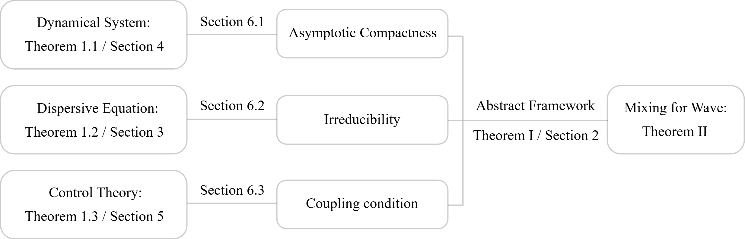
As stated in Section 1.2.2, the proof of Theorem B is based on several intermediate results for the deterministic equation (1.8). In what follows, we shall provide brief statements of these results, i.e. Theorems 1.1-1.3 below, and describe their relations to the randomly forced equation (1.3). See Figure 2 for a rough picture of the proof.

1.3.1. Asymptotic compactness

In order to verify hypothesis (𝐇)(\mathbf{H}), the initial step is to construct a compact subset of \mathcal{H}, which is exponentially attracting for (1.8). In the construction, one thing to be careful is that the regularity of attracting set should be high enough to carry the irreducibility and coupling construction. Accordingly, we shall prove the existence of an 4/7\mathcal{H}^{\scriptscriptstyle 4/7}-bounded attracting set for (1.8). In the language of dynamical system, such property can be described as

(,4/7)(\mathcal{H},\mathcal{H}^{\scriptscriptstyle 4/7})-asymptotic compactness”.

The proof of this result constitutes the main content of Section 4.

Theorem 1.1 (Asymptotic compactness).

Assume that a(x)a(x) satisfies (1.5). Then for every R0>0R_{0}>0, there exists a bounded subset 4/7\mathscr{B}_{\scriptscriptstyle 4/7} of 4/7\mathcal{H}^{\scriptscriptstyle 4/7} and constants C,κ>0C,\kappa>0 such that if

the force fbelongs to B¯L(+;H4/7)(R0),\text{the force }f\ \text{belongs to }\overline{B}_{L^{\infty}(\mathbb{R}^{+};H^{\scriptscriptstyle 4/7})}(R_{0}),

then the solution uu of (1.8) satisfies that

dist(u[t],4/7)C(1+Eu(0))eκt,t0,{\rm dist}_{\mathcal{H}}(u[t],\mathscr{B}_{\scriptscriptstyle 4/7})\leq C\left(1+E_{u}(0)\right)e^{-\kappa t},\quad\forall\,t\geq 0,

where dist(,){\rm dist}_{\mathcal{H}}(\cdot,\cdot) denotes the Hausdorff pseudo-distance in \mathcal{H} (see (2.1) later).

A more general version of Theorem 1.1, as well as the asymptotic compactness in a “physical” space 1\mathcal{H}^{1}, is contained in Theorem 4.1. By taking R0R_{0} sufficiently large so that ηB¯L(+;H4/7)(R0)\eta\in\overline{B}_{L^{\infty}(\mathbb{R}^{+};H^{\scriptscriptstyle 4/7})}(R_{0}) almost surely (see Remark 1.3), one can check that the attraction of 4/7\mathscr{B}_{\scriptscriptstyle 4/7} also works on the solution paths of (1.3). Hence, the hypothesis of asymptotic compactness in (𝐇)(\mathbf{H}) is verified with 𝒴=4/7¯\mathcal{Y}=\overline{\mathscr{B}_{\scriptscriptstyle 4/7}}; see Section 6.1 for more details.

When a(x)a0>0a(x)\equiv a_{0}>0, the conclusion of Theorem 1.1 is rather standard; see, e.g., [110]. On the other hand, the case of localized damping is much more subtle, which is up to now understood only in the autonomous setting, i.e.

f(t,x)f(x).f(t,x)\equiv f(x).

To address the localized damping, one of the approaches is provided in [48] and consists mainly of the following properties:

  • The unique continuation for a homogeneous equation in the form

    v+p(t,x)v=0,t[0,T],\boxempty v+p(t,x)v=0,\quad t\in[0,T], (1.12)

    obtained by linearizing the equation considered there and removing the damping term555The unique continuation says that if a solution of (1.12) vanishes on the effective domain of damping, then it vanishes on the entire domain; see, e.g., [96]..

  • The monotonicity of the energy, which can be readily derived in the autonomous setting.

The combination of them enables one to deduce the global dissipativity (i.e. the existence of an absorbing set) for the equation. As a consequence, the asymptotic compactness (and hence the existence of global attractor) follows in a fairly standard way.

Another approach is to invoke the unique continuation just mentioned for deriving the gradient structure [64] for the corresponding dynamical system. This implies the asymptotic compactness without any explicit discussion of dissipativity. See, e.g., [25, 66] for the related literature.

Does the asymptotic compactness hold for (1.8) with a nonzero force f(t,x)f(t,x) depending on tt? This problem remains open mainly due to the following difficulties:

  • (1)(1)

    The damping coefficient a(x)a(x) can be localized in the physical space (see Remark 1.2).

  • (2)(2)

    In the presence of f(t,x)f(t,x) the linearized problem of (1.8) is inhomogeneous, and the unique continuation does not make sense in such situation. As an aftermath, the discussion of gradient structure becomes much more complicated.

  • (3)(3)

    The energy function for (1.8) is not necessarily non-increasing in time, which can be seen from the flux estimate

    Eu(T)Eu(0)=DT[a(x)|tu|2+ftu],T0.E_{u}(T)-E_{u}(0)=\int_{D_{T}}\left[-a(x)|\partial_{t}u|^{2}+f\partial_{t}u\right],\quad\forall\,T\geq 0. (1.13)

The main task of Section 4 later is to give an affirmative answer to this question, and then the conclusion as in Theorem 1.1 is obtained.

The ideas and methods proposed for overcoming these obstacles contribute to part of novelty of the present paper. Roughly speaking, we observe that when the energy of a solution is large, it is non-increasing in discrete times (see Lemma 4.2): there exist constants T0,A0>0T_{0},A_{0}>0 such that

Eu(0)A0Eu(T0)Eu(0).E_{u}(0)\geq A_{0}\quad\Rightarrow\quad E_{u}(T_{0})\leq E_{u}(0). (1.14)

In comparison, it is non-increasing in continuous time when f(t,x)0f(t,x)\equiv 0. Property (1.14) will be obtained by establishing

0TEu(t)𝑑t\displaystyle\int_{0}^{T}E_{u}(t)dt Eu(T)+DT[a(x)|tu|2+u2+|ftu|+|f|2],\displaystyle\lesssim E_{u}(T)+\int_{D_{T}}\left[a(x)|\partial_{t}u|^{2}+u^{2}+|f\partial_{t}u|+|f|^{2}\right],

by means of the multiplier technique, where the related constant is uniform for T,u,fT,u,f. The preceding estimate extracts more information from the flux (in comparison with (1.13)), illustrating roughly the propagation of localized dissipation to the whole system.

In the sequel, it will be demonstrated that such type of “discrete monotonicity” is sufficient for the global dissipativity of (1.8). Based on the dissipativity, we arrive at the (,4/7)(\mathcal{H},\mathcal{H}^{\scriptscriptstyle 4/7})-asymptotic compactness (in the absence of gradient structure), as desired, by using some estimations on the basis of Strichartz estimates (see [10, 20] and also Proposition 3.2 later).

1.3.2. Irreducibility

As mentioned in Section 1.2, we verify the irreducibility hypothesis in (𝐇)(\mathbf{H}), by invoking the global stability of an equilibrium for the unforced problem, i.e. (1.8) with f(t,x)0f(t,x)\equiv 0. To this end, we shall use the following result due to Zuazua [113].

Theorem 1.2 (Exponential decay; [113]).

Assume that a(x)a(x) satisfies (1.5). Then there exist constants C,γ>0C,\gamma>0 such that

Eu(t)CeγtEu(0),t0E_{u}(t)\leq Ce^{-\gamma t}E_{u}(0),\quad\forall\,t\geq 0 (1.15)

for any global solution uu of (1.8) with f(t,x)0f(t,x)\equiv 0.

See Proposition 3.4 for a direct consequence of Theorem 1.2, describing the global stability of zero equilibrium. This, combined with setting (𝐒𝟐)(\mathbf{S2}), could give rise to the irreducibility for (1.3); see Section 6.2 for more details. Let us mention that the approach of type “irreducibility via global stability” has been widely used both in the cases of white noise [59, 51] and bounded noise [72, 100].

The stability of the damped wave equations is an active research topic in the recent decades; see, e.g., [66, 36, 70, 29, 68, 67, 97]. In the context of Γ\Gamma-type geometric condition (involved in setting (𝐒𝟏)(\mathbf{S1})), the global stability of type (1.15) has been fully studied for wave equations with defocusing nonlinearities, which is based on the multiplier technique developed in [85]. Another approach to the global stability is within the framework of the microlocal analysis (see, e.g., [19]), where the so-called geometric control condition (GCC for abbreviation) is introduced [5], and which gives almost sharp stability results.

In particular, we mention here that the GCC-based result in [66] is also sufficient for verifying the irreducibility hypothesis, although it is of local type, i.e., the constants C,γC,\gamma in (1.15) depends on the size of initial data. This is mainly because the irreducibility involved in our criterion is required to work only on a compact set. Therefore, there seems to be some hope in extending the result of Theorem B to the setting of GCC; the key step would be to establish the asymptotic compactness as in Theorem 1.1 for such case.

1.3.3. Coupling condition

Inspired by the idea of “controllability implies mixing” developed in [100, 102], the verification of coupling hypothesis will be based on a squeezing property for the associated controlled system:

{u+a(x)tu+u3=h(t,x)+χ𝒫NTζ(t,x),xD,u[0]=(u0,u1)=u0.\begin{cases}\boxempty u+a(x)\partial_{t}u+u^{3}=h(t,x)+\chi\mathscr{P}^{\scriptscriptstyle T}_{\scriptscriptstyle N}\zeta(t,x),\quad x\in D,\\ u[0]=(u_{0},u_{1})=u^{0}.\end{cases} (1.16)

Here, h(t,x)h(t,x) is a given external force, ζ(t,x)\zeta(t,x) stands for the control, and 𝒫NT\mathscr{P}^{\scriptscriptstyle T}_{\scriptscriptstyle N} denotes the projection from L2(DT)L^{2}(D_{T}) to the finite-dimensional space

span{ejαkT,1j,kN}.\text{span}\{e_{j}\alpha^{\scriptscriptstyle T}_{k},1\leq j,k\leq N\}.

We refer the reader to the monograph [26] by Coron for comprehensive descriptions of the italic terminology below from the control theory. Our analysis for the control problem is placed in Section 5.

The squeezing property for (1.16) is collected in the following.

Theorem 1.3 (Squeezing property).

Assume that a(x),χ(x)a(x),\,\chi(x) satisfy setting (𝐒𝟏)(\mathbf{S1}). Then for every T>𝐓T>\mathbf{T} and R1,R2>0R_{1},R_{2}>0, there exist constants N+N\in\mathbb{N}^{+} and d>0d>0 such that for every u0,u^0B¯4/7(R1)u^{0},\hat{u}^{0}\in\overline{B}_{\mathcal{H}^{\scriptscriptstyle 4/7}}(R_{1}) with

u0u^0d\|u^{0}-\hat{u}^{0}\|_{{}_{\mathcal{H}}}\leq d

and hB¯L2(0,T;H4/7)(R2)h\in\overline{B}_{L^{2}(0,T;H^{\scriptscriptstyle 4/7})}(R_{2}), there is a control ζL2(DT)\zeta\in L^{2}(D_{T}) satisfying

S(u^0,h)S(u0,h+χ𝒫NTζ)14u^0u0,\|S(\hat{u}^{0},h)-S(u^{0},h+\chi\mathscr{P}^{\scriptscriptstyle T}_{\scriptscriptstyle N}\zeta)\|_{{}_{\mathcal{H}}}\leq\frac{1}{4}\|\hat{u}^{0}-u^{0}\|_{{}_{\mathcal{H}}}, (1.17)

where SS is defined by (1.9).

See Theorem 5.1 for a stronger statement of Theorem 1.3, where more information on the structure of control, also necessary in dealing with (1.3), is involved. Denote by \ell the common law of ηn\eta_{n} in L2(DT)L^{2}(D_{T}), and by \mathcal{E} its support. The parameters R1,R2R_{1},R_{2} can be appropriately chosen so that

𝒴B¯4/7(R1),B¯L2(0,T;H4/7)(R2).\mathcal{Y}_{\infty}\subset\overline{B}_{\mathcal{H}^{\scriptscriptstyle 4/7}}(R_{1}),\quad\mathcal{E}\subset\overline{B}_{L^{2}(0,T;H^{\scriptscriptstyle 4/7})}(R_{2}).

Then, combined with two classical results for optimal couplings and an estimate for the total variation distance (see Appendix A), the squeezing (1.17) would imply the coupling condition for (1.3); see Section 6.3 for more details.

Control problems, including controllability and stabilization666 In control theory, the controllability means that for any given two states in the phase space, there is a control force driving the system from one state to the other in a finite time. On the other hand, the stabilization problem is whether or not a controlled system can be asymptotically stabilized to a (non-)stationary solution. See [26] for more information., for nonlinear wave equations (and other dispersive equations) with localized control have attracted much attention in the last few decades; see, e.g., [35, 14, 13, 34, 29, 83, 4, 1]. In particular, the literature with low-frequency controls in general concentrates on the stabilization problem, as the controllability properties are usually valid just for the low frequency in the evolution. Such subtlety can be partly explained by a viewpoint of Dehman and Lebeau [35] that “the energy of each scale of the control force depends (almost) only on the energy of the same scale in the states that one wants to control”.

Since the squeezing property considered here is closely related to the stabilization (see Remark 5.5), the strategy of our proof for Theorem 1.3 is inspired by the ideas coming from the theories of stabilization, in particular, the prior works [108, 109, 1, 71], with technical modifications adapted to (1.16). The methodology we introduce for proving Theorem 1.3 is “frequency analysis”, i.e.,

duality argumentobservability inequality damping effect low-frequency controllability high-frequency dissipation squeezing

Below we give a discussion of the main novelty of our approach, and refer to Section 5.1 later for a technical outline of proof for Theorem 1.3.

  • (1)(1)

    We establish a new version of duality between controllability and observability in the context of (1.16), i.e. Proposition 5.2, which not only translates the low-frequency controllability problem to the verification of observability inequality

    0T𝒫NT(χφ)(t)Hs2φ[T]1s2with some s(0,1)\int_{0}^{T}\|\mathscr{P}^{\scriptscriptstyle T}_{\scriptscriptstyle N}(\chi\varphi)(t)\|^{2}_{{}_{H^{\scriptscriptstyle-s}}}\gtrsim\|\varphi[T]\|^{2}_{{}_{\mathcal{H}^{\scriptscriptstyle-1-s}}}\quad\text{with some }s\in(0,1)

    for solutions φ\varphi of the adjoint system, but also helps us to improve the regularity of control. The latter plays an important role in deriving the strong dissipation for the high-frequency system. As a by-product, the quantitative controllability can be obtained within our framework and the control is expressed in an explicit form.

  • (2)(2)

    The presence of space-dependent coefficient a(x)a(x) leads to various technical complications (see Remark 1.2), so that the arguments used for observability inequality in the prior works, e.g., [1, 111, 47, 35], may not be easily applicable in the context involved here. Part of our analyses aim at dealing with such issue, involving unique continuation, Carleman estimates and Hilbert uniqueness method (HUM for abbreviation). As a consequence, the proof of observability constitutes a delicate part of our control analysis.

1.4. Organization of the present paper

In Section 2, we present a rigorous statement of our criterion (i.e., Theorem A) and its proof. In the sequel, the intermediate results mentioned in Section 1.3 are precisely provided in Sections 3-5.

We in Section 3 give a complete statement of global stability result for the unforced version of (1.8), i.e., Theorem 1.2, as well as some energy and dispersive estimates that will be useful in later sections. The main content of Section 4 is to prove a stronger version of Theorem 1.1, the asymptotic compactness for (1.8). The result therein is obtained by improving the classical arguments in global attractor for dynamical systems and by introducing the notion of discrete monotonicity. We next turn attention to the full statement and proof of squeezing property, i.e., Theorem 1.3, in Section 5. In this part, the ideas and methods in control theory will come into play.

Finally, putting the above results all together, we conclude in Section 6 with a rigorous version of Theorem B, illustrating how our criterion of exponential mixing is applied to the random wave equation (1.3).

Appendixes A and B collect some auxiliary results and proofs that are needed in our probabilistic and control analyses of the main text, respectively. In addition, an index of symbols is contained in Appendix C.

Note. From now on, the letter CC denotes the generic constant which may change from line to line.

2. Mixing criterion for random dynamical systems

The primary objective of this section is to establish our asymptotic-compactness-based criterion, i.e. Theorem 2.1 below, as briefly stated in Theorem A. It serves as a fundamental instrument to demonstrate exponential mixing for model (1.3) in Section 6.

We begin with some necessary notations and conventions. Let 𝒳\mathcal{X} and 𝒵\mathcal{Z} be Polish spaces, and the metric on 𝒳\mathcal{X} is denoted by dd. We write B𝒳(x,r)={y𝒳;d(x,y)<r}B_{\mathcal{X}}(x,r)=\{y\in\mathcal{X};d(x,y)<r\} for x𝒳x\in\mathcal{X} and r>0r>0, and B𝒳(r)=B𝒳(0,r)B_{\mathcal{X}}(r)=B_{\mathcal{X}}(0,r) when 𝒳\mathcal{X} is a separable Banach space. Let us denote B¯𝒳(r)=B𝒳(r)¯\overline{B}_{\mathcal{X}}(r)=\overline{B_{\mathcal{X}}(r)}. Define

dist𝒳(x,A)=infyAd(x,y),x𝒳,A𝒳.\text{dist}_{\mathcal{X}}(x,A)=\inf_{y\in A}d(x,y),\quad x\in\mathcal{X},\,A\subset\mathcal{X}. (2.1)

If there is no danger of confusion, we shall omit the subscript 𝒳\mathcal{X} of the above notations for the sake of simplicity. In addition, let us lay out some collections related to 𝒳\mathcal{X}: (𝒳)\mathcal{B}(\mathcal{X}) denotes its Borel σ\sigma-algebra; 𝒫(𝒳)\mathcal{P}(\mathcal{X}) is the set of Borel probability measures on 𝒳\mathcal{X}; by Bb(𝒳)B_{b}(\mathcal{X}), Cb(𝒳)C_{b}(\mathcal{X}) we denote the set of bounded Borel/continuous functions on 𝒳\mathcal{X}, endowed with the supremum norm \|\cdot\|_{\infty}, respectively; Lb(𝒳)L_{b}(\mathcal{X}) stands for the set of bounded Lipschitz functions. For fLb(𝒳)f\in L_{b}(\mathcal{X}), we denote its Lipschitz norm by

fL:=f+supxy|f(x)f(y)|d(x,y).\|f\|_{L}:=\|f\|_{\infty}+\sup_{x\neq y}\frac{|f(x)-f(y)|}{d(x,y)}.

For fBb(𝒳)f\in B_{b}(\mathcal{X}) and μ𝒫(𝒳)\mu\in\mathcal{P}(\mathcal{X}), we write f,μ=𝒳f(x)μ(dx)\langle f,\mu\rangle=\int_{\mathcal{X}}f(x)\mu(dx). The dual-Lipschitz distance in 𝒫(𝒳)\mathcal{P}(\mathcal{X}) is defined as

μνL=supfLb(𝒳),fL1|f,μf,ν|,μ,ν𝒫(𝒳),\|\mu-\nu\|_{L}^{*}=\sup_{f\in L_{b}(\mathcal{X}),\|f\|_{L}\leq 1}|\langle f,\mu\rangle-\langle f,\nu\rangle|,\quad\mu,\nu\in\mathcal{P}(\mathcal{X}),

which metricizes the weak topology; see, e.g., [78, Section 1.2.3].

Recall that for μ1,μ2𝒫(𝒳)\mu_{1},\mu_{2}\in\mathcal{P}(\mathcal{X}), a pair of 𝒳\mathcal{X}-valued random variables (ξ1,ξ2)(\xi_{1},\xi_{2}) is called a coupling for μ1\mu_{1} and μ2\mu_{2}, if 𝒟(ξi)=μi\mathscr{D}(\xi_{i})=\mu_{i}, i=1,2i=1,2. We denote by 𝒞(μ1,μ2)\mathscr{C}(\mu_{1},\mu_{2}) the set of these couplings.

The general settings of random dynamical systems and the main theorems are presented in Section 2.1, followed by a brief outline of the proof. The detailed proof is collected in Section 2.2.

2.1. Settings and general results

Let us recall that the considered Markov process {xn;n}\{x_{n};n\in\mathbb{N}\} is given by (1.1),(1.2), where S:𝒳×𝒵𝒳S\colon\mathcal{X}\times\mathcal{Z}\rightarrow\mathcal{X} is a locally Lipschitz mapping, and {ξn;n}\{\xi_{n};n\in\mathbb{N}\} is a sequence of 𝒵\mathcal{Z}-valued i.i.d. random variables. The common law of ξn\xi_{n} is \ell, whose support is denoted by \mathcal{E}. In order to indicate the initial condition and the random inputs, we also write

xn=Sn(x;ξ0,,ξn1)=Sn(x;𝝃),n+x_{n}=S_{n}(x;\xi_{0},\cdots,\xi_{n-1})=S_{n}(x;\bm{\xi}),\quad n\in\mathbb{N}^{+} (2.2)

with 𝝃:={ξn;n}\bm{\xi}:=\{\xi_{n};n\in\mathbb{N}\}. Moreover, given a sequence 𝜻={ζn;n}𝒵\bm{\zeta}=\{\zeta_{n};n\in\mathbb{N}\}\in\mathcal{Z}^{\mathbb{N}}, we denote by

Sn(x;ζ0,,ζn1)=Sn(x;𝜻)S_{n}(x;\zeta_{0},\cdots,\zeta_{n-1})=S_{n}(x;\bm{\zeta})

the corresponding deterministic process defined by (1.1),(1.2) by replacing ξn\xi_{n} with ζn\zeta_{n}.

With the above setting, system (1.1),(1.2) defines a Feller family of discrete-time Markov processes in 𝒳\mathcal{X}; see, e.g., [78, Section 1.3]. We denote by {x;x𝒳}\{\mathbb{P}_{x};x\in\mathcal{X}\} the corresponding Markov family, by 𝔼x\mathbb{E}_{x} the corresponding expected values, and by {Pn(x,A);x𝒳,A(𝒳),n}\{P_{n}(x,A);x\in\mathcal{X},A\in\mathcal{B}(\mathcal{X}),n\in\mathbb{N}\} the corresponding Markov transition functions, i.e.,

Pn(x,A)=x(xnA).P_{n}(x,A)=\mathbb{P}_{x}(x_{n}\in A).

We use the standard notation for the corresponding Markov semigroup Pn:Bb(𝒳)Bb(𝒳)P_{n}\colon B_{b}(\mathcal{X})\rightarrow B_{b}(\mathcal{X}) and its dual Pn:𝒫(𝒳)𝒫(𝒳)P^{*}_{n}\colon\mathcal{P}(\mathcal{X})\rightarrow\mathcal{P}(\mathcal{X}) defined by

Pnf(x)=𝒳f(y)Pn(x,dy),Pnμ(A)=𝒳Pn(x,A)μ(dx)P_{n}f(x)=\int_{\mathcal{X}}f(y)P_{n}(x,dy),\quad\quad P_{n}^{*}\mu(A)=\int_{\mathcal{X}}P_{n}(x,A)\mu(dx)

for fBb(𝒳)f\in B_{b}(\mathcal{X}), μ𝒫(𝒳)\mu\in\mathcal{P}(\mathcal{X}), x𝒳x\in\mathcal{X} and A(𝒳)A\in\mathcal{B}(\mathcal{X}). Recall that a probability measure μ𝒫(𝒳)\mu\in\mathcal{P}(\mathcal{X}) is called invariant for {Pn;n}\{P_{n}^{*};n\in\mathbb{N}\} if Pnμ=μP_{n}^{*}\mu=\mu for any nn\in\mathbb{N}. Our goal is to investigate exponential mixing for the Markov process {xn;n}\{x_{n};n\in\mathbb{N}\}.

The following notion of attainable set will be used.

Definition 2.1.

For every subset 𝒴\mathcal{Y} of 𝒳\mathcal{X}, the attainable set 𝒴n\mathcal{Y}_{n} in time nn is of the form

𝒴0=𝒴,𝒴n={Sn(x,ζ0,,ζn1);x𝒴,ζ0,,ζn1},n+,\mathcal{Y}_{0}=\mathcal{Y},\quad\mathcal{Y}_{n}=\{S_{n}(x,\zeta_{0},\cdots,\zeta_{n-1});x\in\mathcal{Y},\zeta_{0},\cdots,\zeta_{n-1}\in\mathcal{E}\},\quad n\in\mathbb{N}^{+},

and the attainable set 𝒴\mathcal{Y}_{\infty} is given by

𝒴=n𝒴n¯.\mathcal{Y}_{\infty}=\overline{\bigcup_{n\in\mathbb{N}}\mathcal{Y}_{n}}.

With the preparations above at hand, we list the hypotheses involved in our general criterion:

  • (𝐀𝐂\mathbf{AC})

    (Asymptotic compactness) There exists a compact subset 𝒴\mathcal{Y} of 𝒳\mathcal{X}, a constant κ>0\kappa>0, and a measurable function V:𝒳+V\colon\mathcal{X}\rightarrow\mathbb{R}^{+} which is bounded on bounded sets, such that

    dist(Sn(x;𝜻),𝒴)V(x)eκn\text{dist}(S_{n}(x;\bm{\zeta}),\mathcal{Y})\leq V(x)e^{-\kappa n} (2.3)

    for any x𝒳,𝜻x\in\mathcal{X},\,\bm{\zeta}\in\mathcal{E}^{\mathbb{N}} and n+n\in\mathbb{N}^{+}.

Our observation on the asymptotic compactness has been described in Section 1.1. In particular, using the compactness of both 𝒴\mathcal{Y} and \mathcal{E}, straightforward compactness arguments imply that the attainable set 𝒴\mathcal{Y}_{\infty} is compact in 𝒳\mathcal{X}; see Proposition 2.2 later.

  • (𝐈\mathbf{I})

    (Irreducibility on compact set) There exists a point z𝒴z\in\mathcal{Y} such that for every ε>0\varepsilon>0, one can find an integer m=m(ε)+m=m(\varepsilon)\in\mathbb{N}^{+} satisfying

    infx𝒴Pm(x,B(z,ε))>0.\inf_{x\in\mathcal{Y}_{\infty}}P_{m}(x,B(z,\varepsilon))>0. (2.4)
  • (𝐂\mathbf{C})

    (Coupling condition on compact set) There exists a constant r[0,1)r\in[0,1) such that for every x,x𝒴x,x^{\prime}\in\mathcal{Y}_{\infty}, there is ((x,x),(x,x))𝒞(P1(x,),P1(x,))(\mathcal{R}(x,x^{\prime}),\mathcal{R}^{\prime}(x,x^{\prime}))\in\mathscr{C}(P_{1}(x,\cdot),P_{1}(x^{\prime},\cdot)) on a same probability space (Ω,,)(\Omega,\mathcal{F},\mathbb{P}), satisfying

    (d((x,x),(x,x))>rd(x,x))g(d(x,x)),\mathbb{P}(d(\mathcal{R}(x,x^{\prime}),\mathcal{R}^{\prime}(x,x^{\prime}))>rd(x,x^{\prime}))\leq g(d(x,x^{\prime})), (2.5)

    where g:++g\colon\mathbb{R}^{+}\rightarrow\mathbb{R}^{+} is a continuous increasing function with

    g(0)=0,lim supn1nlng(rn)<0,g(0)=0,\quad\limsup\limits_{n\rightarrow\infty}\frac{1}{n}\ln g(r^{n})<0, (2.6)

    and the mappings ,:𝒴×𝒴×Ω𝒳\mathcal{R},\mathcal{R}^{\prime}\colon\mathcal{Y}_{\infty}\times\mathcal{Y}_{\infty}\times\Omega\rightarrow\mathcal{X} are measurable.

The last two hypotheses originate from the previous frameworks of ergodicity and mixing. More precisely, the irreducibility indicates that a common state can be reached by the dynamics regardless of the initial conditions, previously used to derive the unique ergodicity (see, e.g., [61, 42, 78]). On the other hand, the coupling condition can be understood as a one-step smoothing effect of the Markov process analogous to the asymptotic strong Feller property (but only for regular solutions). It is directly motivated by the work of [100], and can be also traced to the earlier literature [76, 58, 91, 90].

As a more precise version of Theorem A, what follows is one of the main results of this paper, providing a criterion of exponential mixing. Its proof is contained in Section 2.2.

Theorem 2.1.

Assume that the support \mathcal{E} of \ell is compact in 𝒵\mathcal{Z}, and hypotheses (𝐀𝐂)(\mathbf{AC}), (𝐈)(\mathbf{I}) and (𝐂)(\mathbf{C}) are satisfied. Then the Markov process {xn;n}\{x_{n};n\in\mathbb{N}\} has a unique invariant measure μ𝒫(𝒳)\mu_{*}\in\mathcal{P}(\mathcal{X}) with compact support. Moreover, there exist constants C,β>0C,\beta>0 such that

PnνμLCeβn(1+𝒳V(x)ν(dx))\|P_{n}^{*}\nu-\mu_{*}\|_{L}^{*}\leq Ce^{-\beta n}\left(1+\int_{\mathcal{X}}V(x)\nu(dx)\right) (2.7)

for any ν𝒫(𝒳)\nu\in\mathcal{P}(\mathcal{X}) such that 𝒳V(x)ν(dx)<\int_{\mathcal{X}}V(x)\nu(dx)<\infty and nn\in\mathbb{N}.

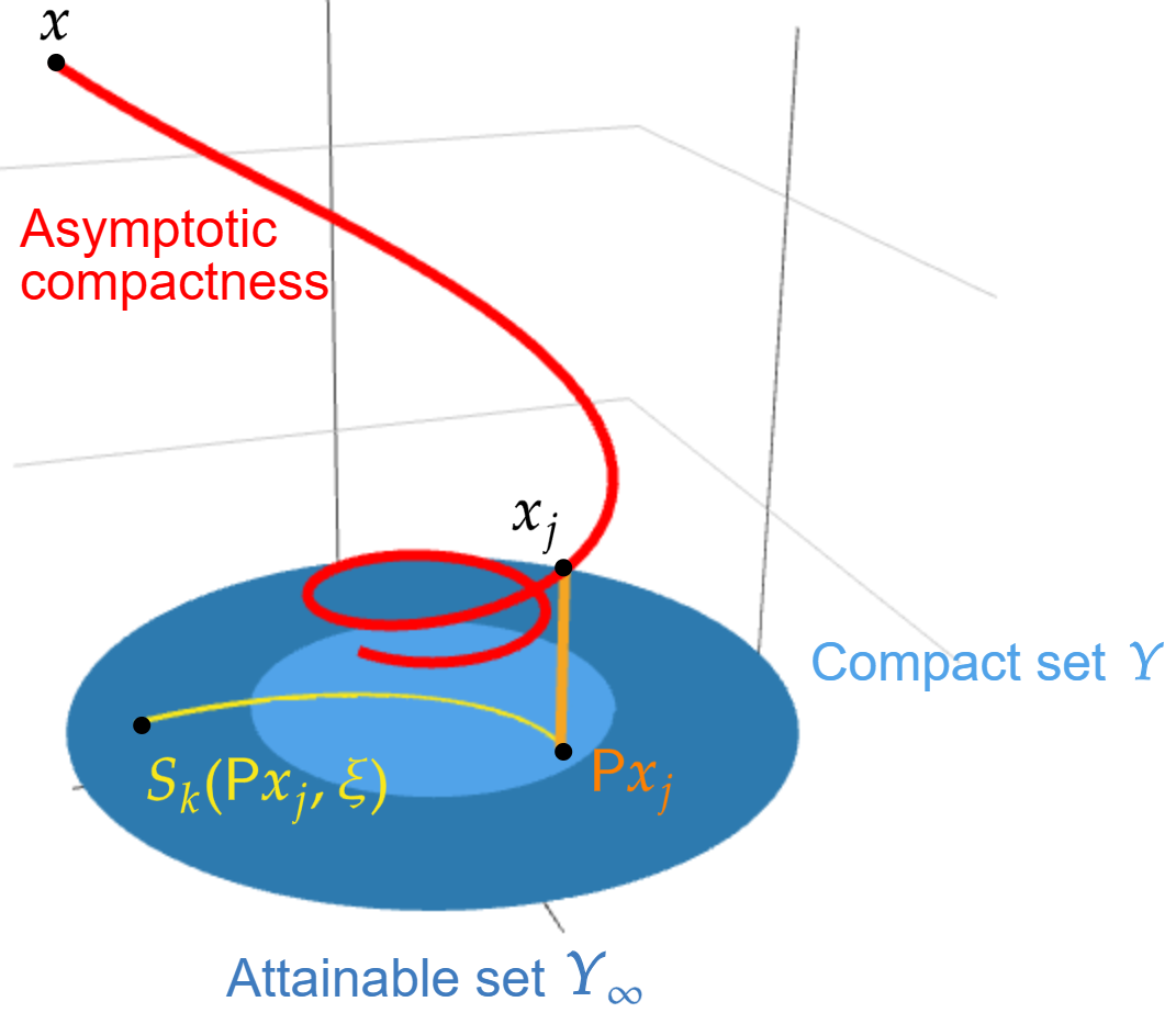
Outline of proof for Theorem 2.1. We now present a brief overview of the proof for our result, highlighting its main contribution. Our strategy is to first establish mixing on the regular subspace 𝒴\mathcal{Y}_{\infty}, and then extend to the entire space; see Figure 3 for a rough picture777This picture is just for illustration, but not rigorous, since neither the attracting set 𝒴\mathcal{Y} nor the attainable set 𝒴\mathcal{Y}_{\infty} can be in a hyperplane in general.. The proof is divided into three steps:

Step 1 (Existence of an invariant compactum). We begin by demonstrating that the natural working space 𝒴\mathcal{Y}_{\infty} is compact and invariant due to hypothesis (AC); see Proposition 2.2. This allows a coupling construction to deduce the exponential mixing on 𝒴\mathcal{Y}_{\infty} in the next step.

Step 2 (Mixing on the invariant compactum). In order to establish the mixing on 𝒴\mathcal{Y}_{\infty}, we shall invoke Kuksin–Shirikyan’s framework (see [78, 99]), under the hypotheses (𝐈)(\mathbf{I}) and (𝐂)(\mathbf{C}). More precisely, let us consider a Markov process {𝒙n;n}\{\vec{\bm{x}}_{n};n\in\mathbb{N}\} on the product space 𝒴×𝒴\mathcal{Y}_{\infty}\times\mathcal{Y}_{\infty} with marginals Pn(x,)P_{n}(x,\cdot) and Pn(x,)P_{n}(x^{\prime},\cdot), where x,x𝒴x,x^{\prime}\in\mathcal{Y}_{\infty}. The process {𝒙n;n}\{\vec{\bm{x}}_{n};n\in\mathbb{N}\} is called an extension of the process {xn;n}\{x_{n};n\in\mathbb{N}\}, as detailed in Appendix A.1.1. Hypothesis (I) guarantees a recurrence property: the two components of 𝒙n\vec{\bm{x}}_{n} can be made to approach each other with arbitrary proximity within a finite time almost surely. Once the two components of 𝒙n\vec{\bm{x}}_{n} have become sufficiently close, the coupling condition (C) ensures that they will continue to converge with a positive probability; such convergence is referred to as squeezing. Consequently, the Markov property and this loop collectively indicate exponential mixing on 𝒴\mathcal{Y}_{\infty}. For further details, please refer to Proposition 2.3.

Step 3 (Extending mixing to the original space). The last step is to extend the 𝒴\mathcal{Y}_{\infty}-restricted mixing to the entire state space. This is established via the exponential attraction of the invariant compactum 𝒴\mathcal{Y}_{\infty} (guaranteed by hypothesis (AC)) together with a projection procedure; see Proposition 2.4.

Refer to caption
Figure 3. Outline of proof for Theorem 2.1.

As straightforward applications of Theorem 2.1, we have the following limit theorems, including the strong law of large numbers and central limit theorem for bounded Lipschitz observables. The proofs are based on standard martingale decomposition procedures and are placed in Appendix A.4.

Proposition 2.1.

Under the assumptions of Theorem 2.1, the following assertions hold:

  • (1)(1)

    (Strong law of large numbers) For every fLb(𝒳)f\in L_{b}(\mathcal{X}) and x𝒳x\in\mathcal{X},

    limn1nk=0n1f(xk)=f,μalmost surely.\lim\limits_{n\rightarrow\infty}\frac{1}{n}\sum_{k=0}^{n-1}f(x_{k})=\langle f,\mu_{*}\rangle\quad\text{almost surely}.
  • (2)(2)

    (Central limit theorem) For every fLb(𝒳)f\in L_{b}(\mathcal{X}), there exists a constant σf0\sigma_{f}\geq 0 such that

    1nk=0n1(f(xk)f,μ)𝒩(0,σf2) as n\frac{1}{\sqrt{n}}\sum_{k=0}^{n-1}(f(x_{k})-\langle f,\mu_{*}\rangle)\rightarrow\mathcal{N}(0,\sigma_{f}^{2})\quad\text{ as }n\rightarrow\infty

    for any x𝒳x\in\mathcal{X}, where 𝒩(0,σf2)\mathcal{N}(0,\sigma_{f}^{2}) denotes a normal random variable with zero mean and variance σf2\sigma_{f}^{2}, and the convergence is in the sense of distribution.

2.2. Proof of exponential mixing

As previously mentioned, the proof of Theorem 2.1 consists of three steps.

2.2.1. Existence of an invariant compactum.

As mentioned in Step 1 of Section 2.1, a straightforward consequence of hypothesis (𝐀𝐂)(\mathbf{AC}) is that 𝒴\mathcal{Y}_{\infty} is a compact invariant set. Using (2.8) and the Feller property, a standard Kryloy–Bogolyubov averaging procedure yields that the Markov process {xn;n}\{x_{n};n\in\mathbb{N}\} admits an invariant measure.

Proposition 2.2.

Assume that hypothesis (𝐀𝐂)(\mathbf{AC}) holds and \mathcal{E} is compact in 𝒵\mathcal{Z}. Then 𝒴\mathcal{Y}_{\infty} is compact in 𝒳\mathcal{X} and invariant under SS in the sense that

S(𝒴×)𝒴.S(\mathcal{Y}_{\infty}\times\mathcal{E})\subset\mathcal{Y}_{\infty}. (2.8)
Proof.

We begin by demonstrating that the set 𝒴\mathcal{Y}_{\infty} is compact. It can be observed that each set 𝒴n\mathcal{Y}_{n} is compact, given that both 𝒴\mathcal{Y} and \mathcal{E} are compact. Let us now consider a sequence {yn;n}\{y^{n};n\in\mathbb{N}\} contained in l𝒴l\bigcup_{l\in\mathbb{N}}\mathcal{Y}_{l}. Then, there exists lnl_{n}\in\mathbb{N} and xn𝒴x^{n}\in\mathcal{Y} such that either yn=xny^{n}=x^{n}, or

yn=Sln(xn;ζ0n,,ζln1n)𝒴lny^{n}=S_{l_{n}}(x^{n};\zeta_{0}^{n},\cdots,\zeta_{l_{n}-1}^{n})\in\mathcal{Y}_{l_{n}}

for some ζjn,j=0,,ln1\zeta_{j}^{n}\in\mathcal{E},\ j=0,\cdots,l_{n}-1.

If the sequence {ln;n}\{l_{n};n\in\mathbb{N}\} is bounded, then taking m=max{ln;n}m=\max\{l_{n};n\in\mathbb{N}\}, it follows that {yn;n}\{y^{n};n\in\mathbb{N}\} is contained in 0lm𝒴l\bigcup_{0\leq l\leq m}\mathcal{Y}_{l}, hence is relatively compact. In the case where {ln;n}\{l_{n};n\in\mathbb{N}\} is unbounded, assume that lnl_{n}\rightarrow\infty without loss of generality. By hypothesis (AC), it follows that

dist(yn,𝒴)V(xn)eκln0{\rm dist}(y^{n},\mathcal{Y})\leq V(x^{n})e^{-\kappa l_{n}}\rightarrow 0

as nn\rightarrow\infty. Here, we have tacitly used the boundedness of {xn;n}\{x^{n};n\in\mathbb{N}\}. Thus, by the compactness of 𝒴\mathcal{Y}, we conclude that the sequence {yn;n}\{y^{n};n\in\mathbb{N}\} is relatively compact. Consequently, the compactness of 𝒴\mathcal{Y}_{\infty} follows immediately.

It remains to prove that 𝒴\mathcal{Y}_{\infty} is invariant. In view of its compactness, this is a direct consequence of the continuity of SS. ∎

2.2.2. Mixing on the invariant compactum.

Based on Proposition 2.2, we shall establish the exponential mixing for {xn;n}\{x_{n};n\in\mathbb{N}\} acting on the invariant compactum 𝒴\mathcal{Y}_{\infty}. This is presented as the following result.

Proposition 2.3.

Under the assumptions of Theorem 2.1, the Markov process {xn;n}\{x_{n};n\in\mathbb{N}\} on 𝒴\mathcal{Y}_{\infty} admits a unique invariant measure μ𝒫(𝒴)\mu_{*}\in\mathcal{P}(\mathcal{Y}_{\infty}). Moreover, there exist constants C0,β0>0C_{0},\beta_{0}>0 such that

PnνμLC0eβ0n\|P_{n}^{*}\nu-\mu_{*}\|^{*}_{L}\leq C_{0}e^{-\beta_{0}n} (2.9)

for any ν𝒫(𝒴)\nu\in\mathcal{P}(\mathcal{Y}_{\infty}) and nn\in\mathbb{N}.

In order to demonstrate Proposition 2.3, we employ a coupling construction. In particular, we utilize Theorem A.1, which is a special case of the general result established by Kuksin and Shirikyan [78, 99]. The proof of this proposition is analogous to that presented in [102, Theorem 1.1], where the approximate controllability and local stabilisability are replaced by irreducibility and coupling condition in the present setting. For the reader’s convenience, we provide an outline of the proof below, while the details can be found in Appendix A.3.

Sketch of proof.

Following the route described in Step 2 of Section 2.1, we shall transform the problem into the verification of the recurrence and squeezing properties for an extension process, which will be appropriately constructed. The proof will be divided into three steps.

Step 2.1 (Extension construction). Let 𝒀=𝒴×𝒴\bm{Y}_{\infty}=\mathcal{Y}_{\infty}\times\mathcal{Y}_{\infty} and constant δ(0,1)\delta\in(0,1) be specified later. We introduce the diagonal set in 𝒀\bm{Y}_{\infty} by

𝓓δ={(x,x)𝒀;d(x,x)δ}.\bm{\mathcal{D}}_{\delta}=\{(x,x^{\prime})\in\bm{Y}_{\infty};d(x,x^{\prime})\leq\delta\}.

Then, define a coupling operator on 𝒀\bm{Y}_{\infty} by the relation

𝑹(x,x)={((x,x),(x,x))for (x,x)𝓓δ,(S(x,ξ),S(x,ξ))otherwise,\bm{{R}}(x,x^{\prime})=\begin{cases}(\mathcal{R}(x,x^{\prime}),\mathcal{R}^{\prime}(x,x^{\prime}))\quad&\text{for }(x,x^{\prime})\in\bm{\mathcal{D}}_{\delta},\\ (S(x,\xi),S(x^{\prime},\xi^{\prime}))&\text{otherwise},\end{cases}

where ξ\xi and ξ\xi^{\prime} are independent copies of ξ0\xi_{0}. Using this coupling operator 𝑹\bm{{R}}, we can construct a family of Markov processes {𝒙n;n}\{\vec{\bm{x}}_{n};n\in\mathbb{N}\} on 𝒀\bm{Y}_{\infty} with the following properties:

  • (1)

    {𝒙n;n}\{\vec{\bm{x}}_{n};n\in\mathbb{N}\} is an extension of {xn;n}\{x_{n};n\in\mathbb{N}\}. More precisely, the transition probability 𝑷n(𝒙,)\bm{P}_{n}(\vec{\bm{x}},\cdot) of 𝒙n\vec{\bm{x}}_{n} is a coupling of (Pn(x,),Pn(x,))(P_{n}(x,\cdot),P_{n}(x^{\prime},\cdot)) for 𝒙=(x,x)𝒀\vec{\bm{x}}=(x,x^{\prime})\in\bm{Y}_{\infty}. In what follows, we make a slight abuse of notation and write 𝒙n=(xn,xn)\vec{\bm{x}}_{n}=(x_{n},x^{\prime}_{n}).

  • (2)

    We shall show that the extension process {𝒙n;n}\{\vec{\bm{x}}_{n};n\in\mathbb{N}\} verifies the squeezing and recurrence properties on 𝓓δ\bm{\mathcal{D}}_{\delta} for some δ(0,1)\delta\in(0,1) in the following sense:
    \centerdot (Squeezing) There exist constants C1,β1>0C_{1},\beta_{1}>0 such that the random time

    𝝈:=inf{n;d(xn,xn)>rnδ}\bm{\sigma}:=\inf\{n\in\mathbb{N};d(x_{n},x_{n}^{\prime})>r^{n}\delta\}

    satisfies that

    (𝝈=)1/2,(𝝈=n)C1eβ1n\mathbb{P}(\bm{\sigma}=\infty)\geq 1/2,\quad\mathbb{P}(\bm{\sigma}=n)\leq C_{1}e^{-\beta_{1}n} (2.10)

    for any 𝒙𝓓δ\vec{\bm{x}}\in\bm{\mathcal{D}}_{\delta} and nn\in\mathbb{N}. Here, the constant r[0,1)r\in[0,1) is established by (2.5).
    \centerdot (Recurrence) There exist constants C2,β2>0C_{2},\beta_{2}>0 such that the random time

    𝝉:=inf{n;𝒙n𝓓δ}\bm{\tau}:=\inf\{n\in\mathbb{N};\vec{\bm{x}}_{n}\in\bm{\mathcal{D}}_{\delta}\}

    satisfies that

    (𝝉<)=1,(𝝉=n)C2eβ2n\mathbb{P}(\bm{\tau}<\infty)=1,\quad\mathbb{P}(\bm{\tau}=n)\leq C_{2}e^{-\beta_{2}n} (2.11)

    for any 𝒙𝒀\vec{\bm{x}}\in\bm{Y}_{\infty} and nn\in\mathbb{N}.

Once properties (1) and (2) are established, we verify the conditions of Theorem A.1, thereby completing the proof of exponential mixing on 𝒴\mathcal{Y}_{\infty}.

Step 2.2 (Verification of squeezing). In order to demonstrate the squeezing property, let us fix any 𝒙=(x,x)𝓓δ\vec{\bm{x}}=(x,x^{\prime})\in\bm{\mathcal{D}}_{\delta}. In view of the definition of 𝑹\bm{R} and the coupling hypothesis (C), it follows that

(d(x1,x1)rd(x,x))1g(d(x,x)).\mathbb{P}(d(x_{1},x^{\prime}_{1})\leq rd(x,x^{\prime}))\leq 1-g(d(x,x^{\prime})). (2.12)

This in conjunction with the Markov property allows for the application of standard iteration arguments, which in turn yield the following result:

(𝝈=)n(1g(rnd(x,x))).\displaystyle\displaystyle\mathbb{P}(\bm{\sigma}=\infty)\geq\prod_{n\in\mathbb{N}}(1-g(r^{n}d(x,x^{\prime}))).

Consequently, the first inequality in (2.10) is attained by choosing the parameter δ(0,1)\delta\in(0,1) sufficiently small and recalling that gg satisfies condition (2.6). Similarly, one can further deduce that

(𝝈=n)g(rn),\mathbb{P}(\bm{\sigma}=n)\leq g(r^{n}),

which in turn implies the second inequality in (2.10) by taking β1(0,lim supn1nlng(rn))\beta_{1}\in(0,-\limsup\limits_{n\rightarrow\infty}\tfrac{1}{n}\ln g(r^{n})).

In summary, the squeezing property follows.

Step 2.3 (Verification of recurrence). It remains to establish the recurrence (2.11). Invoking the Markov property and Borel–Cantelli lemma, it suffices to show that there exists m+m\in\mathbb{N}^{+} and p>0p>0 such that for every 𝒙𝒀\vec{\bm{x}}\in\bm{Y}_{\infty},

(𝒙m𝓓δ)p.\mathbb{P}(\vec{\bm{x}}_{m}\in\bm{\mathcal{D}}_{\delta})\geq p.

This can be achieved through the following two observations.

  • \centerdot

    The construction of the extension process allows one to verify that xnx_{n} and xnx_{n}^{\prime} are conditionally independent on the set {𝝉n}\{\bm{\tau}\geq n\}. In particular, taking hypothesis (I) into account, there exists m+m\in\mathbb{N}^{+} such that

    (𝒙m𝓓δ|𝝉m)(infx𝒴Pm(x,B(z,δ/2)))2>0\mathbb{P}(\vec{\bm{x}}_{m}\in\bm{\mathcal{D}}_{\delta}|\bm{\tau}\geq m)\geq(\inf_{x\in\mathcal{Y}_{\infty}}P_{m}(x,B(z,\delta/2)))^{2}>0
  • \centerdot

    On the other hand, let us note that 𝒙τ𝓓δ\vec{\bm{x}}_{\tau}\in\bm{\mathcal{D}}_{\delta}. Then making use of the strong Markov property and squeezing property, we get

    (𝒙m𝓓δ|𝝉<m)inf𝒙𝓓δ(𝝈=)1/2.\mathbb{P}(\vec{\bm{x}}_{m}\in\bm{\mathcal{D}}_{\delta}|\bm{\tau}<m)\geq\inf_{\vec{\bm{x}}\in\bm{\mathcal{D}}_{\delta}}\mathbb{P}(\bm{\sigma}=\infty)\geq 1/2.

In combination, these above shall imply the recurrence. The proof of Proposition 2.3 is therefore completed. ∎

Remark 2.1.

As a corollary of Proposition 2.3, it follows that supp μ𝒴\text{supp }\mu_{*}\subset\mathcal{Y}_{\infty}, which justifies the assertion that μ\mu_{*} has compact support. Indeed, by invoking hypothesis ((I)), one can further verify that supp μ\text{supp }\mu_{*} is precisely the attainable set from the singleton zz.

2.2.3. Extending mixing to the original space.

It remains to demonstrate global exponential mixing for {xn;n}\{x_{n};n\in\mathbb{N}\}, acting on the entire state space 𝒳\mathcal{X}; see Step 3 of Section 2.1. This will be done by combining the 𝒴\mathcal{Y}_{\infty}-restricted mixing described in Proposition 2.3, with the exponential attraction of the invariant compactum 𝒴\mathcal{Y}_{\infty} (due to hypothesis (AC)).

Proposition 2.4.

Under the assumptions of Theorem 2.1, the invariant measure μ\mu_{*}, established in Proposition 2.3, is globally exponential mixing in the sense of (2.7).

Proof.

To verify (2.7), it suffices to show that there exist constants C,β>0C,\beta>0 such that

|Pnf(x)f,μ|C(1+V(x))eβn|P_{n}f(x)-\langle f,\mu_{*}\rangle|\leq C(1+V(x))e^{-\beta n} (2.13)

for any fLb(𝒳)f\in L_{b}(\mathcal{X}) with fL1\|f\|_{L}\leq 1, x𝒳x\in\mathcal{X} and nn\in\mathbb{N}.

We claim that, in view of the compactness of 𝒴\mathcal{Y}, there exists a measurable map 𝖯:𝒳𝒴\mathsf{P}\colon\mathcal{X}\rightarrow\mathcal{Y} such that

d(x,𝖯x)2dist(x,𝒴)d(x,\mathsf{P}x)\leq 2\text{dist}(x,\mathcal{Y}) (2.14)

for any x𝒳x\in\mathcal{X}. Indeed, let {yn;n}\{y_{n};n\in\mathbb{N}\} be a dense sequence in 𝒴\mathcal{Y}, and

An={z𝒳;d(z,yn)<2dist(z,𝒴)}(0jn1Aj).\quad A_{n}=\left\{z\in\mathcal{X};d(z,y_{n})<2\text{dist}(z,\mathcal{Y})\right\}\setminus\left(\bigcup_{0\leq j\leq n-1}A_{j}\right).

Then one can check that 𝒳=𝒴(nAn)\mathcal{X}=\mathcal{Y}\cup(\bigcup_{n\in\mathbb{N}}A_{n}) and the sets AnA_{n}, 𝒴\mathcal{Y} are disjoint. It thus follows that the desired map 𝖯\mathsf{P} can be taken as

𝖯:𝒳𝒴,𝖯x={yn for xAn,x for x𝒴.\mathsf{P}\colon\mathcal{X}\rightarrow\mathcal{Y},\quad\mathsf{P}x=\begin{cases}y_{n}\quad&\text{ for }x\in A_{n},\\ x\quad&\text{ for }x\in\mathcal{Y}.\end{cases}

Let x𝒳x\in\mathcal{X} be arbitrarily given and recall the alternative expression (2.2) for {xn;n}\{x_{n};n\in\mathbb{N}\}. We also define the shifted sequences by 𝝃j={ξn+j;n}\bm{\xi}^{j}=\{\xi_{n+j};n\in\mathbb{N}\} for j+j\in\mathbb{N}^{+}, which is independent of xjx_{j}. With these settings, we compute that

|Pk+jf(x)f,μ|\displaystyle|P_{k+j}f(x)-\langle f,\mu_{*}\rangle| =|𝔼xf(xk+j)f,μ|\displaystyle=|\mathbb{E}_{x}f(x_{k+j})-\langle f,\mu_{*}\rangle| (2.15)
|𝔼xf(Sk(𝖯xj;𝝃j))f,μ|\displaystyle\leq|\mathbb{E}_{x}f(S_{k}(\mathsf{P}x_{j};\bm{\xi}^{j}))-\langle f,\mu_{*}\rangle|
+|𝔼x[f(Sk(xj;𝝃j))f(Sk(𝖯xj;𝝃j))]|\displaystyle\quad+|\mathbb{E}_{x}[f(S_{k}(x_{j};\bm{\xi}^{j}))-f(S_{k}(\mathsf{P}x_{j};\bm{\xi}^{j}))]|
=:I1+I2\displaystyle=:I_{1}+I_{2}

for any fLb(𝒳)f\in L_{b}(\mathcal{X}) with fL1\|f\|_{L}\leq 1 and j,kj,k\in\mathbb{N}. In the sequel, we intend to estimate each IiI_{i} separately.

From (2.9) it follows that

I1\displaystyle I_{1} =|𝔼x[𝔼xf(Sk(𝖯xj;𝝃j))f,μ|j]|\displaystyle=|\mathbb{E}_{x}[\mathbb{E}_{x}f(S_{k}(\mathsf{P}x_{j};\bm{\xi}^{j}))-\langle f,\mu_{*}\rangle|\mathcal{F}_{j}]| (2.16)
𝔼x|𝔼y(f(Sk(y;𝝃j))f,μ)|y=𝖯xj|\displaystyle\leq\mathbb{E}_{x}|\mathbb{E}_{y}(f(S_{k}(y;\bm{\xi}^{j}))-\langle f,\mu_{*}\rangle)|_{y=\mathsf{P}x_{j}}|
C0eβ0k,\displaystyle\leq C_{0}e^{-\beta_{0}k},

where n\mathcal{F}_{n} denotes the natural filtration of {xn;n}\{x_{n};n\in\mathbb{N}\}. In particular, let us mention that the RHS in (2.16) is independent of jj\in\mathbb{N}.

Thus, it suffices to get control over the size of I2I_{2}. To this end, we observe, in view of (2.3) included in hypothesis (AC), that

dist(Sn(x;𝝃),𝒴)V(x)eκn\text{dist}(S_{n}(x;\bm{\xi}),\mathcal{Y})\leq V(x)e^{-\kappa n} (2.17)

almost surely for any nn\in\mathbb{N}. On the other hand, one can derive, from the compactness of 𝒴\mathcal{Y}, that there exists a constant R>0R>0 such that

{Sn(y;𝝃);y𝒴,n}NR(𝒴):={y𝒳;dist(y,𝒴)<R},\{S_{n}(y;\bm{\xi});y\in\mathcal{Y},n\in\mathbb{N}\}\subset N_{R}(\mathcal{Y}):=\{y\in\mathcal{X};\text{dist}(y,\mathcal{Y})<R\},

almost surely. Then, taking (2.17) into account, one gets that

{xn;nK}NR(𝒴),\{x_{n};n\geq K\}\subset N_{R}(\mathcal{Y}),

almost surely, where K:=(ln(V(x)R1))/κK:=\lceil(\ln(V(x)R^{-1}))/{\kappa}\rceil. As a consequence,

Sk(xj;𝝃j),Sk(𝖯xj;𝝃j)NR(𝒴)S_{k}(x_{j};\bm{\xi}^{j}),S_{k}(\mathsf{P}x_{j};\bm{\xi}^{j})\in N_{R}(\mathcal{Y})

for any kk\in\mathbb{N} and jKj\geq K. In view of the Lipschitz continuity of SS on NR(𝒴)×N_{R}(\mathcal{Y})\times\mathcal{E}, there exists a constant L1L\geq 1 such that

I2\displaystyle I_{2} 𝔼xd(Sk(xj;𝝃j),Sk(𝖯xj;𝝃j))\displaystyle\leq\mathbb{E}_{x}d(S_{k}(x_{j};\bm{\xi}^{j}),S_{k}(\mathsf{P}x_{j};\bm{\xi}^{j})) (2.18)
Lk𝔼xd(xj,𝖯xj)\displaystyle\leq L^{k}\mathbb{E}_{x}d(x_{j},\mathsf{P}x_{j})
2V(x)Lkeκj,\displaystyle\leq 2V(x)L^{k}e^{-\kappa j},

where the last inequality follows from (2.14) and (2.17).

We are now prepared to prove (2.13). Plugging (2.16),(2.18) into (2.15), it follows that

|Pnf(x)f,μ|2V(x)Lkeκj+C0eβ0k\displaystyle|P_{n}f(x)-\langle f,\mu_{*}\rangle|\leq 2V(x)L^{k}e^{-\kappa j}+C_{0}e^{-\beta_{0}k}

for any n=k+jn=k+j with k0k\geq 0 and jKj\geq K, where we recall that fLb(𝒳)f\in L_{b}(\mathcal{X}) with fL1\|f\|_{L}\leq 1 is arbitrary. For ε(0,1)\varepsilon\in(0,1) to be specified below, we set

k=εn,j=(1ε)n,k=\lfloor\varepsilon n\rfloor,\quad j=\lceil(1-\varepsilon)n\rceil,

under which it can be derived that

|Pnf(x)f,μ|2V(x)e(κ+ε(κ+lnL))n+C0eβ0eβ0εn|P_{n}f(x)-\langle f,\mu_{*}\rangle|\leq 2V(x)e^{(-\kappa+\varepsilon(\kappa+\ln L))n}+C_{0}e^{\beta_{0}}e^{-\beta_{0}\varepsilon n}

for any n>K/(1ε)n>K/(1-\varepsilon). In conclusion, taking

{ε<κκ+lnL,β=min{κε(κ+lnL),β0ε,(1ε)κ},C=2max{C0eβ0,eβ/(1ε)Rβ/((1ε)κ)},\begin{cases}\varepsilon<\frac{\kappa}{\kappa+\ln L},\ \beta=\min\left\{\kappa-\varepsilon(\kappa+\ln L),\beta_{0}\varepsilon,(1-\varepsilon)\kappa\right\},\\ C=2\max\{C_{0}e^{\beta_{0}},e^{\beta/(1-\varepsilon)}R^{-\beta/((1-\varepsilon)\kappa)}\},\end{cases}

we have

|Pnf(x)f,μ|C(1+V(x))eβn|P_{n}f(x)-\langle f,\mu_{*}\rangle|\leq C(1+V(x))e^{-\beta n}

for any n>K/(1ε)n>K/(1-\varepsilon), while in the case of nK/(1ε)n\leq K/(1-\varepsilon),

|Pnf(x)f,μ|\displaystyle|P_{n}f(x)-\langle f,\mu_{*}\rangle| Ceβ/(1ε)Rβ/((1ε)κ)\displaystyle\leq Ce^{-\beta/(1-\varepsilon)}R^{\beta/((1-\varepsilon)\kappa)}
Ceβ/(1ε)Rβ/((1ε)κ)(1+V(x))V(x)β/((1ε)κ)\displaystyle\leq Ce^{-\beta/(1-\varepsilon)}R^{\beta/((1-\varepsilon)\kappa)}(1+V(x))V(x)^{-\beta/((1-\varepsilon)\kappa)}
C(1+V(x))eβ1ε[ln(V(x)R1)κ+1]\displaystyle\leq C(1+V(x))e^{-\frac{\beta}{1-\varepsilon}[\frac{\ln(V(x)R^{-1})}{\kappa}+1]}
C(1+V(x))eβn,\displaystyle\leq C(1+V(x))e^{-\beta n},

where the second inequality is due to β(1ε)κ\beta\leq(1-\varepsilon)\kappa (and hence 1+ssβ/((1ε)κ)1+s\geq s^{\beta/((1-\varepsilon)\kappa)} for any s0s\geq 0). The proof is then complete. ∎

Summarizing Propositions 2.22.4, the proof of Theorem 2.1 is now complete.

3. Global stability and energy profiles of waves

In this section, we shall describe a consequence of Theorem 1.2, i.e., Proposition 3.4 below. This proposition ensures the global stability of zero equilibrium for the unforced problem, i.e., (1.8) with f(t,x)0f(t,x)\equiv 0. Such property will play an essential role in the verification of irreducibility (see hypothesis (𝐇)(\mathbf{H}) in Section 1.1) for (1.3), where the details are contained in Section 6.2. In addition, we present some energy characterizations for solutions of linear/nonlinear wave equations, which will be useful in our analyses of dynamical systems and control problems; see Sections 4 and 5.

For any two Banach spaces 𝒳,𝒴\mathcal{X},\mathcal{Y}, the notation (𝒳;𝒴)((𝒳)=(𝒳;𝒳) for abbreviation)\mathcal{L}(\mathcal{X};\mathcal{Y})\ (\mathcal{L}(\mathcal{X})=\mathcal{L}(\mathcal{X};\mathcal{X})\text{ for abbreviation}) stands for the space of bounded linear operator from 𝒳\mathcal{X} into 𝒴\mathcal{Y}, equipped with the usual operator norm. We denote by ,𝒳,𝒳\langle\cdot,\cdot\rangle_{\mathcal{X},\mathcal{X}^{*}} the scalar product between 𝒳\mathcal{X} and its dual space 𝒳\mathcal{X}^{*}. When 𝒳\mathcal{X} is also a Hilbert space, (,)𝒳(\cdot,\cdot)_{{}_{\mathcal{X}}} stands for its inner product.

To continue, we introduce the functional settings for models (1.3),(1.8). We write =L2\|\cdot\|=\|\cdot\|_{{}_{L^{2}}} and (,)=(,)L2(\cdot,\cdot)=(\cdot,\cdot)_{{}_{L^{2}}} for simplicity. Recall that Hs(s>0)H^{s}\ (s>0) denotes the domain of the fractional power (Δ)s/2(-\Delta)^{s/2}, which can be characterized via

Hs={ϕH;j+λjs|(ϕ,ej)|2<}H^{s}=\{\phi\in H;\sum_{j\in\mathbb{N}^{+}}\lambda_{j}^{s}|(\phi,e_{j})|^{2}<\infty\}

and is equipped with the graph norm

(Δ)s/2ϕ2=j+λjs|(ϕ,ej)|2.\left\|(-\Delta)^{s/2}\phi\right\|^{2}=\sum_{j\in\mathbb{N}^{+}}\lambda_{j}^{s}|(\phi,e_{j})|^{2}.

It also follows that Hs=Hs(D)H^{s}=H^{s}(D) for 0s<1/20\leq s<1/2 and Hs={ϕHs(D);ϕ|D=0}H^{s}=\{\phi\in H^{s}(D);\phi|_{\partial D}=0\} for 1/2<s21/2<s\leq 2. The dual space of HsH^{s} is denoted by HsH^{-s}, which can be regarded as the completion of HH with respect to the norm (Δ)s/2\|(-\Delta)^{-s/2}\cdot\|. Let us also set s=H1+s×Hs\mathcal{H}^{s}=H^{1+s}\times H^{s} and 𝒳Ts=C([0,T];H1+s)C1([0,T];Hs)\mathcal{X}^{s}_{T}=C([0,T];H^{1+s})\cap C^{1}([0,T];H^{s}) with ss\in\mathbb{R} and T>0T>0. For simplicity, we write =0\mathcal{H}=\mathcal{H}^{0} and 𝒳T=𝒳T0\mathcal{X}_{T}=\mathcal{X}^{0}_{T}. Denote

BR=BC([0,T];H11/7)(R)B_{R}=B_{C([0,T];H^{\scriptscriptstyle 11/7})}(R) (3.1)

with R>0R>0. If there is no danger of confusion, we denote LtqLxr=Lq(τ,τ+T;Lr(D))L^{q}_{t}L_{x}^{r}=L^{q}(\tau,\tau+T;L^{r}(D)) and LtqHxs=Lq(τ,τ+T;Hs)L^{q}_{t}H_{x}^{s}=L^{q}(\tau,\tau+T;H^{s}), where τ0\tau\geq 0 and q,r1q,r\geq 1.

3.1. The linear problem

We in this subsection concentrate on the linear equation

{v+b(x)tv+p(t,x)v=f(t,x),xD,v[0]=(v0,v1):=v0,\begin{cases}\boxempty v+b(x)\partial_{t}v+p(t,x)v=f(t,x),\quad x\in D,\\ v[0]=(v_{0},v_{1}):=v^{0},\end{cases} (3.2)

on time interval [0,T][0,T], where bC(D¯)b\in C^{\infty}(\overline{D}) and pC([0,T];H11/7)p\in C([0,T];H^{\scriptscriptstyle 11/7}). We denote by

v=𝒱p(v0,v1,f)=𝒱p(v0,f)v=\mathcal{V}_{p}(v_{0},v_{1},f)=\mathcal{V}_{p}(v^{0},f)

the solution of (3.2). Here, the initial state v0v^{0} and the force ff will be chosen to be in various spaces, and so is 𝒱p(v0,f)\mathcal{V}_{p}(v^{0},f). These solutions are defined by using the formula of variations of constants, i.e.,

v[t]=Ub(t)v0+0tUb(ts)(0p(s)v(s)+f(s))𝑑s,v[t]=U_{b}(t)v^{0}+\int_{0}^{t}U_{b}(t-s)\left(\begin{matrix}0\\ -p(s)v(s)+f(s)\end{matrix}\right)ds, (3.3)

where Ub(t),tU_{b}(t),t\in\mathbb{R} stands for the C0C_{0}-group on \mathcal{H} associated with the autonomous linear equation v+b(x)tv=0\boxempty v+b(x)\partial_{t}v=0. Moreover, Ub(t)U_{b}(t) is also a C0C_{0}-group on s\mathcal{H}^{s} for every ss\in\mathbb{R}.

When the initial condition is replaced with the terminal condition v[T]=(v0T,v1T):=vT,v[T]=(v_{0}^{T},v_{1}^{T}):=v^{T}, the corresponding solution is denoted by

v=𝒱pT(v0T,v1T,f)=𝒱pT(vT,f);v=\mathcal{V}^{T}_{p}(v_{0}^{T},v_{1}^{T},f)=\mathcal{V}^{T}_{p}(v^{T},f);

notice that the wave equation (3.2) is time-reversible. In this situation, the solution is given by the formula of variations of constants of a time-reversible version, i.e.,

v[t]=Ub(tT)vTtTUb(ts)(0p(s)v(s)+f(s))𝑑s.v[t]=U_{b}(t-T)v^{T}-\int_{t}^{T}U_{b}(t-s)\left(\begin{matrix}0\\ -p(s)v(s)+f(s)\end{matrix}\right)ds. (3.4)

When f=0f=0, let us denote 𝒱pT(vT)=𝒱pT(vT,0)\mathcal{V}^{T}_{p}(v^{T})=\mathcal{V}^{T}_{p}(v^{T},0) for the sake of simplicity.

Some characterizations of 𝒱p,𝒱pT\mathcal{V}_{p},\mathcal{V}_{p}^{T} are collected as the following proposition.

Proposition 3.1.

Let T,R>0T,R>0 and s[0,1/5]s\in[0,1/5]. Then the following assertions hold.

  1. (1)(1)

    There exists a constant C1>0C_{1}>0 such that

    supt[0,T]v[t]s2C1[v0s2+0Tf(t)Hs2𝑑t]\sup_{t\in[0,T]}\|v[t]\|^{2}_{{}_{\mathcal{H}^{s}}}\leq C_{1}\left[\|v^{0}\|^{2}_{{}_{\mathcal{H}^{s}}}+\int_{0}^{T}\|f(t)\|^{2}_{{}_{H^{s}}}dt\right] (3.5)

    for any pBR,v0sp\in B_{R},v^{0}\in\mathcal{H}^{s} and fLt2Hxsf\in L^{2}_{t}H_{x}^{s}, where v=𝒱p(v0,f)𝒳Ts.v=\mathcal{V}_{p}(v^{0},f)\in\mathcal{X}_{T}^{s}. Moreover, the estimate of type (3.5) also holds with Vp(v0,f)V_{p}(v^{0},f) replaced by 𝒱pT(vT,f),vTs,fLt2Hxs\mathcal{V}_{p}^{T}(v^{T},f),v^{T}\in\mathcal{H}^{s},f\in L^{2}_{t}H_{x}^{s}.

  2. (2)(2)

    There exists a constant C2>0C_{2}>0 such that

    v[t]1s2C2v[τ]1s2\|v[t]\|^{2}_{{}_{\mathcal{H}^{-1-s}}}\leq C_{2}\|v[\tau]\|^{2}_{{}_{\mathcal{H}^{-1-s}}} (3.6)

    for any pBR,vT1sp\in B_{R},v^{T}\in\mathcal{H}^{-1-s} and t,τ[0,T]t,\tau\in[0,T], where v=𝒱pT(vT)𝒳T1sv=\mathcal{V}_{p}^{T}(v^{T})\in\mathcal{X}_{T}^{-1-s}.

  3. (3)(3)

    Denoting v=𝒱pT(vT)v=\mathcal{V}^{T}_{p}(v^{T}) with vT1sv^{T}\in\mathcal{H}^{-1-s}, the mapping

    BRp(v,tv)(1s;C([0,T];1s))B_{R}\ni p\mapsto(v,\partial_{t}v)\in\mathcal{L}(\mathcal{H}^{-1-s};C([0,T];\mathcal{H}^{-1-s}))

    is Lipschitz and continuously differentiable.

These conclusions can be proved by means of the formulas (3.3) and (3.4) together with the Gronwall-type inequality. In Proposition 3.1, both the regularity assumption on pp and the range of values for ss correspond to the context of our control arguments in Section 5. However, these restrictions are in fact not “optimal”, as our emphasis is not on sharp conditions for the relevant properties.

In addition to inequality (3.5) in Proposition 3.1, another useful estimate for H1H^{1}-solutions of wave equations is the Strichartz inequality; see Proposition 3.2 below. This inequality involves the LrL^{r}-norm (with r>6r>6) in space and, in exchange, only the LqL^{q}-norm (with q<q<\infty) in time. In comparison, the aforementioned inequality is of LL^{\infty} in time and of H1H^{1} in space, while H1H^{1} is not included in LrL^{r} with r>6r>6.

Proposition 3.2.

Let T>0T>0 and the pair (q,r)(q,r) satisfy

1q+3r=12,q[7/2,+].\frac{1}{q}+\frac{3}{r}=\frac{1}{2},\quad q\in[7/2,+\infty]. (3.7)

Then there exists a constant C=C(T,q)>0C=C(T,q)>0 such that

vLtqLxrC[v0+fLt1Lx2]\|v\|_{{}_{L^{q}_{t}L^{r}_{x}}}\leq C\left[\|v^{0}\|_{{}_{\mathcal{H}}}+\|f\|_{{}_{L^{1}_{t}L^{2}_{x}}}\right]

for any v0v^{0}\in\mathcal{H} and fLt1Lx2f\in L^{1}_{t}L^{2}_{x}, where v=𝒱0(v0,f)𝒳Tv=\mathcal{V}_{0}(v^{0},f)\in\mathcal{X}_{T}.

This can be derived from [10, Corollary 1.2] (see also [66, Theorem 2.1]).

The Strichartz estimates (also called dispersive estimates) is a significant object in the study of wave equations that has attracted the interest of many authors. In particular, this type of estimate has been developed by Burq–Lebeau–Planchon [20] for q5q\geq 5 and also by Blair–Smith–Sogge [10] for a wider range of the indices q,rq,r, under the setting of smooth bounded domains in Euclidean spaces (or more generally, compact Riemannian manifold with boundary).

In the present paper, the Strichartz estimate in Proposition 3.2 will play an important role, when studying the issue of asymptotic compactness for (1.8) (see Theorem 1.1).

3.2. The nonlinear problem

We proceed to consider the semilinear wave equation (1.8). In such case, the C0C_{0}-group generated by the linear part is denoted by U(t),tU(t),t\in\mathbb{R} (which coincides with Ub(t)U_{b}(t) for the case of b=ab=a).

Similarly to the case of (3.2), a solution u𝒳Tu\in\mathcal{X}_{T} of (1.8) is defined to be a solution of the integral equation

u[t]=U(t)u0+0tU(ts)(0u3(s)+f(s))𝑑s.u[t]=U(t)u^{0}+\int_{0}^{t}U(t-s)\left(\begin{matrix}0\\ -u^{3}(s)+f(s)\end{matrix}\right)ds. (3.8)
Proposition 3.3.

Let T>0T>0 be arbitrarily given. Then the following assertions hold.

  1. (1)(1)

    For every u0u^{0}\in\mathcal{H} and fL2(DT)f\in L^{2}(D_{T}), there exists a unique solution u𝒳Tu\in\mathcal{X}_{T} of (1.8). Moreover, the mapping

    ×L2(DT)(u0,f)u𝒳T\mathcal{H}\times L^{2}(D_{T})\ni(u^{0},f)\mapsto u\in\mathcal{X}_{T} (3.9)

    is locally Lipschitz and continuously differentiable. In particular, the Lipschitz constants are of the form CeCTCe^{CT}.

  2. (2)(2)

    If also u04/7u^{0}\in\mathcal{H}^{\scriptscriptstyle 4/7} and fLt2Hx4/7f\in L^{2}_{t}H^{\scriptscriptstyle 4/7}_{x}, then u𝒳T4/7u\in\mathcal{X}_{T}^{\scriptscriptstyle 4/7}. Moreover, the solution mapping given in (3.9) is locally Lipschitz and continuously differentiable from 4/7×Lt2Hx4/7\mathcal{H}^{\scriptscriptstyle 4/7}\times L^{2}_{t}H^{\scriptscriptstyle 4/7}_{x} into 𝒳T4/7\mathcal{X}_{T}^{\scriptscriptstyle 4/7}.

The proof of Proposition 3.3 is fairly standard, so we skip it.

In what follows, we introduce the result of global (exponential) stability for the unforced problem, where condition (1.5) on the damping coefficient a(x)a(x) comes into play. Let us begin with the exponential decay of the semigroup U(t)U(t).

Lemma 3.1.

Assume that a(x)a(x) satisfies (1.5). Then there exist constants C,γ>0C,\gamma>0 such that

U(t)(s)Ceγt\|U(t)\|_{{}_{\mathcal{L}(\mathcal{H}^{s})}}\leq Ce^{-\gamma t} (3.10)

for any t0t\geq 0 and s[0,1]s\in[0,1].

This lemma can be found in [66, Proposition 2.3], where the author considered a more general setting of geometric control condition.

The global stability of zero equilibrium for the unforced problem is stated as follows.

Proposition 3.4.

Assume that a(x)a(x) satisfies (1.5) and f(t,x)0f(t,x)\equiv 0. Then there exist constants C,γ>0C,\gamma>0 such that

u[t]2Ceγt(u02+u0H14)\|u[t]\|_{{}_{\mathcal{H}}}^{2}\leq Ce^{-\gamma t}\left(\|u^{0}\|^{2}_{{}_{\mathcal{H}}}+\|u_{0}\|_{{}_{H^{1}}}^{4}\right) (3.11)

for any u0=(u0,u1)u^{0}=(u_{0},u_{1})\in\mathcal{H} and t0t\geq 0, where uC(+;H1)C1(+;H)u\in C(\mathbb{R}^{+};H^{1})\cap C^{1}(\mathbb{R}^{+};H) stands for the solution of (1.8).

This proposition is a direct consequence of Theorem 1.2.

4. Asymptotic compactness in non-autonomous dynamics

This section is devoted to establishing the (,4/7)(\mathcal{H},\mathcal{H}^{\scriptscriptstyle 4/7})-asymptotic compactness for the non-autonomous dynamical system generated by (1.8); see Theorem 4.1 later, which is an exact and stronger statement of Theorem 1.1. In addition, we consider the asymptotic compactness in a “physical” space 1\mathcal{H}^{1}, for which more regularity in time and less regularity in space are imposed on the force f(t,x)f(t,x).

The main theorem and an outline of its proof is placed in Section 4.1 below, while Sections 4.2 and 4.3 contain the details.

4.1. Results and outline of proof

Due to the non-autonomy, it is more convenient to consider initial conditions at general time τ0\tau\geq 0:

{u+a(x)tu+u3=f(t,x),xD,u[τ]=(u0,u1)=uτ.\begin{cases}\boxempty u+a(x)\partial_{t}u+u^{3}=f(t,x),\quad x\in D,\\ u[\tau]=(u_{0},u_{1})=u^{\tau}.\end{cases} (4.1)

From the viewpoint of dynamical systems, the main characteristics of (4.1) consist of non-autonomous force and weak dissipation. To be precise, the force ff is allowed to be time-dependent, while the damping coefficient a(x)a(x) is localized in the sense of setting (𝐒𝟏)(\mathbf{S1}).

In view of the global well-posedness of (4.1) (see Proposition 3.3(1) above), it generates a process on \mathcal{H} via

𝒰f(t,τ)uτ=u[t],\mathcal{U}^{f}(t,\tau)u^{\tau}=u[t],

with fL(+;H)f\in L^{\infty}(\mathbb{R}^{+};H), which verifies that 𝒰f(τ,τ)=I\mathcal{U}^{f}(\tau,\tau)=I for all τ0\tau\geq 0, 𝒰f(t,τ)=𝒰f(t,s)𝒰f(s,τ)\mathcal{U}^{f}(t,\tau)=\mathcal{U}^{f}(t,s)\circ\mathcal{U}^{f}(s,\tau) for all tsτt\geq s\geq\tau, and the mapping (t,τ,uτ)𝒰f(t,τ)uτ(t,\tau,u^{\tau})\mapsto\mathcal{U}^{f}(t,\tau)u^{\tau} is continuous for tτ,uτt\geq\tau,u^{\tau}\in\mathcal{H}.

Recall that Eu(t)=E(u[t])E_{u}(t)=E(u[t]) is the energy function defined via (1.4). The main theorem of this section is collected in the following.

Theorem 4.1.

Assume that a(x)a(x) satisfies (1.5) and let R0>0R_{0}>0 be arbitrarily given. Denote u[]=𝒰f(,τ)uτu[\cdot]=\mathcal{U}^{f}(\cdot,\tau)u^{\tau} with uτ,fu^{\tau},f to be specified below. Then the following assertions hold.

  1. (1)(1)

    There exists a bounded subset 4/7\mathscr{B}_{\scriptscriptstyle 4/7} of 4/7\mathcal{H}^{\scriptscriptstyle 4/7} and constants C,κ>0C,\kappa>0 such that

    dist(𝒰f(t,τ)uτ,4/7)C(1+Eu(τ))eκ(tτ){\rm dist}_{{}_{\mathcal{H}}}(\mathcal{U}^{f}(t,\tau)u^{\tau},\mathscr{B}_{\scriptscriptstyle 4/7})\leq C(1+E_{u}(\tau))e^{-\kappa(t-\tau)}

    for any uτ,fB¯L(+;H4/7)(R0)u^{\tau}\in\mathcal{H},f\in\overline{B}_{L^{\infty}(\mathbb{R}^{+};H^{\scriptscriptstyle 4/7})}(R_{0}) and tτt\geq\tau.

  2. (2)(2)

    There exists a bounded subset 1\mathscr{B}_{1} of 1\mathcal{H}^{1} and constants C^,κ^>0\hat{C},\hat{\kappa}>0 such that

    dist(𝒰f(t,τ)uτ,1)C^(1+Eu(τ))eκ^(tτ){\rm dist}_{{}_{\mathcal{H}}}(\mathcal{U}^{f}(t,\tau)u^{\tau},\mathscr{B}_{1})\leq\hat{C}(1+E_{u}(\tau))e^{-\hat{\kappa}(t-\tau)}

    for any uτ,fB¯F(R0)u^{\tau}\in\mathcal{H},f\in\overline{B}_{F}(R_{0}) and tτt\geq\tau, where F=W1,(+;H)L(+;H1/3)F=W^{1,\infty}(\mathbb{R}^{+};H)\cap L^{\infty}(\mathbb{R}^{+};H^{\scriptscriptstyle 1/3})888Naturally, the norm on the space FF is defined as F:=W1,(+;H)+L(+;H1/3)\|\cdot\|_{{}_{F}}:=\|\cdot\|_{{}_{W^{1,\infty}(\mathbb{R}^{+};H)}}+\|\cdot\|_{{}_{L^{\infty}(\mathbb{R}^{+};H^{\scriptscriptstyle 1/3})}}..

Either of the assertions indicates also that the non-autonomous dynamical system generated by (4.1) possesses a uniform attractor (see, e.g., [24, Part 2]).

The proof of main theorem can be divided into three steps:

Step 1 (\mathcal{H}-dissipativity). We first establish the \mathcal{H}-dissipativity for the process 𝒰f(t,τ)\mathcal{U}^{f}(t,\tau), i.e., the existence of an \mathcal{H}-bounded set 0\mathscr{B}_{0} which absorbs exponentially the trajectories issued from bounded subsets of \mathcal{H} (see Proposition 4.1). For this purpose, we derive that there exist suitably large constants T0,A0>0T_{0},A_{0}>0 such that for some constant ϖ(0,1)\varpi\in(0,1),

Eu(τ)A0Eu(τ+T0)ϖEu(τ)E_{u}(\tau)\geq A_{0}\quad\Rightarrow\quad E_{u}(\tau+T_{0})\leq\varpi E_{u}(\tau) (4.2)

(see Lemma 4.2), which turns out to be sufficient for the \mathcal{H}-dissipativity. The proof of (4.2) involves an essential energy inequality

ττ+TEu(t)Eu(τ+T)+ττ+TDa(x)|tu|2+ττ+TD(u2+|ftu|+|f|2)\int_{\tau}^{\tau+T}E_{u}(t)\lesssim E_{u}(\tau+T)+\int_{\tau}^{\tau+T}\int_{D}a(x)|\partial_{t}u|^{2}+\int_{\tau}^{\tau+T}\int_{D}\left(u^{2}+|f\partial_{t}u|+|f|^{2}\right)

for any τ,T0\tau,T\geq 0 (see Lemma 4.1), for which the Γ\Gamma-type geometric condition (1.5) of a(x)a(x) is necessary and the multiplier-type techniques will be used.

Step 2 ((,4/7)(\mathcal{H},\mathcal{H}^{\scriptscriptstyle 4/7})-asymptotic compactness). Thanks to the \mathcal{H}-dissipativity, we are able to focus on the case where uτ0u^{\tau}\in\mathscr{B}_{0}. With this setting, we split a trajectory u[]:=𝒰f(,τ)uτu[\cdot]:=\mathcal{U}^{f}(\cdot,\tau)u^{\tau} via

u[t]=U(tτ)uτ+w[t],u[t]=U(t-\tau)u^{\tau}+w[t],

where ww stands for the “nonlinear part” of uu and solves

{w+a(x)tw+u3=f(t,x),xD,w[τ]=0.\begin{cases}\boxempty w+a(x)\partial_{t}w+u^{3}=f(t,x),\quad x\in D,\\ w[\tau]=0.\end{cases} (4.3)

Inspired by the work of [66], the 4/7\mathcal{H}^{\scriptscriptstyle 4/7}-boundedness of w[]w[\cdot] can be derived by means of a Strichartz-based regularization property of nonlinearity (see Lemma 4.4). The first assertion of Theorem 4.1 then follows, thanks to the damping effect resulted by a(x)a(x) (see Lemma 3.1).

Step 3 ((,1)(\mathcal{H},\mathcal{H}^{1})-asymptotic compactness). The proof of Theorem 4.1(2) proceeds with the transitivity of exponential attractions. To be precise, the desired result will be derived from the intermediate results of

  1. (1)

    (,1/3)(\mathcal{H},\mathcal{H}^{\scriptscriptstyle 1/3})-asymptotic compactness (see Corollary 4.3), and

  2. (2)

    (1/3,1)(\mathcal{H}^{\scriptscriptstyle 1/3},\mathcal{H}^{1})-asymptotic compactness (see Lemma 4.5).

We deduce directly the first result from the same argument as in Step 2, except that the 4/7\mathcal{H}^{\scriptscriptstyle 4/7}-boundedness of w[]w[\cdot] is reduced to be of 1/3\mathcal{H}^{\scriptscriptstyle 1/3}; notice that only the H1/3H^{\scriptscriptstyle 1/3}-regularity of f(t,x)f(t,x) is available in this step. To obtain the second, we shall invoke the Strichartz estimate (see Proposition 3.2) and the idea of discrete monotonicity analogous to (4.2). These enable us to obtain \mathcal{H}-boundedness of θ[]\theta[\cdot] with θ=tw\theta=\partial_{t}w, where the extra assumption on the time regularity of f(t,x)f(t,x) comes into play and which leads to the 1\mathcal{H}^{1}-boundedness of w[]w[\cdot].

4.2. Global dissipativity

In this subsection, it suffices to assume that fL(+;H)f\in L^{\infty}(\mathbb{R}^{+};H). The generic constant CC involved in the remainder of this section would not depend on special choices of the parameters uτ,f,τ,T.u^{\tau},f,\tau,T.

Proposition 4.1.

Assume that a(x)a(x) satisfies (1.5) and let R1>0R_{1}>0 be arbitrarily given. Then there exists a bounded subset 0\mathscr{B}_{0} of \mathcal{H} and a constant p>0p>0 such that

𝒰f(τ+t,τ)uτ0\mathcal{U}^{f}(\tau+t,\tau)u^{\tau}\in\mathscr{B}_{0}

for any uτu^{\tau}\in\mathcal{H}, fB¯L(+;H)(R1)f\in\overline{B}_{L^{\infty}(\mathbb{R}^{+};H)}(R_{1}) and tT,τ0t\geq T,\tau\geq 0, where the elapsed time T>0T>0 is given by

T=pln(1+pEu(τ))T=p\ln{(1+pE_{u}(\tau))} (4.4)

with u[]=𝒰f(,τ)uτu[\cdot]=\mathcal{U}^{f}(\cdot,\tau)u^{\tau}.

To begin with, let us recall some elementary estimates for the energy function EuE_{u}. Notice first the flux estimate

Eu(τ+T)Eu(τ)=ττ+TDa(x)|tu|2𝑑x𝑑t+ττ+TDftudxdtE_{u}(\tau+T)-E_{u}(\tau)=-\int_{\tau}^{\tau+T}\int_{D}a(x)|\partial_{t}u|^{2}dxdt+\int_{\tau}^{\tau+T}\int_{D}f\partial_{t}udxdt (4.5)

for any τ,T0\tau,T\geq 0. In addition, by multiplying the equation by tu\partial_{t}u and integrating over DD, one can obtain that

ddtEu(t)Dftudxftuf2Eu1/2(t)\frac{d}{dt}E_{u}(t)\leq\int_{D}f\partial_{t}udx\leq\|f\|\|\partial_{t}u\|\leq\|f\|\sqrt{2}E_{u}^{1/2}(t)

and hence

Eu1/2(t)Eu1/2(s)22(ts)fL(+;H)E^{1/2}_{u}(t)-E^{1/2}_{u}(s)\leq\frac{\sqrt{2}}{2}(t-s)\|f\|_{{}_{L^{\infty}(\mathbb{R}^{+};H)}} (4.6)

for any tsτt\geq s\geq\tau.

What follows is an elementary but essential inequality for the energy function EuE_{u}, which is derived by means of the multiplier method as previously mentioned.

Lemma 4.1.

Assume that a(x)a(x) satisfies (1.5). Then there exists a constant K0>0K_{0}>0 such that

ττ+TEu(t)𝑑t\displaystyle\int_{\tau}^{\tau+T}E_{u}(t)dt K0[Eu(τ+T)+ττ+TDa(x)|tu|2𝑑x𝑑t+ττ+TD(u2+|ftu|+|f|2)𝑑x𝑑t]\displaystyle\leq K_{0}\left[E_{u}(\tau+T)+\int_{\tau}^{\tau+T}\int_{D}a(x)|\partial_{t}u|^{2}dxdt+\int_{\tau}^{\tau+T}\int_{D}\left(u^{2}+|f\partial_{t}u|+|f|^{2}\right)dxdt\right]

for any uτ,fL(+;H)u^{\tau}\in\mathcal{H},f\in L^{\infty}(\mathbb{R}^{+};H) and τ,T0\tau,T\geq 0, where u[]=𝒰f(,τ)uτu[\cdot]=\mathcal{U}^{f}(\cdot,\tau)u^{\tau}.

Proof.

Let qC1(D¯;3)q\in C^{1}(\overline{D};\mathbb{R}^{3}). Multiplying (4.1) by quq\cdot\nabla u and integrating over [τ,τ+T]×D[\tau,\tau+T]\times D, it follows that

Dtu(qu)dx|ττ+T+12ττ+TD(divq)[|tu|2|u|212u4]𝑑x𝑑t\displaystyle\left.\int_{D}\partial_{t}u(q\cdot\nabla u)dx\right|_{\tau}^{\tau+T}+\frac{1}{2}\int_{\tau}^{\tau+T}\int_{D}({\rm div\,}q)\left[|\partial_{t}u|^{2}-|\nabla u|^{2}-\frac{1}{2}u^{4}\right]dxdt
+j,k=13ττ+TDkqjkujudxdt+ττ+TD(a(x)tuf)(qu)𝑑x𝑑t\displaystyle\quad+\sum_{j,k=1}^{3}\int_{\tau}^{\tau+T}\int_{D}\partial_{k}q_{j}\partial_{k}u\partial_{j}udxdt+\int_{\tau}^{\tau+T}\int_{D}\left(a(x)\partial_{t}u-f\right)(q\cdot\nabla u)dxdt
=12ττ+TD(qn)|un|2𝑑x𝑑t.\displaystyle=\frac{1}{2}\int_{\tau}^{\tau+T}\int_{\partial D}(q\cdot n)\left|\frac{\partial u}{\partial n}\right|^{2}dxdt. (4.7)

In addition, for ξC1(D¯)\xi\in C^{1}(\overline{D}) we have

Dξutudx|ττ+T+ττ+TDξu(a(x)tuf)𝑑x𝑑t+ττ+TDξ(|u|2+u4)𝑑x𝑑t\displaystyle\left.\int_{D}\xi u\partial_{t}udx\right|_{\tau}^{\tau+T}+\int_{\tau}^{\tau+T}\int_{D}\xi u(a(x)\partial_{t}u-f)dxdt+\int_{\tau}^{\tau+T}\int_{D}\xi\left(|\nabla u|^{2}+u^{4}\right)dxdt (4.8)
=ττ+TDξ|tu|2𝑑x𝑑tττ+TDu(uξ)𝑑x𝑑t.\displaystyle=\int_{\tau}^{\tau+T}\int_{D}\xi|\partial_{t}u|^{2}dxdt-\int_{\tau}^{\tau+T}\int_{D}u(\nabla u\cdot\nabla\xi)dxdt.

Next, we take q=m(x):=xx0q=m(x):=x-x_{0} and ξ=1\xi=1 in (4.2) and (4.8). It is then obtained that

ττ+TEu(t)𝑑t\displaystyle\int_{\tau}^{\tau+T}E_{u}(t)dt\leq Dtu(mu+u)dx|ττ+T\displaystyle-\left.\int_{D}\partial_{t}u(m\cdot\nabla u+u)dx\right|_{\tau}^{\tau+T} (4.9)
ττ+TD(a(x)tuf)(mu+u)𝑑x𝑑t\displaystyle-\int_{\tau}^{\tau+T}\int_{D}\left(a(x)\partial_{t}u-f\right)(m\cdot\nabla u+u)dxdt
+12ττ+TΓ(x0)(mn)|un|2𝑑x𝑑t\displaystyle+\frac{1}{2}\int_{\tau}^{\tau+T}\int_{\Gamma(x_{0})}(m\cdot n)\left|\frac{\partial u}{\partial n}\right|^{2}dxdt
=:\displaystyle=: J1+J2+J3,\displaystyle J_{1}+J_{2}+J_{3},

where the set Γ(x0)\Gamma(x_{0}) is provided in Definition 1.1. Let us estimate JiJ_{i} separately. Taking (4.5) into account, one sees that

J1\displaystyle J_{1} C[u(τ+T)H12+tu(τ+T)2+u(τ)H12+tu(τ)2]\displaystyle\leq C\left[\|u(\tau+T)\|_{{}_{H^{1}}}^{2}+\|\partial_{t}u(\tau+T)\|^{2}+\|u(\tau)\|_{{}_{H^{1}}}^{2}+\|\partial_{t}u(\tau)\|^{2}\right]
C[Eu(τ+T)+Eu(τ)]\displaystyle\leq C\left[E_{u}(\tau+T)+E_{u}(\tau)\right]
=C[2Eu(τ+T)+ττ+TDa(x)|tu|2𝑑x𝑑tττ+TDftudxdt]\displaystyle=C\left[2E_{u}(\tau+T)+\int_{\tau}^{\tau+T}\int_{D}a(x)|\partial_{t}u|^{2}dxdt-\int_{\tau}^{\tau+T}\int_{D}f\partial_{t}udxdt\right]
=:CJ~1.\displaystyle=:C\tilde{J}_{1}.

For J2J_{2}, it is not difficult to check that

J2Cττ+T(atu2+f2)𝑑t+12ττ+Tu2𝑑t.\displaystyle J_{2}\leq C\int_{\tau}^{\tau+T}\left(\|a\partial_{t}u\|^{2}+\|f\|^{2}\right)dt+\frac{1}{2}\int_{\tau}^{\tau+T}\|\nabla u\|^{2}dt. (4.10)

To deal with J3J_{3}, we introduce a cut-off function hC1(D¯;3)h\in C^{1}(\overline{D};\mathbb{R}^{3}) satisfying

h=nonΓ(x0),hn0onD,h=0inDNδ1(x0),h=n\ {\rm on\ }\Gamma(x_{0}),\quad h\cdot n\geq 0\ {\rm on\ }\partial D,\quad h=0\ {\rm in\ }D\setminus N_{\delta_{1}}(x_{0}),

where 0<δ1<δ0<\delta_{1}<\delta is arbitrarily given. Then, letting q=hq=h in (4.2), it follows that

J3\displaystyle J_{3}\leq Cττ+TΓ(x0)(hn)|un|2𝑑x𝑑t\displaystyle\ C\int_{\tau}^{\tau+T}\int_{\Gamma(x_{0})}(h\cdot n)\left|\frac{\partial u}{\partial n}\right|^{2}dxdt
\displaystyle\leq C[Nδ1(x0)tu(hu)dx|ττ+T+ττ+TNδ1(x0)(|tu|2+|u|2+u4+f2)𝑑x𝑑t]\displaystyle\ C\left[\left.\int_{N_{\delta_{1}}(x_{0})}\partial_{t}u(h\cdot\nabla u)dx\right|_{\tau}^{\tau+T}+\int_{\tau}^{\tau+T}\int_{N_{\delta_{1}}(x_{0})}\left(|\partial_{t}u|^{2}+|\nabla u|^{2}+u^{4}+f^{2}\right)dxdt\right]
\displaystyle\leq C[J~1+ττ+TNδ1(x0)(|tu|2+|u|2+u4+f2)𝑑x𝑑t].\displaystyle\ C\left[\tilde{J}_{1}+\int_{\tau}^{\tau+T}\int_{N_{\delta_{1}}(x_{0})}\left(|\partial_{t}u|^{2}+|\nabla u|^{2}+u^{4}+f^{2}\right)dxdt\right]. (4.11)

We need to eliminate the terms |u|2|\nabla u|^{2} and u4u^{4} in the RHS of (4.11). For this purpose, let us define another cut-off function gC1(D¯;[0,1])g\in C^{1}(\overline{D};[0,1]) via

g=1inNδ1(x0),g=0inDNδ(x0).g=1\ {\rm in\ }N_{\delta_{1}}(x_{0}),\quad g=0\ {\rm in\ }D\setminus N_{\delta}(x_{0}).

We then apply (4.8) again with ξ=g\xi=g to deduce that

ττ+TNδ(x0)g(|u|2+u4)𝑑x𝑑t\displaystyle\int_{\tau}^{\tau+T}\int_{N_{\delta}(x_{0})}g\left(|\nabla u|^{2}+u^{4}\right)dxdt
=Nδ(x0)gutudx|ττ+Tττ+TNδ(x0)gu(a(x)tuf)𝑑x𝑑t\displaystyle=-\left.\int_{N_{\delta}(x_{0})}gu\partial_{t}udx\right|_{\tau}^{\tau+T}-\int_{\tau}^{\tau+T}\int_{N_{\delta}(x_{0})}gu(a(x)\partial_{t}u-f)dxdt
+ττ+TNδ(x0)g|tu|2𝑑x𝑑tττ+TNδ(x0)u(ug)𝑑x𝑑t\displaystyle\quad+\int_{\tau}^{\tau+T}\int_{N_{\delta}(x_{0})}g|\partial_{t}u|^{2}dxdt-\int_{\tau}^{\tau+T}\int_{N_{\delta}(x_{0})}u(\nabla u\cdot\nabla g)dxdt
C[J~1+ττ+TNδ(x0)(u2+|tu|2+|f|2)𝑑x𝑑t+ττ+TNδ(x0)|u(ug)|𝑑x𝑑t].\displaystyle\leq C\left[\tilde{J}_{1}+\int_{\tau}^{\tau+T}\int_{N_{\delta}(x_{0})}\left(u^{2}+|\partial_{t}u|^{2}+|f|^{2}\right)dxdt+\int_{\tau}^{\tau+T}\int_{N_{\delta}(x_{0})}|u(\nabla u\cdot\nabla g)|dxdt\right].

For the last term, one can derive that

ττ+TNδ(x0)|u(ug)|𝑑x𝑑tεττ+TD|u|2𝑑x𝑑t+C(ε)ττ+TNδ(x0)u2𝑑x𝑑t,\displaystyle\int_{\tau}^{\tau+T}\int_{N_{\delta}(x_{0})}|u(\nabla u\cdot\nabla g)|dxdt\leq\varepsilon\int_{\tau}^{\tau+T}\int_{D}|\nabla u|^{2}dxdt+C(\varepsilon)\int_{\tau}^{\tau+T}\int_{N_{\delta}(x_{0})}u^{2}dxdt,

where ε(0,1)\varepsilon\in(0,1) and C(ε)>0C(\varepsilon)>0 denotes a constant depending on ε\varepsilon. Consequently,

ττ+TNδ1(x0)(|u|2+u4)𝑑x𝑑t\displaystyle\int_{\tau}^{\tau+T}\int_{N_{\delta_{1}}(x_{0})}\left(|\nabla u|^{2}+u^{4}\right)dxdt
ττ+TNδ(x0)g(|u|2+u4)𝑑x𝑑t\displaystyle\leq\int_{\tau}^{\tau+T}\int_{N_{\delta}(x_{0})}g\left(|\nabla u|^{2}+u^{4}\right)dxdt
C[J~1+ττ+TNδ(x0)(u2+|tu|2+|f|2)𝑑x𝑑t]+Cεττ+TD|u|2𝑑x𝑑t.\displaystyle\leq C\left[\tilde{J}_{1}+\int_{\tau}^{\tau+T}\int_{N_{\delta}(x_{0})}\left(u^{2}+|\partial_{t}u|^{2}+|f|^{2}\right)dxdt\right]+C\varepsilon\int_{\tau}^{\tau+T}\int_{D}|\nabla u|^{2}dxdt.

This together with (4.11) leads to

J3C[J~1+ττ+TNδ(x0)(u2+|tu|2+f2)𝑑x𝑑t]+Cεττ+TD|u|2𝑑x𝑑t.J_{3}\leq C\left[\tilde{J}_{1}+\int_{\tau}^{\tau+T}\int_{N_{\delta}(x_{0})}\left(u^{2}+|\partial_{t}u|^{2}+f^{2}\right)dxdt\right]+C\varepsilon\int_{\tau}^{\tau+T}\int_{D}|\nabla u|^{2}dxdt. (4.12)

Putting condition (1.5) and inequalities (4.9)-(4.10),(4.12) (with a sufficiently small ε\varepsilon) all together, we deduce that

ττ+TEu(t)𝑑tC[J~1+ττ+TD(a(x)|tu|2+f2+u2)𝑑x𝑑t+ττ+TNδ(x0)|tu|2𝑑x𝑑t],\begin{array}[]{ll}\displaystyle\int_{\tau}^{\tau+T}E_{u}(t)dt\leq C\left[\tilde{J}_{1}+\int_{\tau}^{\tau+T}\int_{D}\left(a(x)|\partial_{t}u|^{2}+f^{2}+u^{2}\right)dxdt+\int_{\tau}^{\tau+T}\int_{N_{\delta}(x_{0})}|\partial_{t}u|^{2}dxdt\right],\end{array}

which leads to the conclusion of this lemma. ∎

On the basis of Lemma 4.1, we can verify that when the energy of a solution is suitably large, it could enjoy a property of discrete monotonicity, which remains sufficient for the construction of an \mathcal{H}-absorbing set.

Lemma 4.2.

Assume that a(x)a(x) satisfies (1.5). Let ϖ(0,1)\varpi\in(0,1) be arbitrarily given and K0>0K_{0}>0 established in Lemma 4.1. Take T0>0T_{0}>0 such that

T0>K0(134ϖ)ϖ.T_{0}>\frac{K_{0}(13-4\varpi)}{\varpi}. (4.13)

Then for every R1>0R_{1}>0, there exists a constant A0=A0(T0,R1,ϖ)>0A_{0}=A_{0}(T_{0},R_{1},\varpi)>0 such that the implication

Eu(τ)A0Eu(τ+T0)ϖEu(τ)E_{u}(\tau)\geq A_{0}\quad\Rightarrow\quad E_{u}(\tau+T_{0})\leq\varpi E_{u}(\tau)

holds for any uτ,fB¯L(+;H)(R1)u^{\tau}\in\mathcal{H},f\in\overline{B}_{L^{\infty}(\mathbb{R}^{+};H)}(R_{1}) and τ0\tau\geq 0, where u[]=𝒰f(,τ)uτu[\cdot]=\mathcal{U}^{f}(\cdot,\tau)u^{\tau}.

Proof.

We argue by contradiction. It is for the moment assumed that there exist sequences

An1,τn0,(u0n,u1n),fnB¯L(+;H)(R1)A^{n}\geq 1,\quad\tau^{n}\geq 0,\quad(u_{0}^{n},u_{1}^{n})\in\mathcal{H},\quad f^{n}\in\overline{B}_{L^{\infty}(\mathbb{R}^{+};H)}(R_{1})

such that

Eun(τn)An,\displaystyle E_{u^{n}}(\tau^{n})\geq A^{n}\rightarrow\infty, (4.14)
Eun(τn+T0)>ϖEun(τn),\displaystyle E_{u^{n}}(\tau^{n}+T_{0})>\varpi E_{u^{n}}(\tau^{n}), (4.15)

where un[]=𝒰fn(,τn)(u0n,u1n)u^{n}[\cdot]=\mathcal{U}^{f^{n}}(\cdot,\tau^{n})(u_{0}^{n},u_{1}^{n}).

Using (4.6) and (4.14), one has

Eun1/2(τn+t)Eun1/2(τn)+22R1T032Eun1/2(τn)E_{u^{n}}^{1/2}(\tau^{n}+t)\leq E_{u^{n}}^{1/2}(\tau^{n})+\frac{\sqrt{2}}{2}R_{1}T_{0}\leq\frac{3}{2}E_{u^{n}}^{1/2}(\tau^{n})

for any t[0,T0]t\in[0,T_{0}]. In addition, we invoke (4.6) again and notice (4.15) to derive

Eun1/2(τn+t)Eun1/2(τn+T0)22R1T0ϖ1/22Eun1/2(τn),E_{u^{n}}^{1/2}(\tau^{n}+t)\geq E_{u^{n}}^{1/2}(\tau^{n}+T_{0})-\frac{\sqrt{2}}{2}R_{1}T_{0}\geq\frac{\varpi^{1/2}}{2}E_{u^{n}}^{1/2}(\tau^{n}),

provided that An1/22ϖR1T0A_{n}^{1/2}\geq\sqrt{\frac{2}{\varpi}}R_{1}T_{0}. In summary,

ϖ1/22Eun1/2(τn)Eun1/2(τn+t)32Eun1/2(τn)\frac{\varpi^{1/2}}{2}E_{u^{n}}^{1/2}(\tau^{n})\leq E_{u^{n}}^{1/2}(\tau^{n}+t)\leq\frac{3}{2}E_{u^{n}}^{1/2}(\tau^{n}) (4.16)

for any t[0,T0]t\in[0,T_{0}].

At the same time, by noticing (4.5) and (4.16) we observe that

Eun(τn+T0)Eun(τn)\displaystyle E_{u^{n}}(\tau^{n}+T_{0})-E_{u^{n}}(\tau^{n}) τnτn+T0Da(x)|tun|2𝑑x𝑑t+R12τnτn+T0Eun1/2(t)𝑑t\displaystyle\leq-\int_{\tau^{n}}^{\tau^{n}+T_{0}}\int_{D}a(x)|\partial_{t}u^{n}|^{2}dxdt+R_{1}\sqrt{2}\int_{\tau^{n}}^{\tau^{n}+T_{0}}E_{u^{n}}^{1/2}(t)dt (4.17)
τnτn+T0Da(x)|tun|2𝑑x𝑑t+322R1T0Eun1/2(τn).\displaystyle\leq-\int_{\tau^{n}}^{\tau^{n}+T_{0}}\int_{D}a(x)|\partial_{t}u^{n}|^{2}dxdt+\frac{3\sqrt{2}}{2}R_{1}T_{0}E_{u^{n}}^{1/2}(\tau^{n}).

Moreover, an application of Lemma 4.1 (with u=unu=u^{n}) leads to

τnτn+T0Da(x)|tun|2𝑑x𝑑t\displaystyle-\int_{\tau^{n}}^{\tau^{n}+T_{0}}\int_{D}a(x)|\partial_{t}u^{n}|^{2}dxdt
1K0τnτn+T0Eun(t)𝑑t+Eun(τn+T0)+τnτn+T0D[(un)2+|fntun|+(fn)2]𝑑x𝑑t\displaystyle\leq-\frac{1}{K_{0}}\int_{\tau^{n}}^{\tau^{n}+T_{0}}E_{u^{n}}(t)dt+E_{u^{n}}(\tau^{n}+T_{0})+\int_{\tau^{n}}^{\tau^{n}+T_{0}}\int_{D}\left[(u^{n})^{2}+|f^{n}\partial_{t}u^{n}|+(f^{n})^{2}\right]dxdt

Again by (4.16), it can be derived that

τnτn+T0D(un)2𝑑x𝑑t2|D|1/2τnτn+T0Eun1/2(t)𝑑t3|D|1/2T0Eun1/2(τn),\int_{\tau^{n}}^{\tau^{n}+T_{0}}\int_{D}(u^{n})^{2}dxdt\leq 2|D|^{1/2}\int_{\tau^{n}}^{\tau^{n}+T_{0}}E_{u^{n}}^{1/2}(t)dt\leq 3|D|^{1/2}T_{0}E_{u^{n}}^{1/2}(\tau^{n}),

where |D||D| denotes the volomn of DD, and (similarly to (4.17))

τnτn+T0D|fntun|𝑑x𝑑t322R1T0Eun1/2(τn).\begin{array}[]{ll}\displaystyle\int_{\tau^{n}}^{\tau^{n}+T_{0}}\int_{D}|f^{n}\partial_{t}u^{n}|dxdt\leq\frac{3\sqrt{2}}{2}R_{1}T_{0}E_{u^{n}}^{1/2}(\tau^{n}).\end{array}

Then we infer that

τnτn+T0Da(x)|tun|2𝑑x𝑑t\displaystyle-\int_{\tau^{n}}^{\tau^{n}+T_{0}}\int_{D}a(x)|\partial_{t}u^{n}|^{2}dxdt
(ϖT04K094)Eun(τn)+(3|D|1/2T0+322R1T0)Eun1/2(τn)+R12T0.\displaystyle\leq-\left(\frac{\varpi T_{0}}{4K_{0}}-\frac{9}{4}\right)E_{u^{n}}(\tau^{n})+\left(3|D|^{1/2}T_{0}+\frac{3\sqrt{2}}{2}R_{1}T_{0}\right)E_{u^{n}}^{1/2}(\tau^{n})+R_{1}^{2}T_{0}.

Inserting this into (4.17) and noticing (4.15), it follows that

0<\displaystyle 0< Eun(τn+T0)ϖEun(τn)\displaystyle\ E_{u^{n}}(\tau^{n}+T_{0})-\varpi E_{u^{n}}(\tau^{n})
\displaystyle\leq [ϖT04K094(1ϖ)]Eun(τn)+(3|D|1/2T0+32R1T0)Eun1/2(τn)+R12T0.\displaystyle\ -\left[\frac{\varpi T_{0}}{4K_{0}}-\frac{9}{4}-(1-\varpi)\right]E_{u^{n}}(\tau^{n})+\left(3|D|^{1/2}T_{0}+3\sqrt{2}R_{1}T_{0}\right)E_{u^{n}}^{1/2}(\tau^{n})+R_{1}^{2}T_{0}. (4.18)

Due to (4.13) and (4.14),

RHSof(4.18){\rm RHS\ of}\ (\ref{estimate-11})\rightarrow-\infty

as nn\rightarrow\infty. This gives rise to a contradiction. The proof is then complete. ∎

The discrete monotonicity of the energy for (4.1) makes it “natural” to derive its global dissipativity in the scale of \mathcal{H}.

Proof of Proposition 4.1.

Let R1>0R_{1}>0 be arbitrarily given and T0,A0T_{0},A_{0} the constants established in Lemma 4.2. Making use of the discrete monotonicity, it is not difficult to check that the process 𝒰f(t,τ)\mathcal{U}^{f}(t,\tau) is uniformly bounded for tτt\geq\tau. That is, for every R2>0R_{2}>0, there exists a constant C=C(R1,R2)>0C=C(R_{1},R_{2})>0 such that

𝒰f(t,τ)uτC\|\mathcal{U}^{f}(t,\tau)u^{\tau}\|_{{}_{\mathcal{H}}}\leq C (4.19)

for any uτB¯(R2),fB¯L(+;H)(R1)u^{\tau}\in\overline{B}_{\mathcal{H}}(R_{2}),f\in\overline{B}_{L^{\infty}(\mathbb{R}^{+};H)}(R_{1}) and tτt\geq\tau. Next, let us define

01={ψ;E(ψ)A0},0={𝒰f(t,τ)uτ;tτ,uτ01,fB¯L(+;H)(R1)},\mathscr{B}_{01}=\left\{\psi\in\mathcal{H};E(\psi)\leq A_{0}\right\},\quad\mathscr{B}_{0}=\{\mathcal{U}^{f}(t,\tau)u^{\tau};t\geq\tau,u^{\tau}\in\mathscr{B}_{01},f\in\overline{B}_{L^{\infty}(\mathbb{R}^{+};H)}(R_{1})\},

where EE is defined as in (1.4). Clearly, 010\mathscr{B}_{01}\subset\mathscr{B}_{0}. In addition, taking (4.19) into account, one can observe that 0\mathscr{B}_{0} is bounded in \mathcal{H}. What follows is to illustrate that 0\mathscr{B}_{0} is a uniform absorbing set.

For an arbitrarily given uτu^{\tau}\in\mathcal{H}, we define

M=|lnϖ|1ln(1+A01E(uτ)).M=\lceil|\ln{\varpi}|^{-1}\ln{(1+A_{0}^{-1}E(u^{\tau}))}\rceil.

Below is to show that

min{Eu(τ+nT0);n=0,1,,M}A0.\min\{E_{u}(\tau+nT_{0});n=0,1,\cdots,M\}\leq A_{0}. (4.20)

Otherwise, one can check readily that

Eu(τ+nT0)>A0,n=0,1,,M,E_{u}(\tau+nT_{0})>A_{0},\quad\forall\,n=0,1,\cdots,M,

where u[]=𝒰f(,τ)uτu[\cdot]=\mathcal{U}^{f}(\cdot,\tau)u^{\tau}. Thanks to Lemma 4.2, it follows that

Eu(τ+nT0)ϖEu(τ+(n1)T0),n=1,,M,E_{u}(\tau+nT_{0})\leq\varpi E_{u}(\tau+(n-1)T_{0}),\quad\forall\,n=1,\cdots,M,

which implies that

Eu(τ+MT0)ϖMEu(τ)=ϖME(uτ)A0.E_{u}(\tau+MT_{0})\leq\varpi^{M}E_{u}(\tau)=\varpi^{M}E(u^{\tau})\leq A_{0}.

This leads to a contradiction, which means (4.20). Hence, there exists a time

τ{τ+nT0;n=0,1,,M}\tau^{\prime}\in\{\tau+nT_{0};n=0,1,\cdots,M\}

such that the energy could not exceed A0A_{0}, i.e., 𝒰f(τ,τ)uτ01\mathcal{U}^{f}(\tau^{\prime},\tau)u^{\tau}\in\mathscr{B}_{01}. Accordingly,

𝒰f(τ+t,τ)uτ0\mathcal{U}^{f}(\tau+t,\tau)u^{\tau}\in\mathscr{B}_{0}

for any tMT0t\geq MT_{0}, where we have used the cocycle property

𝒰f(τ+t,τ)uτ=𝒰f(τ+t,τ)𝒰f(τ,τ)uτ.\mathcal{U}^{f}(\tau+t,\tau)u^{\tau}=\mathcal{U}^{f}(\tau+t,\tau^{\prime})\circ\mathcal{U}^{f}(\tau^{\prime},\tau)u^{\tau}.

The proof is then complete. ∎

For the sake of convenience, the uniform \mathcal{H}-boundedness for 𝒰f(t,τ)\mathcal{U}^{f}(t,\tau), which has been presented by (4.19), is collected as the following corollary.

Corollary 4.1.

Assume that a(x)a(x) satisfies (1.5) and let R1>0R_{1}>0 be arbitrarily given. Then there exists a constant C>0C>0 such that

𝒰f(t,τ)uτC\|\mathcal{U}^{f}(t,\tau)u^{\tau}\|_{{}_{\mathcal{H}}}\leq C

for any uτB¯(R1),fB¯L(+;H)(R1)u^{\tau}\in\overline{B}_{\mathcal{H}}(R_{1}),f\in\overline{B}_{L^{\infty}(\mathbb{R}^{+};H)}(R_{1}) and tτt\geq\tau.

4.3. Asymptotic compactness

We begin with a Strichartz-based regularization property of cubic nonlinearity.

Lemma 4.3.

Let R>0,s[0,1)R>0,s\in[0,1) and ε=min{1s,4/7}.\varepsilon=\min\{1-s,4/7\}. Then there exists a pair (q,r)(q,r) satisfying (3.7) such that the following assertion holds: If uLtHx1+su\in L^{\infty}_{t}H^{1+s}_{x} is a function with finite Strichartz norms uLtqLxrR\|u\|_{{}_{L^{q}_{t}L^{r}_{x}}}\leq R, then u3Lt1Hxs+εu^{3}\in L^{1}_{t}H_{x}^{s+\varepsilon} and

u3Lt1Hxs+εCuLtHx1+s,\|u^{3}\|_{{}_{L^{1}_{t}H^{s+\varepsilon}_{x}}}\leq C\|u\|_{{}_{L^{\infty}_{t}H^{1+s}_{x}}},

where the constant C>0C>0 depends only on q,r,Rq,r,R.

This lemma is a special case of [66, Corollary 4.2] (see also [36, Theorem 8]). In general, such regularization property remains true with u3u^{3} replaced by any defocusing and energy-subcritical nonlinearity FF:

F(0)=0,sF(s)0,|F(s)|C(1+|s|)p,|F(s)|C(1+|s|)p1,F(0)=0,\quad sF(s)\geq 0,\quad|F(s)|\leq C(1+|s|)^{p},\quad|F^{\prime}(s)|\leq C(1+|s|)^{p-1},

where 1p<51\leq p<5. In this case, one takes ε=min{1s,(5p)/2,(173p)/14}.\varepsilon=\min\{1-s,(5-p)/2,(17-3p)/14\}.

With the help of Lemma 4.3, we shall establish the (,4/7)(\mathcal{H},\mathcal{H}^{\scriptscriptstyle 4/7})-asymptotic compactness. Recall the constant γ>0\gamma>0 established in (3.10).

Lemma 4.4.

Assume that a(x)a(x) satisfies (1.5) and let R0>0R_{0}>0 be arbitrarily given. Let 0\mathscr{B}_{0} be the absorbing set established in Proposition 4.1, where R1R_{1} is chosen so that B¯L(+;H4/7)(R0)B¯L(+;H)(R1)\overline{B}_{L^{\infty}(\mathbb{R}^{+};H^{\scriptscriptstyle 4/7})}(R_{0})\subset\overline{B}_{L^{\infty}(\mathbb{R}^{+};H)}(R_{1}). Then there exists a bounded subset 4/7\mathscr{B}_{\scriptscriptstyle 4/7} of 4/7\mathcal{H}^{\scriptscriptstyle 4/7} and a constant C>0C>0 such that

dist(𝒰f(t,τ)uτ,4/7)Ceγ(tτ){\rm dist}_{{}_{\mathcal{H}}}(\mathcal{U}^{f}(t,\tau)u^{\tau},\mathscr{B}_{\scriptscriptstyle 4/7})\leq Ce^{-\gamma(t-\tau)} (4.21)

for any uτ0,fB¯L(+;H4/7)(R0)u^{\tau}\in\mathscr{B}_{0},f\in\overline{B}_{L^{\infty}(\mathbb{R}^{+};H^{\scriptscriptstyle 4/7})}(R_{0}) and tτt\geq\tau.

Proof.

By means of (3.8), it can be derived that

u[t]\displaystyle u[t] =U(tτ)(u0u1)+0tτU(s)(0u3(ts))𝑑s+τtU(ts)(0f(s))𝑑s\displaystyle=U(t-\tau)\left(\begin{matrix}u_{0}\\ u_{1}\end{matrix}\right)+\int_{0}^{t-\tau}U(s)\left(\begin{matrix}0\\ -u^{3}(t-s)\end{matrix}\right)ds+\int_{\tau}^{t}U(t-s)\left(\begin{matrix}0\\ f(s)\end{matrix}\right)ds
=:I1(t)+I2(t)+I3(t),\displaystyle=:I_{1}(t)+I_{2}(t)+I_{3}(t),

where u[]=𝒰f(,τ)uτu[\cdot]=\mathcal{U}^{f}(\cdot,\tau)u^{\tau} with uτ0u^{\tau}\in\mathscr{B}_{0} and fB¯L(+;H4/7)(R0)f\in\overline{B}_{L^{\infty}(\mathbb{R}^{+};H^{\scriptscriptstyle 4/7})}(R_{0}). Let us treat the terms IiI_{i} separately. For I1I_{1}, an application of Lemma 3.1 yields that

I1(t)Ceγ(tτ).\|I_{1}(t)\|_{{}_{\mathcal{H}}}\leq Ce^{-\gamma(t-\tau)}.

For I2I_{2}, we write

I2(t)\displaystyle I_{2}(t) =k=0tτ1kk+1U(s)(0u3(ts))𝑑s+tτtτU(s)(0u3(ts))𝑑s\displaystyle=\sum_{k=0}^{\lfloor t-\tau\rfloor-1}\int_{k}^{k+1}U(s)\left(\begin{matrix}0\\ -u^{3}(t-s)\end{matrix}\right)ds+\int_{\lfloor t-\tau\rfloor}^{t-\tau}U(s)\left(\begin{matrix}0\\ -u^{3}(t-s)\end{matrix}\right)ds
=k=0tτ1U(k)01U(s)(0u3(tks))𝑑s+tτtτU(s)(0u3(ts))𝑑s\displaystyle=\sum_{k=0}^{\lfloor t-\tau\rfloor-1}U(k)\int_{0}^{1}U(s)\left(\begin{matrix}0\\ -u^{3}(t-k-s)\end{matrix}\right)ds+\int_{\lfloor t-\tau\rfloor}^{t-\tau}U(s)\left(\begin{matrix}0\\ -u^{3}(t-s)\end{matrix}\right)ds

Then, making use of Proposition 3.2 and Corollary 4.1, one can observe that for every (q,r)(q,r) satisfying (3.7),

u(tk)Lq(0,1;Lr(D))=u()Lq(tk1,tk;Lr(D))\displaystyle\|u(t-k-\cdot)\|_{{}_{L^{q}(0,1;L^{r}(D))}}=\|u(\cdot)\|_{{}_{L^{q}(t-k-1,t-k;L^{r}(D))}}
C(u[tk1]+u3+fL1(tk1,tk;L2(D)))\displaystyle\leq C\left(\|u[t-k-1]\|_{{}_{\mathcal{H}}}+\|-u^{3}+f\|_{{}_{L^{1}(t-k-1,t-k;L^{2}(D))}}\right)
C,\displaystyle\leq C,

where the constant CC does not depend on t,τ,kt,\tau,k. This together with Lemma 4.3 (with s=0s=0 and ε=4/7\varepsilon=4/7) means that

u3(tk)Lt1Hx4/7Cu(tk)LtHx1C.\|u^{3}(t-k-\cdot)\|_{{}_{L^{1}_{t}H^{\scriptscriptstyle 4/7}_{x}}}\leq C\|u(t-k-\cdot)\|_{{}_{L_{t}^{\infty}H_{x}^{1}}}\leq C.

Analogously,

u3(ttτ)Lt1Hx4/7C.\|u^{3}(t-\lfloor t-\tau\rfloor-\cdot)\|_{{}_{L^{1}_{t}H^{\scriptscriptstyle 4/7}_{x}}}\leq C.

Consequently, we conclude that

I2(t)4/7C(k=0tτ1eγk+1)C(11eγ+1).\|I_{2}(t)\|_{{}_{\mathcal{H}^{\scriptscriptstyle 4/7}}}\leq C\left(\sum_{k=0}^{\lfloor t-\tau\rfloor-1}e^{-\gamma k}+1\right)\leq C\left(\frac{1}{1-e^{-\gamma}}+1\right).

Finally, it is easy to get that

I3(t)4/7CR0τteγ(ts)𝑑sCR0γ1.\|I_{3}(t)\|_{{}_{\mathcal{H}^{\scriptscriptstyle 4/7}}}\leq CR_{0}\int_{\tau}^{t}e^{-\gamma(t-s)}ds\leq CR_{0}\gamma^{-1}.

In conclusion, there exists a bounded subset 4/7\mathscr{B}_{\scriptscriptstyle 4/7} of 4/7\mathcal{H}^{\scriptscriptstyle 4/7} such that

I2(t)+I3(t)4/7I_{2}(t)+I_{3}(t)\in\mathscr{B}_{\scriptscriptstyle 4/7}

for all tτt\geq\tau. This combined with the uniform exponential decay of I1(t)I_{1}(t) implies the conclusion of this lemma. ∎

From the proof of Lemma 4.4, one can also derive that the process 𝒰f(t,τ)\mathcal{U}^{f}(t,\tau) sends, uniformly for tτt\geq\tau, bounded subsets of 4/7\mathcal{H}^{\scriptscriptstyle 4/7} into bounded subsets.

Corollary 4.2.

Assume that a(x)a(x) satisfies (1.5) and let R0>0R_{0}>0 be arbitrarily given. Then there exists a constant C>0C>0 such that

𝒰f(t,τ)uτ4/7C\|\mathcal{U}^{f}(t,\tau)u^{\tau}\|_{{}_{\mathcal{H}^{\scriptscriptstyle 4/7}}}\leq C

for any uτB¯4/7(R0),fB¯L(+;H4/7)(R0)u^{\tau}\in\overline{B}_{\mathcal{H}^{\scriptscriptstyle 4/7}}(R_{0}),f\in\overline{B}_{L^{\infty}(\mathbb{R}^{+};H^{\scriptscriptstyle 4/7})}(R_{0}) and tτt\geq\tau.

One can notice that when the assumption of space regularity on f(t,x)f(t,x) is relaxed, the regularity of the attracting set verifying (4.21) becomes lower correspondingly. See the corollary below, where a boundedness result is also involved.

Corollary 4.3.

Assume that a(x)a(x) satisfies (1.5) and let R0>0R_{0}>0 be arbitrarily given. Then the following assertions hold.

  1. (1)(1)

    Let 0\mathscr{B}_{0} be the absorbing set established in Proposition 4.1, where R1R_{1} is chosen so that B¯L(+;H1/3)(R0)B¯L(+;H)(R1)\overline{B}_{L^{\infty}(\mathbb{R}^{+};H^{\scriptscriptstyle 1/3})}(R_{0})\subset\overline{B}_{L^{\infty}(\mathbb{R}^{+};H)}(R_{1}). There exists a bounded subset 1/3\mathscr{B}_{\scriptscriptstyle 1/3} of 1/3\mathcal{H}^{\scriptscriptstyle 1/3} and a constant C1>0C_{1}>0 such that

    dist(𝒰f(t,τ)uτ,1/3)C1eγ(tτ){\rm dist}_{{}_{\mathcal{H}}}(\mathcal{U}^{f}(t,\tau)u^{\tau},\mathscr{B}_{\scriptscriptstyle 1/3})\leq C_{1}e^{-\gamma(t-\tau)}

    for any uτ0,fB¯L(+;H1/3)(R0)u^{\tau}\in\mathscr{B}_{0},f\in\overline{B}_{L^{\infty}(\mathbb{R}^{+};H^{\scriptscriptstyle 1/3})}(R_{0}) and tτt\geq\tau.

  2. (2)(2)

    There exists a constant C2>0C_{2}>0 such that

    𝒰f(t,τ)uτ1/3C2\|\mathcal{U}^{f}(t,\tau)u^{\tau}\|_{{}_{\mathcal{H}^{\scriptscriptstyle 1/3}}}\leq C_{2}

    for any uτB¯1/3(R0),fB¯L(+;H1/3)(R0)u^{\tau}\in\overline{B}_{\mathcal{H}^{\scriptscriptstyle 1/3}}(R_{0}),f\in\overline{B}_{L^{\infty}(\mathbb{R}^{+};H^{\scriptscriptstyle 1/3})}(R_{0}) and tτt\geq\tau.

This corollary will be useful in establishing the second assertion of Theorem 4.1. Before that, let us complete the proof of the first assertion.

Proof of Theorem 4.1(1).

Let R0>0R_{0}>0 be arbitrarily given. We first apply Proposition 4.1, where R1R_{1} is chosen so that B¯L(+;H4/7)(R0)B¯L(+;H)(R1)\overline{B}_{L^{\infty}(\mathbb{R}^{+};H^{\scriptscriptstyle 4/7})}(R_{0})\subset\overline{B}_{L^{\infty}(\mathbb{R}^{+};H)}(R_{1}). It then follows that for every uτu^{\tau}\in\mathcal{H}, there exists an elapsed time TT of the form (4.4), such that

𝒰f(τ+t,τ)uτ0\mathcal{U}^{f}(\tau+t,\tau)u^{\tau}\in\mathscr{B}_{0}

for any fB¯L(+;H4/7)(R0)f\in\overline{B}_{L^{\infty}(\mathbb{R}^{+};H^{\scriptscriptstyle 4/7})}(R_{0}) and tT,τ0t\geq T,\tau\geq 0. To continue, letting 4/7\mathscr{B}_{\scriptscriptstyle 4/7} be the set established in Lemma 4.4, we derive that

dist(𝒰f(τ+t,τ)uτ,4/7)Ceγ(tT).{\rm dist}_{{}_{\mathcal{H}}}(\mathcal{U}^{f}(\tau+t,\tau)u^{\tau},\mathscr{B}_{\scriptscriptstyle 4/7})\leq Ce^{-\gamma(t-T)}.

This together with (4.4) implies that

dist(𝒰f(τ+t,τ)uτ,4/7)C(1+Eu(τ))eκt,{\rm dist}_{{}_{\mathcal{H}}}(\mathcal{U}^{f}(\tau+t,\tau)u^{\tau},\mathscr{B}_{\scriptscriptstyle 4/7})\leq C(1+E_{u}(\tau))e^{-\kappa t}, (4.22)

where κ=min{γ,(4p)1}\kappa=\min\{\gamma,(4p)^{-1}\} with pp arising in (4.4).

In the case where t[0,T]t\in[0,T], we make use of (4.6) to deduce that

Eu1/2(τ+t)\displaystyle E_{u}^{1/2}(\tau+t) Eu1/2(τ)+22R1T\displaystyle\leq E_{u}^{1/2}(\tau)+\frac{\sqrt{2}}{2}R_{1}T
Eu1/2(τ)+C(ln(1+pEu(τ)))\displaystyle\leq E_{u}^{1/2}(\tau)+C(\ln(1+pE_{u}(\tau)))
C(1+Eu1/2(τ)).\displaystyle\leq C(1+E_{u}^{1/2}(\tau)).

This yields that

dist(𝒰f(τ+t,τ)uτ,1)\displaystyle{\rm dist}_{{}_{\mathcal{H}}}(\mathcal{U}^{f}(\tau+t,\tau)u^{\tau},\mathscr{B}_{1}) C(1+Eu1/2(τ))eκTeκt\displaystyle\leq C(1+E_{u}^{1/2}(\tau))e^{\kappa T}e^{-\kappa t} (4.23)
C(1+Eu1/2(τ))(1+Eu(τ))κpeκt\displaystyle\leq C(1+E_{u}^{1/2}(\tau))(1+E_{u}(\tau))^{\kappa p}e^{-\kappa t}
C(1+Eu(τ))eκt\displaystyle\leq C(1+E_{u}(\tau))e^{-\kappa t}

for any t[0,T]t\in[0,T]. Finally, the desired conclusion follows from (4.22) and (4.23). ∎

In order to prove Theorem 4.1(2), one thing to be done is to verify the (1/3,1)(\mathcal{H}^{\scriptscriptstyle 1/3},\mathcal{H}^{1})-asymptotic compactness. Let us recall the following Sobolev embeddings:

H1/3L18/7(D),H4/3L18(D),H^{\scriptscriptstyle 1/3}\hookrightarrow L^{\scriptscriptstyle 18/7}(D),\quad H^{\scriptscriptstyle 4/3}\hookrightarrow L^{\scriptscriptstyle 18}(D),

which will be used later without mentioning explicitly.

Lemma 4.5.

Assume that a(x)a(x) satisfies (1.5) and let R0>0R_{0}>0 be arbitrarily given. Let 1/3\mathscr{B}_{\scriptscriptstyle 1/3} be the attracting set established in Corollary 4.3(1). Then there exists a bounded subset 1\mathscr{B}_{1} of 1\mathcal{H}^{1} and a constant C>0C>0 such that

dist1/3(𝒰f(t,τ)uτ,1)Ceγ(tτ){\rm dist}_{\mathcal{H}^{\scriptscriptstyle 1/3}}(\mathcal{U}^{f}(t,\tau)u^{\tau},\mathscr{B}_{1})\leq Ce^{-\gamma(t-\tau)}

for any uτ1/3,fB¯F(R0)u^{\tau}\in\mathscr{B}_{\scriptscriptstyle 1/3},f\in\overline{B}_{F}(R_{0}) and tτt\geq\tau.

Proof.

We define

z[]=U(tτ)uτ,u[]=𝒰f(,τ)uτz[\cdot]=U(t-\tau)u^{\tau},\quad u[\cdot]=\mathcal{U}^{f}(\cdot,\tau)u^{\tau}

for every uτ=(u0,u1)1/3u^{\tau}=(u_{0},u_{1})\in\mathscr{B}_{\scriptscriptstyle 1/3} and fB¯F(R0)f\in\overline{B}_{F}(R_{0}). Recall that the difference w=uzw=u-z solves equation (4.3). Since by Lemma 3.1,

z[t]1/3Ceγ(tτ)\|z[t]\|_{{}_{\mathcal{H}^{\scriptscriptstyle 1/3}}}\leq Ce^{-\gamma(t-\tau)} (4.24)

for any tτt\geq\tau, it suffices to check that for an appropriate choice of 11\mathscr{B}_{1}\subset\mathcal{H}^{1}, there holds

w[t]1.w[t]\in\mathscr{B}_{1}. (4.25)

Let T1>0T_{1}>0 be sufficiently large so that U(T1)()12.\|U(T_{1})\|_{{}_{\mathcal{L}(\mathcal{H})}}\leq\frac{1}{2}. Differentiating (4.3) with respect to tt, one can obtain an equation for θ:=tw\theta:=\partial_{t}w, i.e.,

{θ+a(x)tθ+3u2tz+3u2θ=tf,xD,θ[τ]=(0,u03+f(0)).\begin{cases}\boxempty\theta+a(x)\partial_{t}\theta+3u^{2}\partial_{t}z+3u^{2}\theta=\partial_{t}f,\quad x\in D,\\ \theta[\tau]=(0,-u^{3}_{0}+f(0)).\end{cases} (4.26)

Then, making use of the formula of variations of constants, we compute that

θ[τ+T1]12θ[τ]+C(1+u2θLt1Lx2+u2tzLt1Lx2)\|\theta[\tau+T_{1}]\|_{{}_{\mathcal{H}}}\leq\frac{1}{2}\|\theta[\tau]\|_{{}_{\mathcal{H}}}+C\left(1+\|u^{2}\theta\|_{{}_{L^{1}_{t}L^{2}_{x}}}+\|u^{2}\partial_{t}z\|_{{}_{L^{1}_{t}L^{2}_{x}}}\right)

for any τ0\tau\geq 0. Let us first observe that

u2θLt1Lx2uLt3Lx62θLt3Lx6CθLt3Lx6,\|u^{2}\theta\|_{{}_{L^{1}_{t}L^{2}_{x}}}\leq\|u\|_{{}_{L^{3}_{t}L^{6}_{x}}}^{2}\|\theta\|_{{}_{L^{3}_{t}L^{6}_{x}}}\leq C\|\theta\|_{{}_{L^{3}_{t}L^{6}_{x}}}, (4.27)

by applying Corollary 4.1, where C=C(1/3,R0)>0C=C(\mathscr{B}_{\scriptscriptstyle 1/3},R_{0})>0. This together with the interpolation inequality

θLt3Lx6θLt1Lx21/6θLt5Lx105/6\|\theta\|_{{}_{L^{3}_{t}L^{6}_{x}}}\leq\|\theta\|^{1/6}_{{}_{L^{1}_{t}L^{2}_{x}}}\|\theta\|^{5/6}_{{}_{L^{5}_{t}L^{10}_{x}}}

implies that

u2θLt1Lx2εθLt5Lx10+C(ε)θLt1Lx2\|u^{2}\theta\|_{{}_{L^{1}_{t}L^{2}_{x}}}\leq\varepsilon\|\theta\|_{{}_{L^{5}_{t}L^{10}_{x}}}+C(\varepsilon)\|\theta\|_{{}_{L^{1}_{t}L^{2}_{x}}}

with ε(0,1)\varepsilon\in(0,1) and C(ε)>0C(\varepsilon)>0. At the same time, it follows that

u2tzLt1Lx2Cττ+T1uH4/32tzH1/3𝑑tC.\displaystyle\|u^{2}\partial_{t}z\|_{{}_{L^{1}_{t}L^{2}_{x}}}\leq C\int_{\tau}^{\tau+T_{1}}\|u\|_{{}_{H^{\scriptscriptstyle 4/3}}}^{2}\|\partial_{t}z\|_{{}_{H^{\scriptscriptstyle 1/3}}}dt\leq C. (4.28)

Here, we have tacitly used Corollary 4.3(2) and (4.24). In summary, one has

θ[τ+T1]12θ[τ]+C+εθLt5Lx10+C(ε)θLt1Lx2.\|\theta[\tau+T_{1}]\|_{{}_{\mathcal{H}}}\leq\frac{1}{2}\|\theta[\tau]\|_{{}_{\mathcal{H}}}+C+\varepsilon\|\theta\|_{{}_{L^{5}_{t}L^{10}_{x}}}+C(\varepsilon)\|\theta\|_{{}_{L^{1}_{t}L^{2}_{x}}}. (4.29)

To deal with the term θLt5Lx10\|\theta\|_{{}_{L^{5}_{t}L^{10}_{x}}}, we apply Proposition 3.2 with (q,r)=(5,10)(q,r)=(5,10), in order to infer that

θLt5Lx10\displaystyle\|\theta\|_{{}_{L^{5}_{t}L^{10}_{x}}} C(θ[τ]+3u2θ3u2tz+tfLt1Lx2)\displaystyle\leq C\left(\|\theta[\tau]\|_{{}_{\mathcal{H}}}+\|-3u^{2}\theta-3u^{2}\partial_{t}z+\partial_{t}f\|_{{}_{L^{1}_{t}L^{2}_{x}}}\right)
C(1+θ[τ]+θLt3Lx6)\displaystyle\leq C\left(1+\|\theta[\tau]\|_{{}_{\mathcal{H}}}+\|\theta\|_{{}_{L^{3}_{t}L^{6}_{x}}}\right)
C(1+θ[τ]+θLt1Lx2)+12θLt5Lx10,\displaystyle\leq C\left(1+\|\theta[\tau]\|_{{}_{\mathcal{H}}}+\|\theta\|_{{}_{L^{1}_{t}L^{2}_{x}}}\right)+\frac{1}{2}\|\theta\|_{{}_{L^{5}_{t}L^{10}_{x}}},

where we have also invoked (4.27)-(4.28). Thus, we conclude that

θLt5Lx10C[1+θ[τ]+θLt1Lx2].\|\theta\|_{{}_{L^{5}_{t}L^{10}_{x}}}\leq C\left[1+\|\theta[\tau]\|_{{}_{\mathcal{H}}}+\|\theta\|_{{}_{L^{1}_{t}L^{2}_{x}}}\right].

Inserted into (4.29), this means that

θ[τ+T1]\displaystyle\|\theta[\tau+T_{1}]\|_{{}_{\mathcal{H}}} 34θ[τ]+C[1+t(uz)Lt1Lx2]\displaystyle\leq\frac{3}{4}\|\theta[\tau]\|_{{}_{\mathcal{H}}}+C\left[1+\|\partial_{t}(u-z)\|_{{}_{L^{1}_{t}L^{2}_{x}}}\right]
34θ[τ]+C\displaystyle\leq\frac{3}{4}\|\theta[\tau]\|_{{}_{\mathcal{H}}}+C

for a sufficiently small ε\varepsilon; here we have used Corollary 4.1 again. Then, in view of (4.26), it follows that there exists a constant C=C(1/3,R0,T1)>0C=C(\mathscr{B}_{\scriptscriptstyle 1/3},R_{0},T_{1})>0 such that

θ[t]C\|\theta[t]\|_{{}_{\mathcal{H}}}\leq C (4.30)

for any uτ1/3,fB¯F(R0)u^{\tau}\in\mathscr{B}_{\scriptscriptstyle 1/3},f\in\overline{B}_{F}(R_{0}) and tτt\geq\tau.

Finally, since

tw=θ,Δw=tθa(x)θu3+f,\partial_{t}w=\theta,\quad-\Delta w=-\partial_{t}\theta-a(x)\theta-u^{3}+f,

the desired inclusion (4.25) holds for 1=B¯1(R)\mathscr{B}_{1}=\overline{B}_{\mathcal{H}^{1}}(R) with a sufficiently large R>0R>0, according to (4.30). The proof is then complete. ∎

To conclude this section, we complete the proof of Theorem 4.1.

Proof of Theorem 4.1(2).

Let R0>0R_{0}>0 be arbitrarily given, and choose R1R_{1} in Proposition 4.1 so that

B¯F(R0)B¯L(+;H1/3)(R0)B¯L(+;H)(R1).\overline{B}_{F}(R_{0})\subset\overline{B}_{L^{\infty}(\mathbb{R}^{+};H^{\scriptscriptstyle 1/3})}(R_{0})\subset\overline{B}_{L^{\infty}(\mathbb{R}^{+};H)}(R_{1}).

Then, for every uτu^{\tau}\in\mathcal{H}, there exists an elapsed time TT of the form (4.4), such that

𝒰f(τ+t,τ)uτ0\mathcal{U}^{f}(\tau+t,\tau)u^{\tau}\in\mathscr{B}_{0} (4.31)

for any fB¯F(R0)f\in\overline{B}_{F}(R_{0}) and tT,τ0t\geq T,\tau\geq 0. In addition, let 1/3\mathscr{B}_{\scriptscriptstyle 1/3} and 1\mathscr{B}_{1} be the sets established in Corollary 4.3(1) and Lemma 4.5, respectively.

In what follows we assume u~τ0\tilde{u}^{\tau}\in\mathscr{B}_{0} and set t=t1+t2t=t_{1}+t_{2} with ti0t_{i}\geq 0. Then, there exists ϕ1/3\phi\in\mathscr{B}_{\scriptscriptstyle 1/3} such that

𝒰f(τ+t1,τ)u~τϕCeγt1.\|\mathcal{U}^{f}(\tau+t_{1},\tau)\tilde{u}^{\tau}-\phi\|_{{}_{\mathcal{H}}}\leq Ce^{-\gamma t_{1}}.

From Proposition 3.3(1), it then follows that there exists a constant L>0L>0 such that

𝒰f(τ+t,τ)u~τ𝒰f(τ+t,τ+t1)ϕCLeLt2eγt1.\|\mathcal{U}^{f}(\tau+t,\tau)\tilde{u}^{\tau}-\mathcal{U}^{f}(\tau+t,\tau+t_{1})\phi\|_{{}_{\mathcal{H}}}\leq CLe^{Lt_{2}}e^{-\gamma t_{1}}.

Furthermore, there exists ψ1\psi\in\mathscr{B}_{1} such that

𝒰f(τ+t,τ+t1)ϕψCeγt2.\|\mathcal{U}^{f}(\tau+t,\tau+t_{1})\phi-\psi\|_{{}_{\mathcal{H}}}\leq Ce^{-\gamma t_{2}}.

In summary,

𝒰f(τ+t,τ)u~τψCLeLt2eγt1+Ceγt2.\|\mathcal{U}^{f}(\tau+t,\tau)\tilde{u}^{\tau}-\psi\|_{{}_{\mathcal{H}}}\leq CLe^{Lt_{2}}e^{-\gamma t_{1}}+Ce^{-\gamma t_{2}}. (4.32)

Now, letting

t1=(1ε)t,t2=εt,ε(0,1)t_{1}=(1-\varepsilon)t,\quad t_{2}=\varepsilon t,\quad\varepsilon\in(0,1)

in (4.32), it follows that

dist(𝒰f(τ+t,τ)u~τ,1)Ce[γ(1ε)Lε]t+Ceεγt.{\rm dist}_{{}_{\mathcal{H}}}(\mathcal{U}^{f}(\tau+t,\tau)\tilde{u}^{\tau},\mathscr{B}_{1})\leq Ce^{-[\gamma(1-\varepsilon)-L\varepsilon]t}+Ce^{-\varepsilon\gamma t}.

Taking ε\varepsilon sufficiently small so that γ(1ε)>Lε\gamma(1-\varepsilon)>L\varepsilon, we conclude that

dist(𝒰f(τ+t,τ)u~τ,1)Ceκt,{\rm dist}_{{}_{\mathcal{H}}}(\mathcal{U}^{f}(\tau+t,\tau)\tilde{u}^{\tau},\mathscr{B}_{1})\leq Ce^{-\kappa t}, (4.33)

where we take κ=min{γ(1ε)Lε,εγ,(4p)1}\kappa=\min\{\gamma(1-\varepsilon)-L\varepsilon,\varepsilon\gamma,(4p)^{-1}\} with pp arising in (4.4).

Now, putting (4.4),(4.31) and (4.33) all together, it follows that

dist(𝒰f(τ+t,τ)uτ,1)C(1+Eu(τ))eκt{\rm dist}_{{}_{\mathcal{H}}}(\mathcal{U}^{f}(\tau+t,\tau)u^{\tau},\mathscr{B}_{1})\leq C(1+E_{u}(\tau))e^{-\kappa t}

for any tTt\geq T. Finally, the case of t[0,T]t\in[0,T] can be addressed by repeating the deduction as in (4.23). The proof is then complete. ∎

5. Stabilization analysis for the controlled systems

We in this section demonstrate an exact and stronger statement of Theorem 1.3, regarding the squeezing property of a controlled system (5.1) and collected as Theorem 5.1 below. The squeezing result constitutes the main ingredient in the verification of coupling hypothesis (see hypothesis (𝐇)(\mathbf{H}) in Section 1.1) for (1.3); see Section 6.3. The proof of Theorem 5.1 will be based on a contractibility result for the linearized system, which is formulated as Proposition 5.1 below. Both of these results and outline of proof are included in Section 5.1. The details of proof are then provided in Sections 5.2-5.5.

5.1. Results and outline of proof

The system under consideration reads

{u+a(x)tu+u3=h(t,x)+χ𝒫NTζ(t,x),xD,u[0]=(u0,u1)=u0,\begin{cases}\boxempty u+a(x)\partial_{t}u+u^{3}=h(t,x)+\chi\mathscr{P}^{\scriptscriptstyle T}_{\scriptscriptstyle N}\zeta(t,x),\quad x\in D,\\ u[0]=(u_{0},u_{1})=u^{0},\end{cases} (5.1)

on time interval [0,T][0,T]. Here, the parameters T>0T>0 and N+N\in\mathbb{N}^{+} will be determined later; h=h(t,x)h=h(t,x) is a given external force, while ζ=ζ(t,x)\zeta=\zeta(t,x) stands for the control; 𝒫NT\mathscr{P}^{\scriptscriptstyle T}_{\scriptscriptstyle N} is the projection in L2(DT)L^{2}(D_{T}) onto the finite-dimensional subspace spanned by ejαkT,1j,kNe_{j}\alpha^{\scriptscriptstyle T}_{k},1\leq j,k\leq N. The functions a(x),χ(x)a(x),\chi(x) are geometrically localized in the sense of (𝐒𝟏)(\mathbf{S1}).

5.1.1. Statement of main results

Define a mapping by

𝒮:×L2(DT)C([0,T];),𝒮(u0,u1,f)=u[],\mathcal{S}\colon\mathcal{H}\times L^{2}(D_{T})\rightarrow C([0,T];\mathcal{H}),\quad\mathcal{S}(u_{0},u_{1},f)=u[\cdot],

where u𝒳Tu\in\mathcal{X}_{T} stands for the solution of (1.8). Obviously, system (5.1) is obtained by replacing ff with h+χ𝒫NTζh+\chi\mathscr{P}^{\scriptscriptstyle T}_{\scriptscriptstyle N}\zeta in (1.8), so that its solutions can also be represented by the mapping 𝒮\mathcal{S}. Recall the set BR=BC([0,T];H11/7)(R)B_{R}=B_{C([0,T];H^{\scriptscriptstyle 11/7})}(R) is defined by (3.1). For every ε(0,1)\varepsilon\in(0,1), we take Tε>0T^{\prime}_{\varepsilon}>0 to be suitably large so that

U(t)()ε2,tTε;\|U(t)\|_{{}_{\mathcal{L}(\mathcal{H})}}\leq\frac{\varepsilon}{2},\quad\forall\,t\geq T^{\prime}_{\varepsilon}; (5.2)

the existence of such TεT^{\prime}_{\varepsilon} is assured by Lemma 3.1. We further set

T′′=2supxD|xx1|,Tε=max{Tε,T′′},T^{\prime\prime}=2\sup_{x\in D}|x-x_{1}|,\quad T_{\varepsilon}=\max\{T^{\prime}_{\varepsilon},T^{\prime\prime}\}, (5.3)

where the point x1x_{1} arises in (1.6).

With the above preparations, the main result of this subsection is collected as follows.

Theorem 5.1.

Assume that a(x),χ(x)a(x),\,\chi(x) satisfy setting (𝐒𝟏)(\mathbf{S1}). Let ε(0,1)\varepsilon\in(0,1), T>TεT>T_{\varepsilon} and R>0R>0 be arbitrarily given. Then there exist constants d=d(ε,T,R)>0d=d(\varepsilon,T,R)>0, N=N(ε,T,R)+N=N(\varepsilon,T,R)\in\mathbb{N}^{+} and a mapping Φ:BR(;L2(DT))\Phi\colon B_{R}\rightarrow\mathcal{L}(\mathcal{H};L^{2}(D_{T})) such that the following assertions hold.

  1. (1)(1)

    (Squeezing) Let u^04/7\hat{u}^{0}\in\mathcal{H}^{\scriptscriptstyle 4/7} and hLt2Hx4/7h\in L^{2}_{t}H^{\scriptscriptstyle 4/7}_{x} such that u^BR\hat{u}\in B_{R} with u^[]=𝒮(u^0,h).\hat{u}[\cdot]=\mathcal{S}(\hat{u}^{0},h). For every u0u^{0}\in\mathcal{H}, if

    u0u^0d,\|u^{0}-\hat{u}^{0}\|_{{}_{\mathcal{H}}}\leq d,

    there is a control ζL2(DT)\zeta\in L^{2}(D_{T}) such that

    u[T]u^[T]εu0u^0\|u[T]-\hat{u}[T]\|_{{}_{\mathcal{H}}}\leq\varepsilon\|u^{0}-\hat{u}^{0}\|_{{}_{\mathcal{H}}} (5.4)

    holds, where u[]=𝒮(u0,h+χ𝒫NTζ)u[\cdot]=\mathcal{S}(u^{0},h+\chi\mathscr{P}^{\scriptscriptstyle T}_{\scriptscriptstyle N}\zeta).

  2. (2)(2)

    (Structure of control) The control ζ\zeta verifying (5.4) has the form

    ζ=Φ(u^)(u0u^0).\zeta=\Phi(\hat{u})(u^{0}-\hat{u}^{0}).

    Moreover, the mapping Φ\Phi is Lipschitz and continuously differentiable.

In the verification of coupling hypothesis for (1.3) (see Section 6.3), we shall apply Theorem 5.1 by taking R>0R>0 sufficiently large so that

{u^[]=𝒮(u^0,h);u^0𝒴,h}BR,\left\{\hat{u}[\cdot]=\mathcal{S}(\hat{u}^{0},h);\hat{u}^{0}\in\mathcal{Y}_{\infty},h\in\mathcal{E}\right\}\subset B_{R},

where 𝒴\mathcal{Y}_{\infty} is the attainable set from the pathwise attracting set 4/7\mathscr{B}_{\scriptscriptstyle 4/7} (see Theorem 1.1 and Theorem 4.1), and \mathcal{E} stands for the support of 𝒟(ηn)\mathscr{D}(\eta_{n}). Then, combined with two classical results for optimal coupling (see Proposition A.1 and Lemma A.2) and an estimate for the total variation distance (see Lemma A.1), the squeezing property established in Theorem 5.1 could yield the coupling condition. In particular, inequality (5.4) leads to the availability of Lemma A.2, while the structure of control will be used in the step where Lemma A.1 comes into play.

The proof of Theorem 5.1 is based on a “linear test”. That is, it suffices to establish the contractibility for the linearized system along the target solution u^\hat{u}; the issue of contractibility is the existence and construction of controls such that the states of controlled solutions become “smaller” in time TT. The linearized controlled system under consideration is of the form

{v+a(x)tv+3u^2v=χ𝒫NTζ(t,x),xD,v[0]=(v0,v1)=v0.\begin{cases}\boxempty v+a(x)\partial_{t}v+3\hat{u}^{2}v=\chi\mathscr{P}^{\scriptscriptstyle T}_{\scriptscriptstyle N}\zeta(t,x),\quad x\in D,\\ v[0]=(v_{0},v_{1})=v^{0}.\end{cases} (5.5)

It is worth mentioning that in the study of the contractibility, system (5.5) can be considered individually for a general function u^C([0,T];H11/7),\hat{u}\in C([0,T];H^{\scriptscriptstyle 11/7}), i.e., it need not be an uncontrolled solution of (5.1).

In a slight abuse of the previous notations, we denote by v=𝒱u^(v0,f)v=\mathcal{V}_{\hat{u}}(v^{0},f) the solution of (3.2) with b,pb,p replaced by a,3u^2a,3\hat{u}^{2}, respectively, where u^BR,v0\hat{u}\in B_{R},v^{0}\in\mathcal{H} and fL2(DT)f\in L^{2}(D_{T}). By this setting a solution of (5.5) can be written as 𝒱u^(v0,χ𝒫NTζ)\mathcal{V}_{\hat{u}}(v^{0},\chi\mathscr{P}^{\scriptscriptstyle T}_{\scriptscriptstyle N}\zeta). In the case where the initial condition is replaced with the terminal condition v[T]=(v0T,v1T)=vT,v[T]=(v_{0}^{T},v_{1}^{T})=v^{T}\in\mathcal{H}, the corresponding solution is denoted by v=𝒱u^T(vT,f).v=\mathcal{V}^{T}_{\hat{u}}(v^{T},f).

The contractibility result for system (5.5) is stated as follows.

Proposition 5.1.

Assume that a(x),χ(x)a(x),\,\chi(x) satisfy setting (𝐒𝟏)(\mathbf{S1}). Let ε(0,1)\varepsilon\in(0,1), T>TεT>T_{\varepsilon} and R>0R>0 be arbitrarily given. Then there exists a constant N=N(ε,T,R)+N=N(\varepsilon,T,R)\in\mathbb{N}^{+} and a mapping Φ:BR(;L2(DT))\Phi\colon B_{R}\rightarrow\mathcal{L}(\mathcal{H};L^{2}(D_{T})) such that the following assertions hold.

  1. (1)(1)

    (Contractibility) For every u^BR\hat{u}\in B_{R} and v0v^{0}\in\mathcal{H}, there exists a control ζL2(DT)\zeta\in L^{2}(D_{T}) such that

    v[T]εv0,\|v[T]\|_{{}_{\mathcal{H}}}\leq\varepsilon\|v^{0}\|_{{}_{\mathcal{H}}}, (5.6)

    where v=𝒱u^(v0,χ𝒫NTζ)v=\mathcal{V}_{\hat{u}}(v^{0},\chi\mathscr{P}^{\scriptscriptstyle T}_{\scriptscriptstyle N}\zeta).

  2. (2)(2)

    (Structure of control) The control ζ\zeta verifying (5.6) has the form

    ζ=Φ(u^)v0.\zeta=\Phi(\hat{u})v^{0}. (5.7)

    Moreover, the mapping Φ\Phi is Lipschitz and continuously differentiable.

The proof of Proposition 5.1 constitutes the bulk of this section. See Section 5.1.2 below for an outline of its proof, while the technical details are contained in Sections 5.2-5.5.

By using a perturbation argument which is rather standard (see, e.g., [1, 4]), it can be derived that the control contracting system (5.5) also squeezes (5.1), and then the conclusions of Theorem 5.1 are proved. The details relevant to the implication “Proposition 5.1 \Rightarrow Theorem 5.1” are left to Appendix B.2.

5.1.2. Outline of proof for Proposition 5.1

The strategy for constructing the desired controls is the frequency analysis, which has been briefly stated in Section 1.3. More precisely, we split (5.5) into two parts, i.e., a low-frequency system coupled with a high-frequency system. The controllability is available for the former, while extra dissipation analysis for the latter is established. The contractibility then follows from the results established both for the low- and high-frequency systems.

Let 𝐏m(m+)\mathbf{P}_{m}\ (m\in\mathbb{N}^{+}) denote the projection of \mathcal{H} onto

𝐇m:=Hm×Hmwith Hm=span{ej;1jm}.\mathbf{H}_{m}:=H_{m}\times H_{m}\quad\text{with }H_{m}={\rm span}\{e_{j};1\leq j\leq m\}.

We also introduce the so-called adjoint system of (5.5), reading

{φa(x)tφ+3u^2φ=0,xD,φ[T]=(φ0T,φ1T)=:φT.\begin{cases}\boxempty\varphi-a(x)\partial_{t}\varphi+3\hat{u}^{2}\varphi=0,\quad x\in D,\\ \varphi[T]=(\varphi^{T}_{0},\varphi^{T}_{1})=:\varphi^{T}.\end{cases} (5.8)

In the sequel, our proof of Proposition 5.1 can be summarized as four steps.

Step 1 (low-frequency controllability dual with observability). We first establish the equivalence of the following two statements.

  1. (1)

    Controllability of (5.5): for every v0s(s(0,1))v^{0}\in\mathcal{H}^{s}\ (s\in(0,1)), there is a control ζLt2Hxs\zeta\in L^{2}_{t}H^{s}_{x} such that

    𝐏mv[T]=0and0Tζ(t)Hs2𝑑tv0s2.\mathbf{P}_{m}v[T]=0\quad\text{and}\quad\int_{0}^{T}\|\zeta(t)\|_{{}_{H^{s}}}^{2}dt\lesssim\|v^{0}\|_{{}_{\mathcal{H}^{s}}}^{2}. (5.9)
  2. (2)

    Observability of (5.8): the inequality of type

    0T𝒫NT(χφ)Hs2φT1s2,\int_{0}^{T}\|\mathscr{P}^{\scriptscriptstyle T}_{\scriptscriptstyle N}(\chi\varphi)\|_{{}_{H^{-s}}}^{2}\gtrsim\|\varphi^{T}\|^{2}_{{}_{\mathcal{H}^{-1-s}}}, (5.10)

    is valid for those solutions φ\varphi whose terminal state has the form φT=(q2,q1+aq2)\varphi^{T}=(q_{2},-q_{1}+aq_{2}) with (q1,q2)𝐇m(q_{1},q_{2})\in\mathbf{H}_{m}.

In control theory, such type of equivalence is called “duality between controllability and observability”; see Coron [26]. This is in fact an application of a classical result from functional analysis, illustrating the equivalence between the surjective property of a bounded linear operator and the coercivity of its adjoint (see Lemma 5.1). A precise description and demonstration of the equivalence “(5.9)(5.10)(\ref{LF-nullcontrollability})\Leftrightarrow(\ref{OI})” will be found in Section 5.2.

Step 2 (observability). The next task is naturally to address the issue of observability inequality (5.10). In fact, the verification of observability is a complicated part of our duality method. So as not to interrupt the flow of main ideas, the sketch of proof for observability, divided into Steps 2.1-2.3, will be placed at the end of the outline. The relevant details are contained in Section 5.3.

Once the analysis involved in Step 2 is accomplished, the null controllability in the low frequency, i.e. (5.9), follows immediately from the duality stated in Step 1.

Step 3 (high-frequency dissipation and contractibility). With the help of (5.9), the strong dissipation in the high frequency, i.e.,

(I𝐏m)v[T]ε2v0\|(I-\mathbf{P}_{m})v[T]\|_{{}_{\mathcal{H}}}\leq\frac{\varepsilon}{2}\|v^{0}\|_{{}_{\mathcal{H}}} (5.11)

with an appropriately chosen m+m\in\mathbb{N}^{+} (depending on ε(0,1)\varepsilon\in(0,1)), can be then derived. More precisely, we invoke the method of asymptotic regularity, coming from the theory of dynamical system (see, e.g., [3]). As a consequence, it will be shown that for every v0v^{0}\in\mathcal{H}, there is a control ζLt2Hxs\zeta\in L^{2}_{t}H_{x}^{s} such that

𝐏mv[T]=𝐏mU(T)v0and0Tζ(t)Hs2𝑑tv02.\mathbf{P}_{m}v[T]=\mathbf{P}_{m}U(T)v^{0}\quad\text{and}\quad\int_{0}^{T}\|\zeta(t)\|_{{}_{H^{s}}}^{2}dt\lesssim\|v^{0}\|_{{}_{\mathcal{H}}}^{2}. (5.12)

In particular, the HsH^{s}-regularity of ζ\zeta would yield the high-frequency dissipation (5.11). Thanks to the decay of U(t)U(t) (see Lemma 3.1), the combination of (5.11) and (5.12) gives rise to the contractibility (5.6). That is, the first assertion of Proposition 5.1 follows. See Section 5.4 for more details of this step.

Step 4 (structure of the control). By now it remains to investigate the structure for the control ζ\zeta verifying (5.9) or (5.12), in order to prove the second assertion of Proposition 5.1. Roughly speaking, the proof is based on an essential observation: the control ζ\zeta can be constructed as the minimizer of the functional

ζ~0Tζ~(t)Hs2𝑑t,\tilde{\zeta}\mapsto\int_{0}^{T}\|\tilde{\zeta}(t)\|^{2}_{{}_{H^{s}}}dt,

where ζ~Lt2Hxs\tilde{\zeta}\in L^{2}_{t}H^{s}_{x} takes over the set of all controls verifying the equality in (5.9). Invoking the idea of HUM due to Lions [85], such minimality implies that the control ζ\zeta can be expressed via a solution of adjoint system (5.8), where the terminal state φT\varphi^{T} is the unique optimal solution of another minimization problem defined on 𝐇m\mathbf{H}_{m}. For the problem we encounter here, the main advantage of the finite-dimensional minimization problem is that it can induce a control map, whose dependence on v0,v1,u^v_{0},v_{1},\hat{u} can be further characterized by adapting the argument developed in [100, Proposition 5.5]. See Section 5.5 for more details.

To complete the outline, let us give a brief sketch of verification for the observability (5.10), which is the main purpose of Step 2. Our approach involves several various techniques in controllability and observability, including Carleman estimates, regularization analysis of control map, compact-uniqueness argument and truncation technique.

  • Step 2.1. We shall first prove (5.10) for a special case where s=0s=0 and N=N=\infty (i.e., 𝒫NT\mathscr{P}^{\scriptscriptstyle T}_{\scriptscriptstyle N} becomes the identity):

    0Tχφ2φT12.\int_{0}^{T}\|\chi\varphi\|^{2}\gtrsim\|\varphi^{T}\|^{2}_{{}_{\mathcal{H}^{-1}}}. (5.13)

    To this end, we make use of the Carleman estimates (see, e.g., [112, 111]) combined with energy method involved in Proposition 3.1(2). As a by-product, the inequality of type (5.13) could imply a full-frequency controllability for (5.1) with N=N=\infty: for every v0v^{0}\in\mathcal{H}, there is a unique control ζL2(DT)\zeta\in L^{2}(D_{T}) such that the HUM-based minimality (as stated in Step 4) holds,

    v[T]=0and0Tζ(t)2𝑑tv02v[T]=0\quad\text{and}\quad\int_{0}^{T}\|\zeta(t)\|^{2}dt\lesssim\|v^{0}\|_{{}_{\mathcal{H}}}^{2}

    This induces a “control map”, i.e. Λ:L2(DT)\Lambda\colon\mathcal{H}\rightarrow L^{2}(D_{T}), Λ(v0)=ζ\Lambda(v^{0})=\zeta.

  • Step 2.2. The next thing to be done is to demonstrate

    0TχφHs2φT1s2with u^0,\int_{0}^{T}\|\chi\varphi\|_{{}_{H^{-s}}}^{2}\gtrsim\|\varphi^{T}\|^{2}_{{}_{\mathcal{H}^{-1-s}}}\quad\text{with }\hat{u}\equiv 0, (5.14)

    where the inequality corresponds to (5.10) in another special case of s(0,1)s\in(0,1) and N=N=\infty. By using the duality between controllability and observability (see Step 1), the issue of (5.14) is converted into a regularization problem of Λ\Lambda (with u^0\hat{u}\equiv 0). More precisely, inequality (5.14) will be derived from the following assertion: when v0sv^{0}\in\mathcal{H}^{s}, the resulting control Λ(v0)\Lambda(v^{0}) has an extra regularity in space, i.e.

    Λ(v0)Lt2Hxswith 0TΛ(v0)Hs2𝑑tv02.\Lambda(v^{0})\in L^{2}_{t}H^{s}_{x}\quad\text{with }\int_{0}^{T}\|\Lambda(v^{0})\|_{{}_{H^{s}}}^{2}dt\lesssim\|v^{0}\|_{{}_{\mathcal{H}}}^{2}. (5.15)

    In order to assure (5.15), we shall adopt the general method developed in [47].

  • Step 2.3. On the basis of (5.13) and (5.14), we are able to extend the observability to for a more general case:

    0TχφHs2φT1s2with u^BR.\int_{0}^{T}\|\chi\varphi\|_{{}_{H^{-s}}}^{2}\gtrsim\|\varphi^{T}\|^{2}_{{}_{\mathcal{H}^{-1-s}}}\quad\text{with }\hat{u}\in B_{R}. (5.16)

    Evantually, inequality (5.16) could imply (5.10) as desired. The proofs of (5.16) and (5.10) follow the ideas of compactness-uniqueness argument and truncation technique, respectively; both of these arguments are inspired by the analysis in [1, Section 4].

5.2. Low-frequency controllability dual with observability

The main context of this subsection is to make the analysis in Step 1 of Section 5.1.2 rigorous, establishing the duality between controllability for system (5.5) and observability for system (5.8). See Proposition 5.2 below.

For the sake of convenience we denote by

φ=𝒲u^T(φ0T,φ1T)=𝒲u^T(φT)\varphi=\mathcal{W}^{T}_{\hat{u}}(\varphi^{T}_{0},\varphi^{T}_{1})=\mathcal{W}^{T}_{\hat{u}}(\varphi^{T})

the solution of adjoint system (5.8). Let us write u[t]=(tu,u)(t)u^{\bot}[t]=(-\partial_{t}u,u)(t) with uC1([0,T];Hs)u\in C^{1}([0,T];H^{s}) (s)(s\in\mathbb{R}) for simplicity. We also denote s=H1s×Hs\mathcal{H}^{s}_{*}=H^{-1-s}\times H^{-s} and =0\mathcal{H}_{*}=\mathcal{H}^{0}_{*}.

Proposition 5.2.

Let T,R>0T,R>0 and m,N+m,N\in\mathbb{N}^{+} be arbitrarily given101010Although we assume that these parameters are arbitrary here, the verification of observability (5.18) below involves special choices of T,NT,N. Roughly speaking, TT will be determined by the geometric condition (1.6) on χ\chi, while NN is carefully chosen according to the values of T,R,mT,R,m. See Proposition 5.3 later for more details.. Then the following two statements are equivalent for every u^BR\hat{u}\in B_{R}.

  1. (1)(1)

    There exists a constant C1>0C_{1}>0 such that for every v01/5v^{0}\in\mathcal{H}^{\scriptscriptstyle 1/5}, there exists a control ζLt2Hx1/5\zeta\in L^{2}_{t}H^{\scriptscriptstyle 1/5}_{x} such that

    𝐏mv[T]=0𝑎𝑛𝑑0Tζ(t)H1/52𝑑tC1v01/52,\mathbf{P}_{m}v[T]=0\quad{\it and}\quad\int_{0}^{T}\|\zeta(t)\|_{{}_{H^{\scriptscriptstyle 1/5}}}^{2}dt\leq C_{1}\|v^{0}\|^{2}_{{}_{\mathcal{H}^{\scriptscriptstyle 1/5}}}, (5.17)

    where v=𝒱u^(v0,χ𝒫NTζ)v=\mathcal{V}_{\hat{u}}(v^{0},\chi\mathscr{P}^{\scriptscriptstyle T}_{\scriptscriptstyle N}\zeta).

  2. (2)(2)

    There exists a constant C2>0C_{2}>0 such that

    0T𝒫NT(χφ)(t)H1/52𝑑tC2φT6/52\int_{0}^{T}\|\mathscr{P}^{\scriptscriptstyle T}_{\scriptscriptstyle N}(\chi\varphi)(t)\|^{2}_{{}_{H^{\scriptscriptstyle-1/5}}}dt\geq C_{2}\|\varphi^{T}\|^{2}_{{}_{\mathcal{H}^{\scriptscriptstyle-6/5}}} (5.18)

    for any (q1,q2)𝐇m(q_{1},q_{2})\in\mathbf{H}_{m}, where φ=𝒲u^T(φT)\varphi=\mathcal{W}^{T}_{\hat{u}}(\varphi^{T}) with φT=(q2,q1+aq2)\varphi^{T}=(q_{2},-q_{1}+aq_{2}).

Moreover, if inequality (5.18) holds, then the constant C1C_{1} arising in (5.17) can be chosen so that it is expressed in function of T,R,C2T,R,C_{2}.

Remark 5.1.

Notice that the norms Hs(s)\|\cdot\|_{{}_{H^{s}}}\ (s\in\mathbb{R}) are equivalent on the finite-dimensional space HmH_{m}, which means that the RHS of (5.18) can be in principle replaced by other norms on s\mathcal{H}^{s}. In particular, our decision to use the 6/5\mathcal{H}^{\scriptscriptstyle-6/5}-norm there is to ensure that the relevant constants C1,C2C_{1},C_{2} are independent of m,Nm,N in verifying the observability, which is essential in the proof of contractibility (5.6). See Sections 5.3 and 5.4 later.

The proof of Proposition 5.2 will make use of the following classical result of functional analysis; see, e.g., [26, Proposition 2.16].

Lemma 5.1.

Assume that 𝒳\mathcal{X} and 𝒴\mathcal{Y} are Hilbert spaces and (𝒳;𝒴)\mathcal{F}\in\mathcal{L}(\mathcal{X};\mathcal{Y}). Then \mathcal{F} is surjective if and only if there exists a constant C>0C>0 such that

y𝒳Cy𝒴\|\mathcal{F}^{*}y\|_{{}_{\mathcal{X}}}\geq C\|y\|_{{}_{\mathcal{Y}}} (5.19)

for any y𝒴y\in\mathcal{Y}. Moreover, if (5.19) holds, then there exists 𝒢(𝒴;𝒳)\mathcal{G}\in\mathcal{L}(\mathcal{Y};\mathcal{X}) such that the following assertions hold.

  1. 1)1)

    The operator 𝒢\mathcal{G} is a right inverse of \mathcal{F}, satisfying that

    (𝒢)y=y,𝒢y𝒳C1y𝒴(\mathcal{F}\circ\mathcal{G})y=y,\quad\|\mathcal{G}y\|_{{}_{\mathcal{X}}}\leq C^{-1}\|y\|_{{}_{\mathcal{Y}}} (5.20)

    for any y𝒴y\in\mathcal{Y}.

  2. 2)2)

    It follows that

    𝒢y𝒳x𝒳\|\mathcal{G}y\|_{{}_{\mathcal{X}}}\leq\|x\|_{{}_{\mathcal{X}}} (5.21)

    for any y𝒴y\in\mathcal{Y} and x1({y})x\in\mathcal{F}^{-1}(\{y\}), i.e., 𝒢y𝒳=infx1({y})x𝒳\|\mathcal{G}y\|_{{}_{\mathcal{X}}}=\inf_{x\in\mathcal{F}^{-1}(\{y\})}\|x\|_{{}_{\mathcal{X}}}. Moreover, (5.21) holds with equality if and only if x=𝒢yx=\mathcal{G}y.

Proof of Proposition 5.2.

Let us define a mapping by

T:Lt2Hx1/5𝐇m1/5,T(ζ)=𝐏mv[T],\mathcal{F}_{T}\colon L^{2}_{t}H^{\scriptscriptstyle 1/5}_{x}\rightarrow\mathbf{H}_{m}\subset\mathcal{H}^{\scriptscriptstyle 1/5},\quad\mathcal{F}_{T}(\zeta)=\mathbf{P}_{m}v[T],

where v=𝒱u^(0,0,χ𝒫NTζ).v=\mathcal{V}_{\hat{u}}(0,0,\chi\mathscr{P}^{\scriptscriptstyle T}_{\scriptscriptstyle N}\zeta). It is not difficult to check that T\mathcal{F}_{T} is a bounded linear operator. Moreover, we claim that the adjoint of T\mathcal{F}_{T} can be represented by

T:𝐇m1/5Lt2Hx1/5,T(q)=𝒫NT(χφ)\mathcal{F}_{T}^{*}\colon\mathbf{H}_{m}\subset\mathcal{H}_{*}^{\scriptscriptstyle 1/5}\rightarrow L^{2}_{t}H^{\scriptscriptstyle-1/5}_{x},\quad\mathcal{F}_{T}^{*}(q)=\mathscr{P}^{\scriptscriptstyle T}_{\scriptscriptstyle N}(\chi\varphi) (5.22)

for every q=(q1,q2)𝐇mq=(q_{1},q_{2})\in\mathbf{H}_{m}111111Notice that if HmH_{m} is endowed with the norm on Hs(s>0)H^{s}\ (s>0), its dual space is isometrically isomorphic to HmH_{m} endowed with the norm on HsH^{-s}. Accordingly, we identify the dual space of 𝐇m\mathbf{H}_{m}, endowed with the s\mathcal{H}^{s}-norm, as 𝐇m\mathbf{H}_{m} endowed with the s\mathcal{H}^{s}_{*}-norm., where φ=𝒲u^T(q2,q1+aq2).\varphi=\mathcal{W}^{T}_{\hat{u}}(q_{2},-q_{1}+aq_{2}). To demonstrate this, notice first that

T(ζ),q1/5,1/5=(v[T],φ~[T])H×H,\begin{array}[]{ll}\displaystyle\langle\mathcal{F}_{T}(\zeta),q\rangle_{{}_{\mathcal{H}^{\scriptscriptstyle 1/5},\mathcal{H}_{*}^{\scriptscriptstyle 1/5}}}=(v[T],\tilde{\varphi}^{\bot}[T])_{{}_{H\times H}},\end{array} (5.23)

where φ~=𝒲u^T(q2,q1).\tilde{\varphi}=\mathcal{W}_{\hat{u}}^{T}(q_{2},-q_{1}). We then derive that

(v[T],φ~[T])H×H\displaystyle(v[T],\tilde{\varphi}^{\bot}[T])_{{}_{H\times H}} =0T((tvΔvatv3u^2v+χ𝒫NTζ),(tφ~φ~))H×H𝑑t\displaystyle=\int_{0}^{T}\left(\left(\begin{matrix}\partial_{t}v\\ \Delta v-a\partial_{t}v-3\hat{u}^{2}v+\chi\mathscr{P}^{\scriptscriptstyle T}_{\scriptscriptstyle N}\zeta\end{matrix}\right),\left(\begin{matrix}-\partial_{t}\tilde{\varphi}\\ \tilde{\varphi}\end{matrix}\right)\right)_{{}_{H\times H}}dt (5.24)
+0T((vtv),(Δφ~atφ~+3u^2φ~tφ~))H×H𝑑t.\displaystyle\quad\quad+\int_{0}^{T}\left(\left(\begin{matrix}v\\ \partial_{t}v\end{matrix}\right),\left(\begin{matrix}-\Delta\tilde{\varphi}-a\partial_{t}\tilde{\varphi}+3\hat{u}^{2}\tilde{\varphi}\\ \partial_{t}\tilde{\varphi}\end{matrix}\right)\right)_{{}_{H\times H}}dt.

It can be seen that

RHSof(5.24)=(av(T),q2)+0T(χ𝒫NTζ,φ~)𝑑t.{\rm RHS\ of\ }(\ref{dual-2})=-(av(T),q_{2})+\int_{0}^{T}(\chi\mathscr{P}^{\scriptscriptstyle T}_{\scriptscriptstyle N}\zeta,\tilde{\varphi})dt. (5.25)

Notice that

(av(T),q2)=v[T],φ^[T]1/5,1/5=0T(χ𝒫NTζ,φ^)𝑑t,(av(T),q_{2})=\langle v[T],\hat{\varphi}^{\bot}[T]\rangle_{{}_{\mathcal{H}^{\scriptscriptstyle 1/5},\mathcal{H}_{*}^{\scriptscriptstyle 1/5}}}=\int_{0}^{T}(\chi\mathscr{P}^{\scriptscriptstyle T}_{\scriptscriptstyle N}\zeta,\hat{\varphi})dt,

where φ^=𝒲u^(0,aq2)\hat{\varphi}=\mathcal{W}_{\hat{u}}(0,-aq_{2}), by repeating the deduction presented in (5.24),(5.25). Inserting this into (5.25) and using (5.23), it follows that

T(ζ),q1/5,1/5=0T(ζ,𝒫NT(χφ))𝑑t,\begin{array}[]{ll}\displaystyle\langle\mathcal{F}_{T}(\zeta),q\rangle_{{}_{\mathcal{H}^{\scriptscriptstyle 1/5},\mathcal{H}_{*}^{\scriptscriptstyle 1/5}}}=\int_{0}^{T}(\zeta,\mathscr{P}^{\scriptscriptstyle T}_{\scriptscriptstyle N}(\chi\varphi))dt,\end{array} (5.26)

where φ=φ~φ^=𝒲u^T(q2,q1+aq2)\varphi=\tilde{\varphi}-\hat{\varphi}=\mathcal{W}^{T}_{\hat{u}}(q_{2},-q_{1}+aq_{2}). Here we have also noticed that the operator 𝒫NT\mathscr{P}^{\scriptscriptstyle T}_{\scriptscriptstyle N} is self-adjoint on L2(DT)L^{2}(D_{T}). Then, taking into account

LHSof(5.26)=0T(ζ,T(q))𝑑t,{\rm LHS\ of\ }(\ref{dual-3})=\int_{0}^{T}(\zeta,\mathcal{F}_{T}^{*}(q))dt,

the desired claim (5.22) is proved.

Thanks to Lemma 5.1, the statement

  1. (3)

    The mapping T\mathcal{F}_{T} is surjective.

holds if and only if there exists a constant C>0C>0 such that

0TT(q)(t)H1/52𝑑tCq1/52\int_{0}^{T}\|\mathcal{F}_{T}^{*}(q)(t)\|^{2}_{{}_{H^{\scriptscriptstyle-1/5}}}dt\geq C\|q\|^{2}_{{}_{\mathcal{H}_{*}^{\scriptscriptstyle 1/5}}} (5.27)

for any q=(q1,q2)𝐇mq=(q_{1},q_{2})\in\mathbf{H}_{m}. It can be derived that statement (3) is equivalent to (2). Indeed, for every s[0,1/5]s\in[0,1/5] there exist constants c1,c2>0c_{1},c_{2}>0 such that

c1ps2(p2,p1+ap2)1s2c2ps2c_{1}\|p\|^{2}_{{}_{\mathcal{H}^{s}_{*}}}\leq\|(p_{2},-p_{1}+ap_{2})\|_{{}_{\mathcal{H}^{-1-s}}}^{2}\leq c_{2}\|p\|^{2}_{{}_{\mathcal{H}^{s}_{*}}}

for any p=(p1,p2)sp=(p_{1},p_{2})\in\mathcal{H}_{*}^{s}. Then, letting s=1/5s=1/5 and p=qp=q and recalling (5.22), inequalities (5.18) and (5.27) are equivalent. This implies immediately the equivalence of statements (2) and (3).

It remains to show that the statements (1) and (3) are equivalent. To this end, assume for the moment that (3) holds. Then, applying Lemma 5.1 again yields that there exists 𝒢(𝐇m;Lt2Hx1/5)\mathcal{G}\in\mathcal{L}(\mathbf{H}_{m};L^{2}_{t}H^{\scriptscriptstyle 1/5}_{x}) such that

T(ζ)=vT,0Tζ(t)H1/52𝑑tCvT1/52\mathcal{F}_{T}(\zeta)=v^{T},\quad\int_{0}^{T}\|\zeta(t)\|_{{}_{H^{\scriptscriptstyle 1/5}}}^{2}dt\leq C\|v^{T}\|^{2}_{{}_{\mathcal{H}^{\scriptscriptstyle 1/5}}} (5.28)

for every vT=(v0T,v1T)𝐇mv^{T}=(v_{0}^{T},v_{1}^{T})\in\mathbf{H}_{m}, where ζ=𝒢(vT)\zeta=\mathcal{G}(v^{T}). We then define

v~=𝒱u^(0,0,χ𝒫NTζ).\tilde{v}=\mathcal{V}_{\hat{u}}(0,0,\chi\mathscr{P}^{\scriptscriptstyle T}_{\scriptscriptstyle N}\zeta). (5.29)

In view of the construction of ζ\zeta, it follows that

𝐏mv~[T]=vT.\mathbf{P}_{m}\tilde{v}[T]=v^{T}. (5.30)

At the same time, let v^=𝒱u^(v0,0)\hat{v}=\mathcal{V}_{\hat{u}}(v^{0},0) with a state v0v^{0}\in\mathcal{H} to be controlled. One can in the sequel obtain that the sum v:=v~+v^v:=\tilde{v}+\hat{v} verifies v=𝒱u^(v0,χ𝒫NTζ)v=\mathcal{V}_{\hat{u}}(v^{0},\chi\mathscr{P}^{\scriptscriptstyle T}_{\scriptscriptstyle N}\zeta) and

𝐏mv[T]=vT+𝐏mv^[T].\mathbf{P}_{m}v[T]=v^{T}+\mathbf{P}_{m}\hat{v}[T].

Accordingly, in order to construct a control steering system (5.5) from v0v^{0} to 0 in 𝐇m\mathbf{H}_{m}, it suffices to take

vT=𝐏mv^[T]v^{T}=-\mathbf{P}_{m}\hat{v}[T]

in (5.28). With this setting, the first property described in (5.17) is clearly obtained, while the combination of (3.5) with (5.28) leads to the second. Statement (1) thus follows.

To show the converse implication (1)(3)(1)\Rightarrow(3), we define

w=𝒱u^T(vT,0)w=\mathcal{V}^{T}_{\hat{u}}(-v^{T},0)

for an arbitrarily given vT𝐇mv^{T}\in\mathbf{H}_{m}. Then, we use the property described in statement (1) with v0=w[0];v^{0}=w[0]; the resulting control and controlled solution are still denoted by ζ\zeta and vv, respectively. As a consequence, the difference v~:=vw\tilde{v}:=v-w satisfies (5.29) and (5.30), where we have also used the estimate of type (3.5) for 𝒱u^T\mathcal{V}^{T}_{\hat{u}}. This implies that T(ζ)=vT\mathcal{F}_{T}(\zeta)=v^{T}, as desired.

Finally, the characterization of the constant C1C_{1} in (5.17) can be achieved by following the flow of statements (2)(3)(1)(2)\Rightarrow(3)\Rightarrow(1) among the above arguments, as well as noticing the bound in (5.20) for the right inverse 𝒢\mathcal{G}. The proof of Proposition 5.2 is then complete. ∎

Taking (5.21) into account, one can observe that if inequality (5.18) holds, the control ζ\zeta established in (5.17) is in fact constructed as the minimizer of the functional

ζ~0Tζ~(t)H1/52𝑑t\tilde{\zeta}\mapsto\int_{0}^{T}\|\tilde{\zeta}(t)\|_{{}_{H^{\scriptscriptstyle 1/5}}}^{2}dt

over the set of controls steering system (5.5) to the origin in 𝐇m\mathbf{H}_{m}. That is, if ζ~Lt2Hx1/5\tilde{\zeta}\in L^{2}_{t}H^{\scriptscriptstyle 1/5}_{x} satisfies that 𝐏mv[T]=0\mathbf{P}_{m}v[T]=0 with v=𝒱u^(v0,χ𝒫NTζ)v=\mathcal{V}_{\hat{u}}(v^{0},\chi\mathscr{P}^{\scriptscriptstyle T}_{\scriptscriptstyle N}\zeta), then

0Tζ(t)H1/52𝑑t0Tζ~(t)H1/52𝑑t,\int_{0}^{T}\|\zeta(t)\|_{{}_{H^{\scriptscriptstyle 1/5}}}^{2}dt\leq\int_{0}^{T}\|\tilde{\zeta}(t)\|_{{}_{H^{\scriptscriptstyle 1/5}}}^{2}dt, (5.31)

with equality if and only if ζ~=ζ\tilde{\zeta}=\zeta.

Remark 5.2.

There is a full-frequency version of Proposition 5.2. More precisely, the following two statements are equivalent for every u^BR\hat{u}\in B_{R}.

  1. (1)(1)

    There exists a constant C1>0C_{1}>0 such that for every v01/5v^{0}\in\mathcal{H}^{\scriptscriptstyle 1/5} there is a control ζLt2Hx1/5\zeta\in L^{2}_{t}H^{\scriptscriptstyle 1/5}_{x} satisfying

    v[T]=0and0Tζ(t)H1/52𝑑tC1v01/52,v[T]=0\quad\text{and}\quad\int_{0}^{T}\|\zeta(t)\|_{{}_{H^{\scriptscriptstyle 1/5}}}^{2}dt\leq C_{1}\|v^{0}\|^{2}_{{}_{\mathcal{H}^{\scriptscriptstyle 1/5}}}, (5.32)

    where v=𝒱u^(v0,χζ)v=\mathcal{V}_{\hat{u}}(v^{0},\chi\zeta).

  2. (2)(2)

    There exists a constant C2>0C_{2}>0 such that

    0Tχφ(t)H1/52𝑑tC2φT6/52\int_{0}^{T}\|\chi\varphi(t)\|^{2}_{{}_{H^{\scriptscriptstyle-1/5}}}dt\geq C_{2}\|\varphi^{T}\|^{2}_{{}_{\mathcal{H}^{\scriptscriptstyle-6/5}}} (5.33)

    for any φT6/5\varphi^{T}\in\mathcal{H}^{\scriptscriptstyle-6/5}, where φ=𝒲u^T(φT)\varphi=\mathcal{W}^{T}_{\hat{u}}(\varphi^{T}).

Moreover, if inequality (5.33) holds, then the constant C1C_{1} arising in (5.32) can be chosen so that it is expressed in function of T,R,C2T,R,C_{2}. These above can be proved by repeating the proof of Proposition 5.2 step by step, except that the parameters m,Nm,N are taken to be “infinity”, i.e. the projections 𝐏m\mathbf{P}_{m} and 𝒫NT\mathscr{P}^{\scriptscriptstyle T}_{\scriptscriptstyle N} become the identity operator II.

5.3. Verification of the observability

The main result of this subsection is contained in the following proposition, providing a precise version of the observability (5.10). The proof of this proposition follows the procedure as described in Step 2 of Section 5.1.2.

Recall the constant T′′T^{\prime\prime} established in (5.3).

Proposition 5.3.

Let T>T′′T>T^{\prime\prime} and R>0R>0 be arbitrarily given. Then the following assertions hold.

  1. (1)(1)

    There exists a constant C0=C0(T,R)>0C_{0}=C_{0}(T,R)>0 such that

    0Tχφ(t)H1/52𝑑tC0φT6/52.\int_{0}^{T}\|\chi\varphi(t)\|^{2}_{{}_{H^{\scriptscriptstyle-1/5}}}dt\geq C_{0}\|\varphi^{T}\|^{2}_{{}_{\mathcal{H}^{\scriptscriptstyle-6/5}}}. (5.34)

    for any u^BR\hat{u}\in B_{R} and φT6/5\varphi^{T}\in\mathcal{H}^{\scriptscriptstyle-6/5}, where φ=𝒲u^T(φT)\varphi=\mathcal{W}^{T}_{\hat{u}}(\varphi^{T}).

  2. (2)(2)

    For every m+m\in\mathbb{N}^{+}, there exists an integer N=N(T,R,m)+N=N(T,R,m)\in\mathbb{N}^{+} such that

    0T𝒫NT(χφ)(t)H1/52𝑑tC04φT6/52,\int_{0}^{T}\|\mathscr{P}^{\scriptscriptstyle T}_{\scriptscriptstyle N}(\chi\varphi)(t)\|^{2}_{{}_{H^{\scriptscriptstyle-1/5}}}dt\geq\frac{C_{0}}{4}\|\varphi^{T}\|^{2}_{{}_{\mathcal{H}^{\scriptscriptstyle-6/5}}}, (5.35)

    for any u^BR\hat{u}\in B_{R} and (q1,q2)𝐇m(q_{1},q_{2})\in\mathbf{H}_{m}, where φ=𝒲u^T(φT)\varphi=\mathcal{W}_{\hat{u}}^{T}(\varphi^{T}) with φT=(q2,q1+aq2)\varphi^{T}=(q_{2},-q_{1}+aq_{2}).

Taking the first assertion of Proposition 5.3 for granted, we prove in what follows the second, regarding the “truncated” observability inequality (see Step 2.3 in Section 5.1.2).

Proof of Proposition 5.3(2).

We first claim that for an arbitrarily given m+m\in\mathbb{N}^{+}, there exists a constant Cm>0C_{m}>0 (depending also on T,RT,R) such that

χφH1(DT)2Cm0TχφH1/52𝑑t\|\chi\varphi\|^{2}_{{}_{H^{1}(D_{T})}}\leq C_{m}\int_{0}^{T}\|\chi\varphi\|^{2}_{{}_{H^{\scriptscriptstyle-1/5}}}dt (5.36)

for any u^BR\hat{u}\in B_{R} and (q1,q2)𝐇m(q_{1},q_{2})\in\mathbf{H}_{m}, where φ=𝒲u^T(φT)\varphi=\mathcal{W}_{\hat{u}}^{T}(\varphi^{T}) with φT=(q2,q1+aq2)\varphi^{T}=(q_{2},-q_{1}+aq_{2}). This can be proved by noticing, in view of (3.5) and (5.34), that

χφH1(DT)2K1φT2K2φT6/52K30TχφH1/52𝑑t,\|\chi\varphi\|^{2}_{{}_{H^{1}(D_{T})}}\leq K_{1}\|\varphi^{T}\|_{{}_{\mathcal{H}}}^{2}\leq K_{2}\|\varphi^{T}\|_{{}_{\mathcal{H}^{\scriptscriptstyle-{6/5}}}}^{2}\leq K_{3}\int_{0}^{T}\|\chi\varphi\|^{2}_{{}_{H^{\scriptscriptstyle-1/5}}}dt,

where the constants Ki>0K_{i}>0 do not depend on u^,q1,q2\hat{u},q_{1},q_{2}. At the same time, notice that there exists a sequence {μN;N+}\{\mu_{N};N\in\mathbb{N}^{+}\} such that μN0+\mu_{N}\rightarrow 0^{+} and

0T(I𝒫NT)fH1/52𝑑tμNfH1(DT)2\int_{0}^{T}\|(I-\mathscr{P}^{\scriptscriptstyle T}_{\scriptscriptstyle N})f\|_{{}_{H^{\scriptscriptstyle-1/5}}}^{2}dt\leq\mu_{N}\|f\|_{{}_{H^{1}(D_{T})}}^{2}

for any fH1(DT)f\in H^{1}(D_{T}). This together with (5.36) yields that

0Tχφ(t)H1/52𝑑t20T𝒫NT(χφ)(t)H1/52𝑑t+2CmμN0TχφH1/52𝑑t.\int_{0}^{T}\|\chi\varphi(t)\|^{2}_{{}_{H^{\scriptscriptstyle-1/5}}}dt\leq 2\int_{0}^{T}\|\mathscr{P}^{\scriptscriptstyle T}_{\scriptscriptstyle N}(\chi\varphi)(t)\|^{2}_{{}_{H^{\scriptscriptstyle-1/5}}}dt+2C_{m}\mu_{N}\int_{0}^{T}\|\chi\varphi\|^{2}_{{}_{H^{\scriptscriptstyle-1/5}}}dt.

Therefore, one can choose N=N(Cm)1N=N(C_{m})\geq 1 sufficiently large so that CmμN1/4C_{m}\mu_{N}\leq 1/4, and hence

0Tχφ(t)H1/52𝑑t40T𝒫NT(χφ)(t)H1/52𝑑t.\int_{0}^{T}\|\chi\varphi(t)\|^{2}_{{}_{H^{\scriptscriptstyle-1/5}}}dt\leq 4\int_{0}^{T}\|\mathscr{P}^{\scriptscriptstyle T}_{\scriptscriptstyle N}(\chi\varphi)(t)\|^{2}_{{}_{H^{\scriptscriptstyle-1/5}}}dt. (5.37)

Finally, inequality (5.35) follows from (5.34) and (5.37). ∎

Based on the above analysis, it remains to establish inequality (5.34) for the first part of Proposition 5.3, i.e., the “full” observability inequality. Its proof is based on the following intermediate result, which provides the precise statements for (5.13) and (5.14) (see Steps 2.1 and 2.2 in Section 5.1.2), respectively.

Lemma 5.2.

Let T>T′′T>T^{\prime\prime} be arbitrarily given. Then the following assertions hold.

  1. (1)(1)

    For every R>0R>0, there exists a constant C=C(T,R)>0C=C(T,R)>0 such that

    0Tχφ(t)2𝑑tCφT12\int_{0}^{T}\|\chi\varphi(t)\|^{2}dt\geq C\|\varphi^{T}\|^{2}_{{}_{\mathcal{H}^{-1}}} (5.38)

    for any u^BR\hat{u}\in B_{R} and φT1\varphi^{T}\in\mathcal{H}^{-1}, where φ=𝒲u^T(φT)\varphi=\mathcal{W}^{T}_{\hat{u}}(\varphi^{T}).

  2. (2)(2)

    There exists a constant C=C(T)>0C=C(T)>0 such that

    0Tχφ(t)H1/52𝑑tCφT6/52\int_{0}^{T}\|\chi\varphi(t)\|^{2}_{{}_{H^{\scriptscriptstyle-1/5}}}dt\geq C\|\varphi^{T}\|^{2}_{{}_{\mathcal{H}^{\scriptscriptstyle-6/5}}} (5.39)

    for any φT6/5\varphi^{T}\in\mathcal{H}^{\scriptscriptstyle-6/5}, where φ=𝒲0T(φT)\varphi=\mathcal{W}^{T}_{0}(\varphi^{T}).

Inequalities (5.38) and (5.39) are well-understood when a(x)0a(x)\equiv 0. In such case, inequality (5.38) can be found in [111] (see also [112] for the case of boundary control), while the reader is referred to [35] for (5.39). On the other hand, we are not able to find an accurate proof in the literature dealing with the space-dependent coefficient a(x)a(x). Though it is believed that the presence of a(x)a(x) could not lead to essential obstacles, the space dependence of coefficient would cause some technical complications. So, for the reader’s convenience, we provide a sketch of proof for Lemma 5.2 below.

Sketch of proof for (5.38).

Let us introduce some notations that will be useful later:

𝒬=(0,T)×(0,T)×D,\displaystyle\mathcal{Q}=(0,T)\times(0,T)\times D,
Ti=T2εiT,Ti=T2+εiT,\displaystyle T_{i}=\tfrac{T}{2}-\varepsilon_{i}T,\quad T_{i}^{\prime}=\tfrac{T}{2}+\varepsilon_{i}T,
𝒬i=(Ti,Ti)×(Ti,Ti)×D,\displaystyle\mathcal{Q}_{i}=(T_{i},T_{i}^{\prime})\times(T_{i},T_{i}^{\prime})\times D,

where i=0,1,2i=0,1,2 and 0<ε0<ε1<ε2<120<\varepsilon_{0}<\varepsilon_{1}<\varepsilon_{2}<\frac{1}{2} to be determined below. Recall the point x13D¯x_{1}\in\mathbb{R}^{3}\setminus\overline{D} established in (1.6). With R0:=infxD|xx1|R_{0}:=\inf_{x\in D}|x-x_{1}| and R1:=supxD|xx1|R_{1}:=\sup_{x\in D}|x-x_{1}|, let α(0,1)\alpha\in(0,1) be sufficiently close to 11 so that R12<αT24R_{1}^{2}<\frac{\alpha T^{2}}{4} (in view of T>T′′T>T^{\prime\prime}). We then introduce a real function

ψ(t,s,x)=12[|xx1|2α(tT2)2α(sT2)2]\psi(t,s,x)=\frac{1}{2}\left[|x-x_{1}|^{2}-\alpha\left(t-\frac{T}{2}\right)^{2}-\alpha\left(s-\frac{T}{2}\right)^{2}\right]

and define the sets

Λj={(t,s,x)𝒬;2ψ(t,s,x)R02j+2},j=0,1.\Lambda_{j}=\left\{(t,s,x)\in\mathcal{Q};2\psi(t,s,x)\geq\frac{R_{0}^{2}}{j+2}\right\},\quad j=0,1.

Then, choose ε1\varepsilon_{1} close to 1/21/2 so that ψ(t,s,x)<0\psi(t,s,x)<0 for all (t,s,x)𝒬1(t,s,x)\notin\mathcal{Q}_{1} and Λ1𝒬1\Lambda_{1}\subset\mathcal{Q}_{1}. At the same time, since (T/2,T/2,x)Λ0(T/2,T/2,x)\in\Lambda_{0} for every xDx\in D, there holds 𝒬0Λ0\mathcal{Q}_{0}\subset\Lambda_{0} for a sufficiently small ε0(0,ε1)\varepsilon_{0}\in(0,\varepsilon_{1}). Finally, let ε2(ε1,1/2)\varepsilon_{2}\in(\varepsilon_{1},1/2) be arbitrarily given. Summarizing the above, we can conclude the following hierarchy:

𝒬0Λ0Λ1𝒬1𝒬2.\mathcal{Q}_{0}\subset\Lambda_{0}\subset\Lambda_{1}\subset\mathcal{Q}_{1}\subset\mathcal{Q}_{2}. (5.40)

We consider a more regular quantity zz in the scale of \mathcal{H}:

z(t,s,x)=stφ(ξ,x)𝑑ξ.z(t,s,x)=\int_{s}^{t}\varphi(\xi,x)d\xi.

The desired estimate for φ\varphi is then obtained by using some useful estimates for zz. Notice that the function zz verifies the equation

tt2z+ss2zΔz=a(x)(tz+sz)3stu^2(ξ,x)tz(ξ,s,x)dξ.\partial^{2}_{tt}z+\partial^{2}_{ss}z-\Delta z=a(x)(\partial_{t}z+\partial_{s}z)-3\int_{s}^{t}\hat{u}^{2}(\xi,x)\partial_{t}z(\xi,s,x)d\xi. (5.41)

We also use a function θ=eλψ\theta=e^{\lambda\psi} with λ>1\lambda>1. Our goal is to derive that

𝒬0(tz)2+(sz)2\displaystyle\int_{\mathcal{Q}_{0}}(\partial_{t}z)^{2}+(\partial_{s}z)^{2} eλ𝒬z2+(tz)2+(sz)2\displaystyle\lesssim e^{-\lambda}\int_{\mathcal{Q}}z^{2}+(\partial_{t}z)^{2}+(\partial_{s}z)^{2} (5.42)
+0T0TNδ(x1)[z2+(tz)2+(sz)2]\displaystyle\quad+\int_{0}^{T}\int_{0}^{T}\int_{N_{\delta^{\prime}}(x_{1})}\left[z^{2}+(\partial_{t}z)^{2}+(\partial_{s}z)^{2}\right]

for a sufficiently large λ\lambda, after some calculations for the weighted function θz\theta z. Inequality (5.42) is in fact the Carleman-type estimate, where the set Nδ(x1)N_{\delta^{\prime}}(x_{1}) arises in condition (1.6).

To establish (5.42), we make use of [112, Lemma 2.7] (together with some fundamental calculations) to deduce that

𝒬1θ2[(tz)2+(sz)2+|z|2]\displaystyle\int_{\mathcal{Q}_{1}}\theta^{2}\left[(\partial_{t}z)^{2}+(\partial_{s}z)^{2}+|\nabla z|^{2}\right] λ1𝒬θ2[(tz)2+(sz)2]\displaystyle\,\lesssim\lambda^{-1}\int_{\mathcal{Q}}\theta^{2}\left[(\partial_{t}z)^{2}+(\partial_{s}z)^{2}\right]
+λp𝒬2[z2+(tz)2+(sz)2+|z|2]\displaystyle\quad+\lambda^{p}\int_{\mathcal{Q}_{2}}\left[z^{2}+(\partial_{t}z)^{2}+(\partial_{s}z)^{2}+|\nabla z|^{2}\right] (5.43)
+eCλT2T2T2T2Γ(x1)|zn|2,\displaystyle\quad+e^{C\lambda}\int_{T_{2}}^{T_{2}^{\prime}}\int_{T_{2}}^{T_{2}^{\prime}}\int_{\Gamma(x_{1})}\left|\frac{\partial z}{\partial n}\right|^{2},

where p+p\in\mathbb{N}^{+} is an absolute constant. We estimate each integral in the RHS as follows:

  1. (1)

    Split the first integral in the form 𝒬=Λ1+𝒬Λ1\int_{\mathcal{Q}}=\int_{\Lambda_{1}}+\int_{\mathcal{Q}\setminus\Lambda_{1}}. Then, by the definition of Λ1\Lambda_{1} it follows that

    λ1𝒬Λ1θ2[(tz)2+(sz)2]λ1eλR02/3𝒬[(tz)2+(sz)2],\lambda^{-1}\int_{\mathcal{Q}\setminus\Lambda_{1}}\theta^{2}\left[(\partial_{t}z)^{2}+(\partial_{s}z)^{2}\right]\leq\lambda^{-1}e^{\lambda R_{0}^{2}/3}\int_{\mathcal{Q}}\left[(\partial_{t}z)^{2}+(\partial_{s}z)^{2}\right],

    while the integral on Λ1\Lambda_{1} can be absorbed by the LHS for sufficiently large λ\lambda.

  2. (2)

    The key for dealing with the second integral is to eliminate 𝒬2|z|2\int_{\mathcal{Q}_{2}}|\nabla z|^{2}. Roughly speaking, we multiply equation (5.41) by ζz\zeta z with ζ(t,s)=t(Tt)s(Ts)\zeta(t,s)=t(T-t)s(T-s), in order to see that

    𝒬2|z|2𝒬ζ|z|2𝒬[z2+(tz)2+(sz)2],\int_{\mathcal{Q}_{2}}|\nabla z|^{2}\lesssim\int_{\mathcal{Q}}\zeta|\nabla z|^{2}\lesssim\int_{\mathcal{Q}}\left[z^{2}+(\partial_{t}z)^{2}+(\partial_{s}z)^{2}\right],

    as desired.

  3. (3)

    The integral on Γ(x1)\Gamma(x_{1}) would be bounded by an integral on the neighborhood Nδ(x1)N_{\delta}(x_{1}), i.e.,

    T2T2T2T2Γ(x1)|zn|20T0TNδ(x1)[z2+(tz)2+(sz)2].\int_{T_{2}}^{T_{2}^{\prime}}\int_{T_{2}}^{T_{2}^{\prime}}\int_{\Gamma(x_{1})}\left|\frac{\partial z}{\partial n}\right|^{2}\lesssim\int_{0}^{T}\int_{0}^{T}\int_{N_{\delta^{\prime}}(x_{1})}\left[z^{2}+(\partial_{t}z)^{2}+(\partial_{s}z)^{2}\right].

    This will be done by means of the well-known multiplier technique; see, e.g., [85, Chapter VII] (and also [111]).

Thus, inequality (5.42) follows since

LHSof(5.43)eλR02/2𝒬0[(tz)2+(sz)2],{\rm LHS\ of\ }(\ref{Carleman-2})\geq e^{\lambda R^{2}_{0}/2}\int_{\mathcal{Q}_{0}}\left[(\partial_{t}z)^{2}+(\partial_{s}z)^{2}\right],

where we also use (5.40) and the fact 2ψ(t,s,x)R02/22\psi(t,s,x)\geq R^{2}_{0}/2 for all (t,s,x)Λ0(t,s,x)\in\Lambda_{0}.

Together with condition (1.6), inequality (5.42) leads to the following estimate for φ\varphi:

T0T0φ(t)2𝑑teλR02/80Tφ(t)2𝑑t+eCλ0Tχφ(t)2𝑑t\int_{T_{0}}^{T_{0}^{\prime}}\|\varphi(t)\|^{2}dt\lesssim e^{-\lambda R_{0}^{2}/8}\int_{0}^{T}\|\varphi(t)\|^{2}dt+e^{C\lambda}\int_{0}^{T}\|\chi\varphi(t)\|^{2}dt (5.44)

with a sufficiently large λ\lambda. Finally, the observability (5.38) can be proved by combining (5.44), the energy estimate (3.6), and the fact

S0S0tφ(t)H12𝑑tT0T0φ(t)2𝑑t,S0(T0,T/2),S0(T/2,T0),\int_{S_{0}}^{S_{0}^{\prime}}\|\partial_{t}\varphi(t)\|^{2}_{{}_{H^{-1}}}dt\lesssim\int_{T_{0}}^{T_{0}^{\prime}}\|\varphi(t)\|^{2}dt,\quad\forall\,S_{0}\in(T_{0},T/2),S_{0}^{\prime}\in(T/2,T_{0}^{\prime}),

whose verfication follows the same idea as in [111, Lemma 3.4]. ∎

Remark 5.3.

By analyzing the above sketch, one can notice that the proof of (5.38) does involve the LL^{\infty}-norm of u^\hat{u} rather than its H11/7H^{\scriptscriptstyle 11/7}-norm. As a consequence, inequality (5.38) remains true in the case where the potential term 3u^2φ3\hat{u}^{2}\varphi is replaced by pφp\varphi with pL(DT)p\in L^{\infty}(D_{T}). In addition, the uniformity of the constant CC therein is valid for pL(DT)R\|p\|_{{}_{L^{\infty}(D_{T})}}\leq R.

Sketch of proof for (5.39).

Thanks to the duality between controllability and observability (see Remark 5.2), it suffices to show that for every v01/5v^{0}\in\mathcal{H}^{\scriptscriptstyle 1/5}, there is a control ζLt2Hx1/5\zeta\in L^{2}_{t}H^{\scriptscriptstyle 1/5}_{x} satisfying

v[T]=0and0Tζ(t)H1/52𝑑t(v0,v1)1/52,v[T]=0\quad\text{and}\quad\int_{0}^{T}\|\zeta(t)\|^{2}_{{}_{H^{\scriptscriptstyle 1/5}}}dt\lesssim\|(v_{0},v_{1})\|^{2}_{{}_{\mathcal{H}^{\scriptscriptstyle 1/5}}}, (5.45)

where v=𝒱0(v0,χζ)v=\mathcal{V}_{0}(v^{0},\chi\zeta).

Let the operators A:D(A)A\colon D(A)\subset\mathcal{H}\rightarrow\mathcal{H} and B:HB\colon H\rightarrow\mathcal{H} defined as

A=(01Δa(x)),D(A)=1,Bf=(0χf).A=\left(\begin{matrix}0&-1\\ -\Delta&a(x)\end{matrix}\right),\quad D(A)=\mathcal{H}^{1},\quad Bf=\left(\begin{matrix}0\\ \chi f\end{matrix}\right).

Note that the infinitesimal generator of U(t)U(t) is in fact A-A. In addition, the adjoint operators of A,BA,B are

A=(01Δa(x)),D(A)=D(A),B(f0f1)=χf1.A^{*}=\left(\begin{matrix}0&1\\ \Delta&a(x)\end{matrix}\right),\quad D(A^{*})=D(A),\quad B^{*}\left(\begin{matrix}f_{0}\\ f_{1}\end{matrix}\right)=\chi f_{1}.

The adjoint U(t)U^{*}(t) of U(t)U(t) is generated by A-A^{*}. With the above setting, the controlled system under consideration can be rewritten as

dydt+Ay(t)=Bζ(t),y(0)=y0,\frac{dy}{dt}+Ay(t)=B\zeta(t),\quad y(0)=y_{0},

while its adjoint system is of the form

dqdt=Aq(t),q(T)=qT.\frac{dq}{dt}=A^{*}q(t),\quad q(T)=q^{T}. (5.46)

Thanks to the 1\mathcal{H}^{-1}-observability (5.38) (with u^0\hat{u}\equiv 0), one can use the same argument as in [26, Chapter 1.4] for the construction of an HUM map. More precisely, for every yTy^{T}\in\mathcal{H}, there exists a unique qTq^{T}\in\mathcal{H} such that the solution yC([0,T];)y\in C([0,T];\mathcal{H}) of system

dydt+Ay(t)=BBq(t),y(0)=0\frac{dy}{dt}+Ay(t)=BB^{*}q(t),\quad y(0)=0 (5.47)

verifies y(T)=yTy(T)=y^{T}, where qC([0,T];)q\in C([0,T];\mathcal{H}) is the solution of (5.46). This defines a control map

Λ:,Λ(yT)=qT.\Lambda\colon\mathcal{H}\rightarrow\mathcal{H},\quad\Lambda(y^{T})=q^{T}.

It is rather standard to verify that Λ()\Lambda\in\mathcal{L}(\mathcal{H}), while much of efforts will be in ensuring that Λ(1)\Lambda\in\mathcal{L}(\mathcal{H}^{1}) (and hence Λ(s),s(0,1)\Lambda\in\mathcal{L}(\mathcal{H}^{s}),\,s\in(0,1) by interpolation).

To this end, we shall make use of the dual identity

(yT,q^T)=0T(Bq(t),Bq^(t))𝑑t(y^{T},\hat{q}^{T})_{{}_{\mathcal{H}}}=\int_{0}^{T}(B^{*}q(t),B^{*}\hat{q}(t))dt

for any yT,q^Ty^{T},\hat{q}^{T}\in\mathcal{H}, where yC([0,T];)y\in C([0,T];\mathcal{H}) is the solution of (5.47) with qT=Λ(yT)q^{T}=\Lambda(y^{T}), and q^C([0,T];)\hat{q}\in C([0,T];\mathcal{H}) stands for the solution of adjoint system with q^(T)=q^T\hat{q}(T)=\hat{q}^{T}. To proceed further, the element q^T\hat{q}^{T} will be taken as

q^T=q(T+σ)2Λ(yT)+q(Tσ)σ2,σ(0,1);\hat{q}^{T}=\frac{q(T+\sigma)-2\Lambda(y^{T})+q(T-\sigma)}{\sigma^{2}},\quad\sigma\in(0,1);

notice that q(Tσ)=U(σ)Λ(yT)q(T-\sigma)=U^{*}(\sigma)\Lambda(y^{T}) and Λ(yT)=U(σ)q(T+σ)\Lambda(y^{T})=U^{*}(\sigma)q(T+\sigma). Hence, it can be checked that

q^(t)=q(t+σ)2q(t)+q(tσ)σ2.\hat{q}(t)=\frac{q(t+\sigma)-2q(t)+q(t-\sigma)}{\sigma^{2}}.

With this setting, an application of dual identity, together with the observability (5.38), gives rise to

U(σ)Λ(yT)Λ(yT)σ2yT12,\left\|\frac{U^{*}(-\sigma)\Lambda(y^{T})-\Lambda(y^{T})}{\sigma}\right\|_{{}_{\mathcal{H}}}^{2}\lesssim\|y^{T}\|^{2}_{{}_{\mathcal{H}^{1}}},

provided that yT1y^{T}\in\mathcal{H}^{1}. This implies Λ(yT)D(A)=1\Lambda(y^{T})\in D(A^{*})=\mathcal{H}^{1} and Λ(yT)1yT12\|\Lambda(y^{T})\|_{{}_{\mathcal{H}^{1}}}\lesssim\|y^{T}\|^{2}_{{}_{\mathcal{H}^{1}}}. In conclusion, the 1/5\mathcal{H}^{\scriptscriptstyle 1/5}-controllability (5.45) is obtained; in fact, the relevant control ζ\zeta is constructed via ζ(t)=χtφ,\zeta(t)=\chi\partial_{t}\varphi, where q=(φ,tφ)C([0,T];)q=(\varphi,\partial_{t}\varphi)\in C([0,T];\mathcal{H}) is the solution of (5.46) with qT=Λ(U(T)v0).q^{T}=-\Lambda(U(T)v^{0}).

As stated in Step 2.3 of Section 5.1.2, the basic inequalities (5.38),(5.39) enable us to accomplish the proof for (5.34), by means of compactness-uniqueness argument. Since this part of proof is rather analogous to the analysis developed in [1, Section 4.1], we place it in Appendix B.1.

5.4. High-frequency dissipation and contractibility

With these results established in Sections 5.2 and 5.3, we are able to demonstrate the high-frequency dissipation and hence the contractibility for (5.5) (see Step 3 of Section 5.1.2). The first assertion of Proposition 5.1 can be then obtained.

Let us begin with the following result relevant to (5.12), which will imply the strong dissipation in the high frequency.

Proposition 5.4.

Let T>T′′T>T^{\prime\prime}, R>0R>0 and m+m\in\mathbb{N}^{+} be arbitrarily given, and set N=N(T,R,m)+N=N(T,R,m)\in\mathbb{N}^{+} to be established in Proposition 5.3(2). Then there exists a constant C=C(T,R)>0C=C(T,R)>0, not depending on m,Nm,N, such that for every u^BR\hat{u}\in B_{R} and v0v^{0}\in\mathcal{H}, there is a control ζLt2Hx1/5\zeta\in L^{2}_{t}H^{\scriptscriptstyle 1/5}_{x} satisfying

𝐏mv[T]=𝐏mU(T)v0𝑎𝑛𝑑0Tζ(t)H1/52𝑑tCv02,\mathbf{P}_{m}v[T]=\mathbf{P}_{m}U(T)v^{0}\quad{\it and}\quad\int_{0}^{T}\|\zeta(t)\|_{{}_{H^{\scriptscriptstyle 1/5}}}^{2}dt\leq C\|v^{0}\|^{2}_{{}_{\mathcal{H}}}, (5.48)

where v=𝒱u^(v0,χ𝒫NTζ)v=\mathcal{V}_{\hat{u}}(v^{0},\chi\mathscr{P}^{\scriptscriptstyle T}_{\scriptscriptstyle N}\zeta).

Proof.

For u^BR\hat{u}\in B_{R} and v0v^{0}\in\mathcal{H}, we consider a controlled system for the difference

w=vzwithv=𝒱u^(v0,χ𝒫NTζ),z[]=U()v0,w=v-z\quad{\rm with\ }v=\mathcal{V}_{\hat{u}}(v^{0},\chi\mathscr{P}^{\scriptscriptstyle T}_{\scriptscriptstyle N}\zeta),\ z[\cdot]=U(\cdot)v^{0},

where ζ\zeta stands for the control to be determined. Then, it follows that

w=𝒱u^(0,0,3u^2z+χ𝒫NTζ).w=\mathcal{V}_{\hat{u}}(0,0,-3\hat{u}^{2}z+\chi\mathscr{P}^{\scriptscriptstyle T}_{\scriptscriptstyle N}\zeta). (5.49)

We next introduce a function

w~=𝒱u^T(0,0,3u^2z).\tilde{w}=\mathcal{V}_{\hat{u}}^{T}(0,0,-3\hat{u}^{2}z).

Recall that for every gH11/7g\in H^{\scriptscriptstyle 11/7}, the mapping fgff\mapsto gf is a bounded linear operator from H1H^{1} into itself, and its operator norm can be bounded by CgH11/7C\|g\|_{{}_{H^{\scriptscriptstyle 11/7}}}; this is mainly due to the fact that H11/7H^{\scriptscriptstyle 11/7} is a Banach algebra with respect to pointwise multiplication. This together with Lemma 3.1 implies that

0T(u^2z)(t)H12𝑑tCv02,\int_{0}^{T}\|(\hat{u}^{2}z)(t)\|^{2}_{{}_{H^{1}}}dt\leq C\|v^{0}\|^{2}_{{}_{\mathcal{H}}}, (5.50)

where we have also used the setting u^BR\hat{u}\in B_{R}. This means, in view of the estimate of type (3.5) for 𝒱u^T\mathcal{V}^{T}_{\hat{u}}, that

w~[t]12Cv02\|\tilde{w}[t]\|^{2}_{{}_{\mathcal{H}^{1}}}\leq C\|v^{0}\|^{2}_{{}_{\mathcal{H}}} (5.51)

for all t[0,T]t\in[0,T], where the constant CC depends on T,RT,R. Letting v~=ww~,\tilde{v}=w-\tilde{w}, it then follows that

v~=𝒱u^(w~[0],χ𝒫NTζ).\tilde{v}=\mathcal{V}_{\hat{u}}(-\tilde{w}[0],\chi\mathscr{P}^{\scriptscriptstyle T}_{\scriptscriptstyle N}\zeta).

Now, making use of Propositions 5.2 and 5.3, it follows that there exists a control ζLt2Hx1/5\zeta\in L^{2}_{t}H^{\scriptscriptstyle 1/5}_{x} such that

𝐏mv~[T]=0and0Tζ(t)H1/52𝑑tCw~[0]1/52,\mathbf{P}_{m}\tilde{v}[T]=0\quad\text{and}\quad\int_{0}^{T}\|\zeta(t)\|_{{}_{H^{\scriptscriptstyle 1/5}}}^{2}dt\leq C\|\tilde{w}[0]\|^{2}_{{}_{\mathcal{H}^{\scriptscriptstyle 1/5}}}, (5.52)

where the constant CC depends on T,RT,R. Finally, putting (5.49),(5.51),(5.52) all together, we conclude that

𝐏mw[T]=0and0Tζ(t)H1/52𝑑tCv02,\mathbf{P}_{m}w[T]=0\quad\text{and}\quad\int_{0}^{T}\|\zeta(t)\|_{{}_{H^{\scriptscriptstyle 1/5}}}^{2}dt\leq C\|v^{0}\|^{2}_{{}_{\mathcal{H}}}, (5.53)

which leads to (5.48), as desired. ∎

We conclude this subsection with a proof of Proposition 5.1(1).

Proof of Proposition 5.1(1).

We first notice that

0T𝒫NTϕ(t)H1/52𝑑t=j,k=1Nλj1/5ϕjk2j,k=1λj1/5ϕjk2=0Tϕ(t)H1/52𝑑t\int_{0}^{T}\|\mathscr{P}^{\scriptscriptstyle T}_{\scriptscriptstyle N}\phi(t)\|^{2}_{{}_{H^{\scriptscriptstyle 1/5}}}dt=\sum_{j,k=1}^{N}\lambda_{j}^{1/5}\phi_{jk}^{2}\leq\sum_{j,k=1}^{\infty}\lambda_{j}^{1/5}\phi_{jk}^{2}=\int_{0}^{T}\|\phi(t)\|^{2}_{{}_{H^{\scriptscriptstyle 1/5}}}dt (5.54)

for any ϕLt2Hx1/5\phi\in L^{2}_{t}H^{\scriptscriptstyle 1/5}_{x}, where ϕjk=DTϕ(t,x)αkT(t)ej(x)𝑑t𝑑x\phi_{jk}=\int_{D_{T}}\phi(t,x)\alpha^{\scriptscriptstyle T}_{k}(t)e_{j}(x)dtdx. To continue, recall the constant TεT_{\varepsilon} established in (5.3). Let us continue to use the setting in the proof of Proposition 5.4, where the time spread TT is specified as T>TεT>T_{\varepsilon} and m+m\in\mathbb{N}^{+} will be determined later. Recall that vv is decomposed as

v=w+zwithw=𝒱u^(0,0,3u^2z+χ𝒫NTζ),z[]=U()v0.v=w+z\quad{\rm with\ }w=\mathcal{V}_{\hat{u}}(0,0,-3\hat{u}^{2}z+\chi\mathscr{P}^{\scriptscriptstyle T}_{\scriptscriptstyle N}\zeta),\ z[\cdot]=U(\cdot)v^{0}.

Taking (3.5),(5.50),(5.53),(5.54) into account, it follows that

w[T]1/52C0T3u^2z+χ𝒫NTζ(t)H1/52𝑑tCv02,\begin{array}[]{ll}\displaystyle\|w[T]\|_{{}_{\mathcal{H}^{\scriptscriptstyle 1/5}}}^{2}\leq C\int_{0}^{T}\|-3\hat{u}^{2}z+\chi\mathscr{P}^{\scriptscriptstyle T}_{\scriptscriptstyle N}\zeta(t)\|^{2}_{{}_{H^{\scriptscriptstyle 1/5}}}dt\leq C\|v^{0}\|_{{}_{\mathcal{H}}}^{2},\end{array}

and hence

(I𝐏m)w[T]2Cλm1/5v02.\|(I-\mathbf{P}_{m})w[T]\|_{{}_{\mathcal{H}}}^{2}\leq C\lambda^{-1/5}_{m}\|v^{0}\|_{{}_{\mathcal{H}}}^{2}.

As a consequence, for a sufficiently large m+m\in\mathbb{N}^{+} there holds

(I𝐏m)w[T]ε2v0,\|(I-\mathbf{P}_{m})w[T]\|_{{}_{\mathcal{H}}}\leq\frac{\varepsilon}{2}\|v^{0}\|_{{}_{\mathcal{H}}},

which leads to

w[T]ε2v0.\|w[T]\|_{{}_{\mathcal{H}}}\leq\frac{\varepsilon}{2}\|v^{0}\|_{{}_{\mathcal{H}}}.

This together with (5.2) gives rise to the desired. ∎

5.5. Structure of the control

In the previous subsection, we have obtained the existence of the controls contracting system (5.5). In order to complete the proof of Proposition 5.1, it remains to investigate the structure of control. As stated in Step 4 of Section 5.1.2, the HUM-based argument of optimal control will come into play below.

Let us introduce a functional J:𝐇mJ\colon\mathbf{H}_{m}\rightarrow\mathbb{R} by setting

J(q)=120T𝒫NT(χφ)(t)H1/52𝑑t+(v0,v1+av0),φ[0]1/5,1/5,q=(q1,q2),J(q)=\frac{1}{2}\int_{0}^{T}\|\mathscr{P}^{\scriptscriptstyle T}_{\scriptscriptstyle N}(\chi\varphi)(t)\|^{2}_{{}_{H^{\scriptscriptstyle-1/5}}}dt+\langle(v_{0},v_{1}+av_{0}),\varphi^{\bot}[0]\rangle_{{}_{\mathcal{H}^{\scriptscriptstyle 1/5},\mathcal{H}_{*}^{\scriptscriptstyle 1/5}}},\quad q=(q_{1},q_{2}),

where φ=𝒲u^T(φT)\varphi=\mathcal{W}_{\hat{u}}^{T}(\varphi^{T}) with φT=(q2,q1+aq2)\varphi^{T}=(q_{2},-q_{1}+aq_{2}). Our characterizations of the functional JJ is collected in the following result, which contributes to the last ingredient of the proof for Proposition 5.1(2).

Proposition 5.5.

Let T>T′′T>T^{\prime\prime}, R>0R>0 and m+m\in\mathbb{N}^{+} be arbitrarily given, and set N=N(T,R,m)+N=N(T,R,m)\in\mathbb{N}^{+} to be established in Proposition 5.3(2). Then the following assertions hold.

  1. (1)(1)

    For every u^BR\hat{u}\in B_{R} and v01/5v^{0}\in\mathcal{H}^{\scriptscriptstyle 1/5}, the functional JJ has a unique global minimizer q^=(q^1,q^2)𝐇m\hat{q}=(\hat{q}_{1},\hat{q}_{2})\in\mathbf{H}_{m}.

  2. (2)(2)

    There exists a constant C=C(T,R)>0C=C(T,R)>0 such that

    𝐏mv^[T]=0𝑎𝑛𝑑0Tζ^(t)H1/52𝑑tCv01/52\mathbf{P}_{m}\hat{v}[T]=0\quad{\it and}\quad\int_{0}^{T}\|\hat{\zeta}(t)\|_{{}_{H^{\scriptscriptstyle 1/5}}}^{2}dt\leq C\|v^{0}\|^{2}_{{}_{\mathcal{H}^{\scriptscriptstyle 1/5}}}

    for any u^BR\hat{u}\in B_{R} and v01/5v^{0}\in\mathcal{H}^{\scriptscriptstyle 1/5}, where v^=𝒱u^(v0,χ𝒫NTζ^)\hat{v}=\mathcal{V}_{\hat{u}}(v^{0},\chi\mathscr{P}^{\scriptscriptstyle T}_{\scriptscriptstyle N}\hat{\zeta}) with

    ζ^=(Δ)1/5𝒫NT(χφ^),φ^=𝒲u^T(φ^T),φ^T=(q^2,q^1+aq^2).\hat{\zeta}=(-\Delta)^{-1/5}\mathscr{P}^{\scriptscriptstyle T}_{\scriptscriptstyle N}(\chi\hat{\varphi}),\quad\hat{\varphi}=\mathcal{W}_{\hat{u}}^{T}(\hat{\varphi}^{T}),\quad\hat{\varphi}^{T}=(\hat{q}_{2},-\hat{q}_{1}+a\hat{q}_{2}).
  3. (3)(3)

    For every u^BR\hat{u}\in B_{R}, the mapping Υu^\Upsilon_{\hat{u}}, defined by

    Υu^:1/5𝐇m1/5,Υu^(v0)=q^,\Upsilon_{\hat{u}}\colon\mathcal{H}^{\scriptscriptstyle 1/5}\rightarrow\mathbf{H}_{m}\subset\mathcal{H}_{*}^{1/5},\quad\Upsilon_{\hat{u}}(v^{0})=\hat{q},

    is a bounded linear operator.

  4. (4)(4)

    The mapping BRu^Υu^(1/5;1/5)B_{R}\ni\hat{u}\mapsto\Upsilon_{\hat{u}}\in\mathcal{L}(\mathcal{H}^{\scriptscriptstyle 1/5};\mathcal{H}_{*}^{\scriptscriptstyle 1/5}) is Lipschitz and continuously differentiable.

Proof.

We begin with verifying assertion (1). It is easy to check that for any given v01/5v^{0}\in\mathcal{H}^{\scriptscriptstyle 1/5}, the functional JJ is bounded below on 𝐇m\mathbf{H}_{m}, i.e.,

r0:=infq𝐇mJ(q)>,r_{0}:=\inf_{q\in\mathbf{H}_{m}}J(q)>-\infty,

which enables us to assure the existence of a global minimizer q^=(q^1,q^2)\hat{q}=(\hat{q}_{1},\hat{q}_{2}). To verify the uniqueness, let q~=(q~1,q~2)𝐇m\tilde{q}=(\tilde{q}_{1},\tilde{q}_{2})\in\mathbf{H}_{m} be another minimizer, i.e., J(q~)=r0J(\tilde{q})=r_{0}. Then, one has

0T𝒫NT[χ(φ^φ~2)]H1/52𝑑t+0T𝒫NT[χ(φ^+φ~2)]H1/52𝑑t\displaystyle\int_{0}^{T}\left\|\mathscr{P}^{\scriptscriptstyle T}_{\scriptscriptstyle N}\left[\chi\left(\frac{\hat{\varphi}-\tilde{\varphi}}{2}\right)\right]\right\|^{2}_{{}_{H^{\scriptscriptstyle-1/5}}}dt+\int_{0}^{T}\left\|\mathscr{P}^{\scriptscriptstyle T}_{\scriptscriptstyle N}\left[\chi\left(\frac{\hat{\varphi}+\tilde{\varphi}}{2}\right)\right]\right\|^{2}_{{}_{H^{\scriptscriptstyle-1/5}}}dt
=120T𝒫NT(χφ^)(t)H1/52𝑑t+120T𝒫NT(χφ~)(t)H1/52𝑑t,\displaystyle=\frac{1}{2}\int_{0}^{T}\|\mathscr{P}^{\scriptscriptstyle T}_{\scriptscriptstyle N}(\chi\hat{\varphi})(t)\|^{2}_{{}_{H^{\scriptscriptstyle-1/5}}}dt+\frac{1}{2}\int_{0}^{T}\|\mathscr{P}^{\scriptscriptstyle T}_{\scriptscriptstyle N}(\chi\tilde{\varphi})(t)\|^{2}_{{}_{H^{\scriptscriptstyle-1/5}}}dt,

in view of the parallelogram law, where φ^=𝒲u^T(φ^T)\hat{\varphi}=\mathcal{W}_{\hat{u}}^{T}(\hat{\varphi}^{T}) and φ~=𝒲u^T(φ~T)\tilde{\varphi}=\mathcal{W}_{\hat{u}}^{T}(\tilde{\varphi}^{T}) with φ^T=(q^2,q^1+aq^2)\hat{\varphi}^{T}=(\hat{q}_{2},-\hat{q}_{1}+a\hat{q}_{2}) and φ~T=(q~2,q~1+aq~2)\tilde{\varphi}^{T}=(\tilde{q}_{2},-\tilde{q}_{1}+a\tilde{q}_{2}). Accordingly,

0T𝒫NT[χ(φ^φ~2)]H1/52𝑑t+2J(12(q^+q~))\displaystyle\int_{0}^{T}\left\|\mathscr{P}^{\scriptscriptstyle T}_{\scriptscriptstyle N}\left[\chi\left(\frac{\hat{\varphi}-\tilde{\varphi}}{2}\right)\right]\right\|^{2}_{{}_{H^{\scriptscriptstyle-1/5}}}dt+2J(\tfrac{1}{2}(\hat{q}+\tilde{q})) (5.55)
=J(q^1,q^2)+J(q~1,q~2).\displaystyle=J(\hat{q}_{1},\hat{q}_{2})+J(\tilde{q}_{1},\tilde{q}_{2}).

The RHS of (5.55) equals to 2r02r_{0}, while

LHSof(5.55)0T𝒫NT[χ(φ^φ~2)]H1/52𝑑t+2r0.{\rm LHS\ of\ }(\ref{bound-32})\geq\int_{0}^{T}\left\|\mathscr{P}^{\scriptscriptstyle T}_{\scriptscriptstyle N}\left[\chi\left(\frac{\hat{\varphi}-\tilde{\varphi}}{2}\right)\right]\right\|^{2}_{{}_{H^{\scriptscriptstyle-1/5}}}dt+2r_{0}.

This implies that

0T𝒫NT[χ(φ^φ~2)]H1/52𝑑t=0,\int_{0}^{T}\left\|\mathscr{P}^{\scriptscriptstyle T}_{\scriptscriptstyle N}\left[\chi\left(\frac{\hat{\varphi}-\tilde{\varphi}}{2}\right)\right]\right\|^{2}_{{}_{H^{\scriptscriptstyle-1/5}}}dt=0,

which combined with the observability (5.35) leads to q^=q~\hat{q}=\tilde{q}. Therefore, we conclude assertion (1).

To prove assertion (2), we first notice the dual identity

v^[T],(q1aq2,q2)1/5,1/5(v0,v1+av0),φ[0]1/5,1/5\displaystyle\langle\hat{v}[T],(q_{1}-aq_{2},q_{2})\rangle_{{}_{\mathcal{H}^{\scriptscriptstyle 1/5},\mathcal{H}_{*}^{\scriptscriptstyle 1/5}}}-\langle(v_{0},v_{1}+av_{0}),\varphi^{\bot}[0]\rangle_{{}_{\mathcal{H}^{\scriptscriptstyle 1/5},\mathcal{H}_{*}^{1/5}}} (5.56)
=v^(T),aq2H6/5,H6/5+0Tζ^,𝒫NT(χφ)H1/5,H1/5𝑑t,\displaystyle=-\langle\hat{v}(T),aq_{2}\rangle_{{}_{H^{\scriptscriptstyle 6/5},H^{\scriptscriptstyle-6/5}}}+\int_{0}^{T}\langle\hat{\zeta},\mathscr{P}^{\scriptscriptstyle T}_{\scriptscriptstyle N}(\chi\varphi)\rangle_{{}_{H^{\scriptscriptstyle 1/5},H^{\scriptscriptstyle-1/5}}}dt,

for any q=(q1,q2)𝐇mq=(q_{1},q_{2})\in\mathbf{H}_{m}, where φ=𝒲u^T(φT)\varphi=\mathcal{W}_{\hat{u}}^{T}(\varphi^{T}) with φT=(q2,q1+aq2)\varphi^{T}=(q_{2},-q_{1}+aq_{2}). At the same time, since q^\hat{q} is the minimizer of JJ, the Gâteaux derivative at q^\hat{q} equals to zero. Therefore, it follows that

0Tζ^,𝒫NT(χφ)H1/5,H1/5𝑑t+(v0,v1+av0),φ[0]1/5,1/5=0.\int_{0}^{T}\langle\hat{\zeta},\mathscr{P}^{\scriptscriptstyle T}_{\scriptscriptstyle N}(\chi\varphi)\rangle_{{}_{H^{\scriptscriptstyle 1/5},H^{\scriptscriptstyle-1/5}}}dt+\langle(v_{0},v_{1}+av_{0}),\varphi^{\bot}[0]\rangle_{{}_{\mathcal{H}^{\scriptscriptstyle 1/5},\mathcal{H}_{*}^{\scriptscriptstyle 1/5}}}=0. (5.57)

This together with (5.56) gives rise to v^[T],q1/5,1/5=0.\langle\hat{v}[T],q\rangle_{{}_{\mathcal{H}^{\scriptscriptstyle 1/5},\mathcal{H}_{*}^{\scriptscriptstyle 1/5}}}=0. By the arbitrariness of q𝐇mq\in\mathbf{H}_{m}, it can be derived that

𝐏mv^[T]=0.\mathbf{P}_{m}\hat{v}[T]=0. (5.58)

On the other hand, it can be derived from (5.57) with q=q^q=\hat{q} that

0T𝒫NT(χφ^)(t)H1/52𝑑t+(v0,v1+av0),φ^[0]1/5,1/5=0.\int_{0}^{T}\|\mathscr{P}^{\scriptscriptstyle T}_{\scriptscriptstyle N}(\chi\hat{\varphi})(t)\|_{{}_{H^{\scriptscriptstyle-1/5}}}^{2}dt+\langle(v_{0},v_{1}+av_{0}),\hat{\varphi}^{\bot}[0]\rangle_{{}_{\mathcal{H}^{\scriptscriptstyle 1/5},\mathcal{H}_{*}^{\scriptscriptstyle 1/5}}}=0.

Moreover, notice that

0T𝒫NT(χφ^)(t)H1/52𝑑t=0Tζ^(t)H1/52𝑑t,\int_{0}^{T}\|\mathscr{P}^{\scriptscriptstyle T}_{\scriptscriptstyle N}(\chi\hat{\varphi})(t)\|_{{}_{H^{\scriptscriptstyle-1/5}}}^{2}dt=\int_{0}^{T}\|\hat{\zeta}(t)\|_{{}_{H^{\scriptscriptstyle 1/5}}}^{2}dt, (5.59)

while, taking (3.6),(5.35) into account,

|(v0,v1+av0),φ^[0]1/5,1/5|Cv01/52+120T𝒫NT(χφ^)(t)H1/52𝑑t.\begin{array}[]{ll}\displaystyle\left|\langle(v_{0},v_{1}+av_{0}),\hat{\varphi}^{\bot}[0]\rangle_{{}_{\mathcal{H}^{\scriptscriptstyle 1/5},\mathcal{H}_{*}^{\scriptscriptstyle 1/5}}}\right|\leq C\|v^{0}\|_{{}_{\mathcal{H}^{\scriptscriptstyle 1/5}}}^{2}+\frac{1}{2}\int_{0}^{T}\|\mathscr{P}^{\scriptscriptstyle T}_{\scriptscriptstyle N}(\chi\hat{\varphi})(t)\|_{{}_{H^{\scriptscriptstyle-1/5}}}^{2}dt.\end{array}

In summary, we conclude that

0Tζ^(t)H1/52𝑑tCv01/52,\int_{0}^{T}\|\hat{\zeta}(t)\|_{{}_{H^{\scriptscriptstyle 1/5}}}^{2}dt\leq C\|v^{0}\|_{{}_{\mathcal{H}^{\scriptscriptstyle 1/5}}}^{2}, (5.60)

which together with (5.58) completes the proof of assertion (2).

We proceed to establish the linearity described in assertion (3). For v0,w01/5v^{0},w^{0}\in\mathcal{H}^{\scriptscriptstyle 1/5} and α,β\alpha,\beta\in\mathbb{R}, let us denote

q^=Υu^(v0),q^=Υu^(w0),q^′′=Υu^(αv0+βw0)\hat{q}=\Upsilon_{\hat{u}}(v^{0}),\quad\hat{q}^{\prime}=\Upsilon_{\hat{u}}(w^{0}),\quad\hat{q}^{\prime\prime}=\Upsilon_{\hat{u}}(\alpha v^{0}+\beta w^{0})

and define φ^,φ^,φ^′′\hat{\varphi},\hat{\varphi}^{\prime},\hat{\varphi}^{\prime\prime} to be 𝒲u^T(q2,q1+aq2)\mathcal{W}^{T}_{\hat{u}}(q_{2},-q_{1}+aq_{2}) with (q1,q2)=q^,q^(q_{1},q_{2})=\hat{q},\,\hat{q}^{\prime} and q^′′,\hat{q}^{\prime\prime}, respectively. Then, we repeat the deduction that gave (5.57) for the solutions αφ^,βφ^,φ^′′\alpha\hat{\varphi},\beta\hat{\varphi}^{\prime},-\hat{\varphi}^{\prime\prime} and add the resulting identity. It thus follows that

0T(𝒫NT[χ(αφ^+βφ^φ^′′)],𝒫NT(χφ))H1/5𝑑t=0\int_{0}^{T}(\mathscr{P}^{\scriptscriptstyle T}_{\scriptscriptstyle N}[\chi(\alpha\hat{\varphi}+\beta\hat{\varphi}^{\prime}-\hat{\varphi}^{\prime\prime})],\mathscr{P}^{\scriptscriptstyle T}_{\scriptscriptstyle N}(\chi\varphi))_{{}_{H^{\scriptscriptstyle-1/5}}}dt=0 (5.61)

for any q=(q1,q2)𝐇mq=(q_{1},q_{2})\in\mathbf{H}_{m}, where φ=𝒲u^T(q2,q1+aq2)\varphi=\mathcal{W}_{\hat{u}}^{T}(q_{2},-q_{1}+aq_{2}). Letting q=αq^+βq^q^′′q=\alpha\hat{q}+\beta\hat{q}^{\prime}-\hat{q}^{\prime\prime} in (5.61), one derives that

0T𝒫NT[χ(αφ^+βφ^φ^′′)]H1/52𝑑t=0,\int_{0}^{T}\|\mathscr{P}^{\scriptscriptstyle T}_{\scriptscriptstyle N}[\chi(\alpha\hat{\varphi}+\beta\hat{\varphi}^{\prime}-\hat{\varphi}^{\prime\prime})]\|^{2}_{{}_{H^{\scriptscriptstyle-1/5}}}dt=0,

which together with (5.35) implies that αq^+βq^q^′′=0.\alpha\hat{q}+\beta\hat{q}^{\prime}-\hat{q}^{\prime\prime}=0. That is,

Υu^(αv0+βw0)=αΥu^(v0)+βΥu^(w0),\Upsilon_{\hat{u}}(\alpha v^{0}+\beta w^{0})=\alpha\Upsilon_{\hat{u}}(v^{0})+\beta\Upsilon_{\hat{u}}(w^{0}),

as desired. In addition, recalling (5.59),(5.60) and using the observability (5.35) again, one sees readily that

q^1/52Cv01/52,\|\hat{q}\|_{{}_{\mathcal{H}^{\scriptscriptstyle 1/5}_{*}}}^{2}\leq C\|v^{0}\|_{{}_{\mathcal{H}^{\scriptscriptstyle 1/5}}}^{2}, (5.62)

where C>0C>0 depends only on T,RT,R. This combined with the linearity of Υ\Upsilon as just verified leads to assertion (3).

It remains to demonstrate assertion (4), which will be done by adapting the argument involved in [100, Proposition 5.5]. For convenience we denote by sup\|\cdot\|_{\rm sup} the supremum norm on C([0,T];H11/7)C([0,T];H^{\scriptscriptstyle 11/7}), and write

Ψu^(q1,q2)=𝒲u^T(q2,q1+aq2)\Psi_{\hat{u}}(q_{1},q_{2})=\mathcal{W}_{\hat{u}}^{T}(q_{2},-q_{1}+aq_{2})

for u^BR\hat{u}\in B_{R} and (q1,q2)𝐇m(q_{1},q_{2})\in\mathbf{H}_{m}. Then, from Proposition 3.1(3) it follows that

Ψu^1(q1,q2)[t]Ψu^2(q1,q2)[t]6/5Cu^1u^2sup(q1,q2)1/5\|\Psi_{\hat{u}_{1}}(q_{1},q_{2})[t]-\Psi_{\hat{u}_{2}}(q_{1},q_{2})[t]\|_{{}_{\mathcal{H}^{\scriptscriptstyle-6/5}}}\leq C\|\hat{u}_{1}-\hat{u}_{2}\|_{\rm sup}\|(q_{1},q_{2})\|_{{}_{\mathcal{H}_{*}^{\scriptscriptstyle 1/5}}} (5.63)

for any u^1,u^2BR,(q1,q2)𝐇m\hat{u}_{1},\hat{u}_{2}\in B_{R},(q_{1},q_{2})\in\mathbf{H}_{m} and t[0,T]t\in[0,T], where the constant C>0C>0 depends on T,RT,R. To continue, letting

Υi=Υu^i(v0,v1),i=1,2\Upsilon_{i}=\Upsilon_{\hat{u}_{i}}(v_{0},v_{1}),\quad i=1,2

with (v0,v1)1/5(v_{0},v_{1})\in\mathcal{H}^{\scriptscriptstyle 1/5}, it follows from (5.57) that

0T(𝒫NT[χΨu^1(Υ1)],𝒫NT[χΨu^1(q1,q2)])H1/5𝑑t\displaystyle\int_{0}^{T}(\mathscr{P}^{\scriptscriptstyle T}_{\scriptscriptstyle N}[\chi\Psi_{\hat{u}_{1}}(\Upsilon_{1})],\mathscr{P}^{\scriptscriptstyle T}_{\scriptscriptstyle N}[\chi\Psi_{\hat{u}_{1}}(q_{1},q_{2})])_{{}_{H^{\scriptscriptstyle-1/5}}}dt
0T(𝒫NT[χΨu^2(Υ2)],𝒫NT[χΨu^2(q1,q2)])H1/5𝑑t\displaystyle-\int_{0}^{T}(\mathscr{P}^{\scriptscriptstyle T}_{\scriptscriptstyle N}[\chi\Psi_{\hat{u}_{2}}(\Upsilon_{2})],\mathscr{P}^{\scriptscriptstyle T}_{\scriptscriptstyle N}[\chi\Psi_{\hat{u}_{2}}(q_{1},q_{2})])_{{}_{H^{\scriptscriptstyle-1/5}}}dt
+(v0,v1+av0),[Ψu^1(q1,q2)][0][Ψu^2(q1,q2)][0]1/5,1/5=0\displaystyle+\langle(v_{0},v_{1}+av_{0}),[\Psi_{\hat{u}_{1}}(q_{1},q_{2})]^{\bot}[0]-[\Psi_{\hat{u}_{2}}(q_{1},q_{2})]^{\bot}[0]\rangle_{{}_{\mathcal{H}^{\scriptscriptstyle 1/5},\mathcal{H}_{*}^{\scriptscriptstyle 1/5}}}=0

for any (q1,q2)𝐇m(q_{1},q_{2})\in\mathbf{H}_{m}. Accordingly, by taking (q1,q2)=Υ1Υ2(q_{1},q_{2})=\Upsilon_{1}-\Upsilon_{2}, one derives that

0T𝒫NT[χΨu^1(Υ1Υ2)]H1/52𝑑t\displaystyle\int_{0}^{T}\|\mathscr{P}^{\scriptscriptstyle T}_{\scriptscriptstyle N}[\chi\Psi_{\hat{u}_{1}}(\Upsilon_{1}-\Upsilon_{2})]\|^{2}_{{}_{H^{\scriptscriptstyle-1/5}}}dt
+0T(𝒫NT[χ(Ψu^1Ψu^2)(Υ2)],𝒫NT[χΨu^1(Υ1Υ2)])H1/5𝑑t\displaystyle+\int_{0}^{T}(\mathscr{P}^{\scriptscriptstyle T}_{\scriptscriptstyle N}[\chi(\Psi_{\hat{u}_{1}}-\Psi_{\hat{u}_{2}})(\Upsilon_{2})],\mathscr{P}^{\scriptscriptstyle T}_{\scriptscriptstyle N}[\chi\Psi_{\hat{u}_{1}}(\Upsilon_{1}-\Upsilon_{2})])_{{}_{H^{\scriptscriptstyle-1/5}}}dt
+0T(𝒫NT[χΨu^2(Υ2)],𝒫NT[χ(Ψu^1Ψu^2)(Υ1Υ2)])H1/5𝑑t\displaystyle+\int_{0}^{T}(\mathscr{P}^{\scriptscriptstyle T}_{\scriptscriptstyle N}[\chi\Psi_{\hat{u}_{2}}(\Upsilon_{2})],\mathscr{P}^{\scriptscriptstyle T}_{\scriptscriptstyle N}[\chi(\Psi_{\hat{u}_{1}}-\Psi_{\hat{u}_{2}})(\Upsilon_{1}-\Upsilon_{2})])_{{}_{H^{\scriptscriptstyle-1/5}}}dt
+(v0,v1+av0),[Ψu^1(Υ1Υ2)][0][Ψu^2(Υ1Υ2)][0]1/5,1/5=0.\displaystyle+\langle(v_{0},v_{1}+av_{0}),[\Psi_{\hat{u}_{1}}(\Upsilon_{1}-\Upsilon_{2})]^{\bot}[0]-[\Psi_{\hat{u}_{2}}(\Upsilon_{1}-\Upsilon_{2})]^{\bot}[0]\rangle_{{}_{\mathcal{H}^{\scriptscriptstyle 1/5},\mathcal{H}_{*}^{\scriptscriptstyle 1/5}}}=0.

Making use of (5.35), we have

0T𝒫NT[χΨu^1(Υ1Υ2)]H1/52𝑑tCΥ1Υ21/52.\int_{0}^{T}\|\mathscr{P}^{\scriptscriptstyle T}_{\scriptscriptstyle N}[\chi\Psi_{\hat{u}_{1}}(\Upsilon_{1}-\Upsilon_{2})]\|^{2}_{{}_{H^{\scriptscriptstyle-1/5}}}dt\geq C\|\Upsilon_{1}-\Upsilon_{2}\|_{{}_{\mathcal{H}_{*}^{1/5}}}^{2}.

At the same time, one can deduce, in view of (5.62),(5.63), that

|0T(𝒫NT[χ(Ψu^1Ψu^2)(Υ2)],𝒫NT[χΨu^1(Υ1Υ2)])H1/5𝑑t|\displaystyle\left|\int_{0}^{T}(\mathscr{P}^{\scriptscriptstyle T}_{\scriptscriptstyle N}[\chi(\Psi_{\hat{u}_{1}}-\Psi_{\hat{u}_{2}})(\Upsilon_{2})],\mathscr{P}^{\scriptscriptstyle T}_{\scriptscriptstyle N}[\chi\Psi_{\hat{u}_{1}}(\Upsilon_{1}-\Upsilon_{2})])_{{}_{H^{\scriptscriptstyle-1/5}}}dt\right|
+|0T(𝒫NT[χΨu^2(Υ2)],𝒫NT[χ(Ψu^1Ψu^2)(Υ1Υ2)])H1/5𝑑t|\displaystyle+\left|\int_{0}^{T}(\mathscr{P}^{\scriptscriptstyle T}_{\scriptscriptstyle N}[\chi\Psi_{\hat{u}_{2}}(\Upsilon_{2})],\mathscr{P}^{\scriptscriptstyle T}_{\scriptscriptstyle N}[\chi(\Psi_{\hat{u}_{1}}-\Psi_{\hat{u}_{2}})(\Upsilon_{1}-\Upsilon_{2})])_{{}_{H^{\scriptscriptstyle-1/5}}}dt\right|
+|(v0,v1+av0),[Ψu^1(Υ1Υ2)][0][Ψu^2(Υ1Υ2)][0]1/5,1/5|\displaystyle+\left|\langle(v_{0},v_{1}+av_{0}),[\Psi_{\hat{u}_{1}}(\Upsilon_{1}-\Upsilon_{2})]^{\bot}[0]-[\Psi_{\hat{u}_{2}}(\Upsilon_{1}-\Upsilon_{2})]^{\bot}[0]\rangle_{{}_{\mathcal{H}^{\scriptscriptstyle 1/5},\mathcal{H}_{*}^{\scriptscriptstyle 1/5}}}\right|
CΥ1Υ21/5u^1u^2sup(v0,v1)1/5.\displaystyle\leq C\|\Upsilon_{1}-\Upsilon_{2}\|_{{}_{\mathcal{H}_{*}^{\scriptscriptstyle 1/5}}}\|\hat{u}_{1}-\hat{u}_{2}\|_{\rm sup}\|(v_{0},v_{1})\|_{{}_{\mathcal{H}^{\scriptscriptstyle 1/5}}}.

In summary, we conclude that

Υ1Υ21/5Cu^1u^2sup(v0,v1)1/5,\|\Upsilon_{1}-\Upsilon_{2}\|_{{}_{\mathcal{H}_{*}^{\scriptscriptstyle 1/5}}}\leq C\|\hat{u}_{1}-\hat{u}_{2}\|_{\rm sup}\|(v_{0},v_{1})\|_{{}_{\mathcal{H}^{\scriptscriptstyle 1/5}}},

which means the Lipschitz continuity of the mapping u^Υu^\hat{u}\mapsto\Upsilon_{\hat{u}}. Finally, the C1C^{1}-smoothness of u^Υu^\hat{u}\mapsto\Upsilon_{\hat{u}} can be directly verified by putting the identity (5.57), Proposition 3.1(3) (with s=1/5s=1/5) and the implicit function theorem. The proof is then complete. ∎

We conclude this section with a proof of Proposition 5.1(2).

Proof of Proposition 5.1(2).

We first claim that for arbitrarily given u^BR\hat{u}\in B_{R} and v0=(v0,v1)1/5v^{0}=(v_{0},v_{1})\in\mathcal{H}^{\scriptscriptstyle 1/5}, the control ζ\zeta, constructed by the implication (2)(1)(2)\Rightarrow(1) in Proposition 5.2, coincides with ζ^\hat{\zeta} constructed by Proposition 5.5(1)(2); statement (2) of Proposition 5.2 is by now verified by Proposition 5.3(2). To see this, let 𝒵\mathcal{Z} be a subspace of Lt2Hx1/5L^{2}_{t}H^{\scriptscriptstyle 1/5}_{x}, consisting of the functions in the form

(Δ)1/5𝒫NT(χφ),φ=𝒲u^T(q2,q1+aq2)(-\Delta)^{-1/5}\mathscr{P}^{\scriptscriptstyle T}_{\scriptscriptstyle N}(\chi\varphi),\quad\varphi=\mathcal{W}_{\hat{u}}^{T}(q_{2},-q_{1}+aq_{2})

with any (q1,q2)𝐇m(q_{1},q_{2})\in\mathbf{H}_{m}. Due to (5.35), it is not difficult to check that 𝒵\mathcal{Z} is closed in Lt2Hx1/5L^{2}_{t}H^{\scriptscriptstyle 1/5}_{x}. In addition, following the argument that gave (5.56), one finds that

v[T],(q1aq2,q2)1/5,1/5(v0,v1+av0),φ[0]1/5,1/5\displaystyle\langle v[T],(q_{1}-aq_{2},q_{2})\rangle_{{}_{\mathcal{H}^{\scriptscriptstyle 1/5},\mathcal{H}_{*}^{\scriptscriptstyle 1/5}}}-\langle(v_{0},v_{1}+av_{0}),\varphi^{\bot}[0]\rangle_{{}_{\mathcal{H}^{\scriptscriptstyle 1/5},\mathcal{H}_{*}^{\scriptscriptstyle 1/5}}}
=v(T),aq2H6/5,H6/5+0Tζ,𝒫NT(χφ)H1/5,H1/5𝑑t,\displaystyle=-\langle v(T),aq_{2}\rangle_{{}_{H^{\scriptscriptstyle 6/5},H^{\scriptscriptstyle-6/5}}}+\int_{0}^{T}\langle\zeta,\mathscr{P}^{\scriptscriptstyle T}_{\scriptscriptstyle N}(\chi\varphi)\rangle_{{}_{H^{\scriptscriptstyle 1/5},H^{\scriptscriptstyle-1/5}}}dt,

where v=𝒱u^(v0,χ𝒫NTζ)v=\mathcal{V}_{\hat{u}}(v^{0},\chi\mathscr{P}^{\scriptscriptstyle T}_{\scriptscriptstyle N}\zeta). This together with (5.56) implies that

0T(ζ,ζ~)H1/5𝑑t=0T(ζ^,ζ~)H1/5𝑑t\int_{0}^{T}(\zeta,\tilde{\zeta})_{{}_{H^{\scriptscriptstyle 1/5}}}dt=\int_{0}^{T}(\hat{\zeta},\tilde{\zeta})_{{}_{H^{\scriptscriptstyle 1/5}}}dt

for any ζ~𝒵\tilde{\zeta}\in\mathcal{Z}. Accordingly, ζ^\hat{\zeta} is the orthogonal projection of ζ\zeta on the space 𝒵\mathcal{Z}. This implies that

0Tζ^(t)H1/52𝑑t0Tζ(t)H1/52𝑑t.\int_{0}^{T}\|\hat{\zeta}(t)\|^{2}_{{}_{H^{\scriptscriptstyle 1/5}}}dt\leq\int_{0}^{T}\|\zeta(t)\|^{2}_{{}_{H^{\scriptscriptstyle 1/5}}}dt.

At the same time, one can recall (5.31) to deduce that 0Tζ(t)H1/52𝑑t0Tζ^(t)H1/52𝑑t,\int_{0}^{T}\|\zeta(t)\|^{2}_{{}_{H^{\scriptscriptstyle 1/5}}}dt\leq\int_{0}^{T}\|\hat{\zeta}(t)\|^{2}_{{}_{H^{\scriptscriptstyle 1/5}}}dt, which gives rise to ζ^=ζ\hat{\zeta}=\zeta immediately. In what follows, we shall identify ζ\zeta with ζ^\hat{\zeta}.

Thanks to Proposition 5.5(3), the mapping 1/5v0ζ^Lt2Hx1/5\mathcal{H}^{\scriptscriptstyle 1/5}\ni v^{0}\mapsto\hat{\zeta}\in L^{2}_{t}H^{\scriptscriptstyle 1/5}_{x} is a bounded linear operator for every u^BR\hat{u}\in B_{R}. We denote by Φ0(u^)\Phi_{0}(\hat{u}) this operator. Moreover, Proposition 5.5(4) implies that the mapping

Φ0:BR(1/5;Lt2Hx1/5)\Phi_{0}\colon B_{R}\rightarrow\mathcal{L}(\mathcal{H}^{\scriptscriptstyle 1/5};L^{2}_{t}H^{\scriptscriptstyle 1/5}_{x})

is Lipschitz and continuously differentiable. Furthermore, recalling the proof of Proposition 5.1(1), one can notice that the control ζ\zeta verifying (5.6) can be expressed as

ζ=Φ(u^)v0:=Φ0(u^)(𝒱u^T(0,0,3u^2z)[0])withz[]=U()v0,\zeta=\Phi(\hat{u})v^{0}:=\Phi_{0}(\hat{u})(-\mathcal{V}^{T}_{\hat{u}}(0,0,-3\hat{u}^{2}z)[0])\quad{\rm with\ }z[\cdot]=U(\cdot)v^{0},

for every u^BR\hat{u}\in B_{R} and v0v^{0}\in\mathcal{H}. Finally, the second assertion of Proposition 5.1, i.e. the Lipschitz property and C1C^{1}-smoothness of the mapping Φ:BR(;Lt2Hx1/5),\Phi\colon B_{R}\rightarrow\mathcal{L}(\mathcal{H};L^{2}_{t}H^{\scriptscriptstyle 1/5}_{x}), is a direct consequence of those properties of Φ0\Phi_{0}. The proof is then complete. ∎

Eventually, our main result, i.e. Theorem 5.1, can be derived from the conclusions of Proposition 5.1 in a very direct way. See Appendix B.2 for the details.

Remark 5.4.

Inspired by [1], the similar conclusions as in Theorem 5.1 and Proposition 5.1 can also be established in a more general setting. In particular, when the potential term 3u^2v3\hat{u}^{2}v in system (5.5) is replaced by a general one p(t,x)vp(t,x)v with

pL(DT)LtHxrforsomer>0,p\in L^{\infty}(D_{T})\cap L^{\infty}_{t}H^{r}_{x}\quad{\rm for\ some\ }r>0,

the contractibility presented in Proposition 5.1 remains true. The proof in this situation follows the same idea, except that the space which we work with for improving the regularity of the control is taken to be HσH^{\sigma} for some σ=σ(r)>0\sigma=\sigma(r)>0, instead of H1/5H^{\scriptscriptstyle 1/5}. As a consequence, it is possible to verify the squeezing property for system (5.1) in the case where the source term u3u^{3} replaced with a general one f(u)f(u). In the present paper, the emphasis is not to seek for the “sharp” conditions on ff which could guarantee the squeezing property.

Remark 5.5.

Our result of contractibility (i.e. Proposition 5.1) takes account of controlled solutions on [0,T][0,T]. Nevertheless, under suitable conditions, applying the contractibility properties on the intervals [nT,(n+1)T](n)[nT,(n+1)T]\ (n\in\mathbb{N}) could enable one to deduce the exponential stabilization to the origin for system (5.5). That is, for every v0v^{0}\in\mathcal{H}, there exists a control ζLloc2(+;H)\zeta\in L^{2}_{loc}(\mathbb{R}^{+};H) such that

v[t]0in v[t]\rightarrow 0\quad\text{in }\mathcal{H}

at an exponential rate. A similar situation could arise in the squeezing property (i.e. Theorem 5.1), which could also indicate the exponential stabilization to an uncontrolled (global) solution u^\hat{u} for system (5.1). This is roughly illustrated as

u[t]u^[t]0in u[t]-\hat{u}[t]\rightarrow 0\quad\text{in }\mathcal{H}

at an exponential rate.

6. Exponential mixing for random nonlinear wave equations

With the preparations from Sections 2-5, we are now able to establish exponential mixing for the random wave equation (1.3), i.e. Theorem B. The verification of abstract hypotheses, i.e. (𝐀𝐂)(\mathbf{AC}), (𝐈)(\mathbf{I}) and (𝐂)(\mathbf{C}) in Theorem 2.1, contributes to the main content of the proof. More precisely, this will be done by the following technical route

  • (,4/7)(\mathcal{H},\mathcal{H}^{\scriptscriptstyle 4/7})-asymptotic compactness in Theorem 4.1” implies hypothesis (𝐀𝐂)(\mathbf{AC}) (see Section 6.1);

  • “Global stability of the unforced problem in Proposition 3.4” implies hypothesis (𝐈)(\mathbf{I}) (see Section 6.2);

  • “Squeezing property in Theorem 5.1” implies hypothesis (𝐂)(\mathbf{C}) (see Section 6.3).

We mention that the parameters R0R_{0} in Theorem 4.1 and RR in Theorem 5.1 will be involved in the proof. Both of them are directly determined by TT and B0B_{0} below. In addition, some basic facts from the measure theory are useful in the verification of hypothesis (𝐂)(\mathbf{C}). For the reader’s convenience, these necessary results are collected in Appendix A.2.

Below is to summarize the structure of η(t,x)\eta(t,x) involved in Theorem B. Under the setting (𝐒𝟏)(\mathbf{S1}) on a(x),χ(x)a(x),\,\chi(x), we specify the quantity 𝐓\mathbf{T} as 𝐓=Tε\mathbf{T}=T_{\varepsilon}, by means of Theorem 5.1 with ε=1/4\varepsilon=1/4. Letting T>𝐓T>\mathbf{T} and B0>0B_{0}>0 be arbitrarily given, the random noise η(t,x)\eta(t,x) in (1.3) is of the form

η(t,x)=ηn(tnT,x),t[nT,(n+1)T),n,\displaystyle\eta(t,x)=\eta_{n}(t-nT,x),\quad t\in[nT,(n+1)T),\,n\in\mathbb{N},
ηn(t,x)=χ(x)j,k+bjkθjknαkT(t)ej(x),t[0,T).\displaystyle\eta_{n}(t,x)=\chi(x)\sum_{j,k\in\mathbb{N}^{+}}b_{jk}\theta^{n}_{jk}\alpha^{\scriptscriptstyle T}_{k}(t)e_{j}(x),\quad t\in[0,T).

Here, the sequence {bjk;j,k+}\{b_{jk};j,k\in\mathbb{N}^{+}\} of nonnegative numbers verifies

j,k+bjkλj2/7αkL(0,1)B0T1/2,\sum_{j,k\in\mathbb{N}^{+}}b_{jk}\lambda_{j}^{2/7}\|\alpha_{k}\|_{{}_{L^{\infty}(0,1)}}\leq{B}_{0}T^{1/2}, (6.1)

while {θjkn;n}\{\theta_{jk}^{n};n\in\mathbb{N}\} is a sequence of i.i.d. random variables with density ρjk\rho_{jk} satisfying (𝐒𝟐)(\mathbf{S2}). We emphasize here that an integer NN will be appropriately chosen in Step 2 of Section 6.3 (depending on T,B0T,B_{0}), so that the conclusion of exponential mixing in Theorem B is assured, provided that

bjk0, 1j,kN.b_{jk}\neq 0,\quad\forall\,1\leq j,k\leq N. (6.2)

Recalling that αkT(t)=1Tαk(tT)\alpha_{k}^{\scriptscriptstyle T}(t)=\frac{1}{\sqrt{T}}\alpha_{k}(\frac{t}{T}), it follows from (6.1) that there exists a constant B1=B1(χ,B0)>0B_{1}=B_{1}(\chi,B_{0})>0 such that

j,k+bjkχejαkTL(0,T;H4/7)B1.\sum_{j,k\in\mathbb{N}^{+}}b_{jk}\|\chi e_{j}\alpha_{k}^{\scriptscriptstyle T}\|_{{}_{L^{\infty}(0,T;H^{4/7})}}\leq B_{1}. (6.3)

Noticing that {ηn;n}\{\eta_{n};n\in\mathbb{N}\} are i.i.d. L2(DT)L^{2}(D_{T})-valued random variables, we denote its common law by \ell, and the support by \mathcal{E}. In view of (6.3), \mathcal{E} is compact in L2(DT)L^{2}(D_{T}) and bounded in L(0,T;H4/7)L^{\infty}(0,T;H^{\scriptscriptstyle 4/7}).

Let {un;n}\{u^{n};n\in\mathbb{N}\} be the Markov process defined via (1.10). The corresponding Markov transition functions and Markov semigroups are written as {Pn(u,A);u,A(),n}\{P_{n}(u,A);u\in\mathcal{H},\,A\in\mathcal{B}(\mathcal{H}),\,n\in\mathbb{N}\}, PnP_{n}, PnP_{n}^{*} as in Section 2, respectively. In particular, for any \mathcal{H}-valued random initial condition u0u^{0} (independent of {ηn;n}\{\eta_{n};n\in\mathbb{N}\}) with law ν𝒫()\nu\in\mathcal{P}(\mathcal{H}), one has

𝒟(un)=Pnν,n,\mathscr{D}(u^{n})=P_{n}^{*}\nu,\quad\forall\,n\in\mathbb{N},

see, e.g., [78, Section 1.3].

6.1. Asymptotic compactness

Taking (1.7),(6.3) into account, we observe that the sample paths of η\eta are contained in a bounded subset of L(+;H4/7)L^{\infty}(\mathbb{R}^{+};H^{\scriptscriptstyle 4/7}). That is,

ηB¯L(+;H4/7)(R0)almost surely with R0=B1.\eta\in\overline{B}_{L^{\infty}(\mathbb{R}^{+};H^{\scriptscriptstyle 4/7})}(R_{0})\quad\text{almost surely with }R_{0}=B_{1}.

This means that for every 𝜻={ζn;n}\bm{\zeta}=\{\zeta_{n};n\in\mathbb{N}\}\in\mathcal{E}^{\mathbb{N}}, the concatenation f:+Hf\colon\mathbb{R}^{+}\rightarrow H of 𝜻\bm{\zeta}, i.e.,

f(t,x)=ζn(tnT,x),t[nT,(n+1)T),n,f(t,x)=\zeta_{n}(t-nT,x),\quad t\in[nT,(n+1)T),\,n\in\mathbb{N},

belongs to B¯L(+;H4/7)(R0)\overline{B}_{L^{\infty}(\mathbb{R}^{+};H^{\scriptscriptstyle 4/7})}(R_{0}). This together with Theorem 4.1 implies that there exists a bounded subset 4/7\mathscr{B}_{\scriptscriptstyle 4/7} of 4/7\mathcal{H}^{\scriptscriptstyle 4/7} and constants CC, κ>0\kappa>0, all determined by B1{B}_{1}, such that

dist(Sn(u;𝜻),4/7)C(1+E(u))eκTn\text{dist}_{{}_{\mathcal{H}}}(S_{n}(u;\bm{\zeta}),\mathscr{B}_{\scriptscriptstyle 4/7})\leq C(1+E(u))e^{-\kappa Tn}

for any u,𝜻u\in\mathcal{H},\bm{\zeta}\in\mathcal{E}^{\mathbb{N}} and nn\in\mathbb{N}. Therefore, we conclude that hypothesis (𝐀𝐂)(\mathbf{AC}) holds with 𝒴=4/7¯\mathcal{Y}=\overline{\mathscr{B}_{\scriptscriptstyle 4/7}} and V(u)=C(1+E(u))V(u)=C(1+E(u)).

6.2. Irreducibility

Let 𝒴\mathcal{Y}_{\infty} be the attainable set from 𝒴=4/7¯\mathcal{Y}=\overline{\mathscr{B}_{\scriptscriptstyle 4/7}} (see Definition 2.1). It then follows from Corollary 4.2 that there exists R1=R1(B1)>0R_{1}=R_{1}({B}_{1})>0, such that 𝒴B¯4/7(R1)\mathcal{Y}_{\infty}\subset\overline{B}_{\mathcal{H}^{\scriptscriptstyle 4/7}}(R_{1}). Making use of Proposition 3.4, one can derive that for any ε>0\varepsilon>0, there exists an integer m=m(T,B1,ε)m=m(T,{B_{1}},\varepsilon) such that

Sm(u;𝟎)<ε2\|S_{m}(u;\bm{0})\|_{{}_{\mathcal{H}}}<\frac{\varepsilon}{2}

for any uB¯4/7(R1)u\in\overline{B}_{\mathcal{H}^{\scriptscriptstyle 4/7}}(R_{1}), where 𝟎\bm{0} stands for a sequence of zeros. Combined with the compactness of B¯4/7(R1)×m\overline{B}_{\mathcal{H}^{\scriptscriptstyle 4/7}}(R_{1})\times\mathcal{E}^{m} and the continuity of the map (u,𝜻)Sm(u;𝜻)(u,\bm{\zeta})\mapsto S_{m}(u;\bm{\zeta}) (see Proposition 3.3(1)), we then obtain that there exists a constant δ>0\delta>0 such that

Sm(u;𝜻)<ε\|S_{m}(u;\bm{\zeta})\|_{{}_{\mathcal{H}}}<\varepsilon

for any uB¯4/7(R1)u\in\overline{B}_{\mathcal{H}^{\scriptscriptstyle 4/7}}(R_{1}) and 𝜻={ζn;n}\bm{\zeta}=\{\zeta_{n};n\in\mathbb{N}\} with ζnBL2(DT)(δ)\zeta_{n}\in\mathcal{E}\cap B_{L^{2}(D_{T})}(\delta). As a consequence,

Pm(u,B(ε))\displaystyle P_{m}(u,B_{\mathcal{H}}(\varepsilon)) (ηnL2(DT)<δ, 0nm1)\displaystyle\geq\mathbb{P}(\|\eta_{n}\|_{L^{2}(D_{T})}<\delta,\quad\forall\,0\leq n\leq m-1)
=(BL2(DT)(δ))m\displaystyle=\ell(B_{L^{2}(D_{T})}(\delta))^{m}
>0\displaystyle>0

for any uB¯4/7(R1)u\in\overline{B}_{\mathcal{H}^{\scriptscriptstyle 4/7}}(R_{1}). Here, the last step is due to the fact 00\in\mathcal{E}, which is assured by ρjk(0)>0\rho_{jk}(0)>0. Hypothesis (𝐈)(\mathbf{I}) is then verified.

6.3. Coupling condition

In order to verify hypothesis (𝐂)(\mathbf{C}), we need some preliminaries regarding the optimal coupling (see Appendix A.2). For 𝜺=(ε1,ε2)\bm{\varepsilon}=(\varepsilon_{1},\varepsilon_{2}) with 0ε2ε1<0\leq\varepsilon_{2}\leq\varepsilon_{1}<\infty, we define a functional ρ𝜺:×[0,1]\rho_{\bm{\varepsilon}}\colon\mathcal{H}\times\mathcal{H}\rightarrow[0,1] by

ρ𝜺(z)=φ𝜺(uv),z=(u,v)×,\rho_{\bm{\varepsilon}}(z)=\varphi_{\bm{\varepsilon}}(\|u-v\|_{{}_{\mathcal{H}}}),\quad z=(u,v)\in\mathcal{H}\times\mathcal{H},

where φ𝜺:+[0,1]\varphi_{\bm{\varepsilon}}\colon\mathbb{R}^{+}\rightarrow[0,1] is given by

φ𝜺(s)={1 for s>ε1,sε2ε1ε2 for ε2<sε1,0 for 0sε2.\varphi_{\bm{\varepsilon}}(s)=\begin{cases}1&\text{ for }s>\varepsilon_{1},\\ \frac{s-\varepsilon_{2}}{\varepsilon_{1}-\varepsilon_{2}}&\text{ for }\varepsilon_{2}<s\leq\varepsilon_{1},\\ 0&\text{ for }0\leq s\leq\varepsilon_{2}.\end{cases} (6.4)

Let us also set

μν𝜺=inf(ξ,η)𝒞(μ,ν)𝔼ρ𝜺(ξ,η),μ,ν𝒫(),\|\mu-\nu\|_{\bm{\varepsilon}}=\inf_{(\xi,\eta)\in\mathscr{C}(\mu,\nu)}\mathbb{E}\rho_{\bm{\varepsilon}}(\xi,\eta),\quad\mu,\nu\in\mathcal{P}(\mathcal{H}),

where 𝒞(μ,ν)\mathscr{C}(\mu,\nu) stands for the set of all couplings for μ\mu and ν\nu (see Section 2).

We now begin the analysis of coupling condition, which will be divided into four steps.

Step 1. Let us introduce a measurable space

Z={z=(u,v)𝒀;uvd}Z=\left\{z=(u,v)\in\bm{Y}_{\infty};\|u-v\|_{{}_{\mathcal{H}}}\leq d\right\}

with 𝒀=𝒴×𝒴\bm{Y}_{\infty}=\mathcal{Y}_{\infty}\times\mathcal{Y}_{\infty} and d>0d>0 that will be chosen below, and a nonnegative measurable function on ZZ, i.e.,

λ(z)=12uv,z=(u,v)Z.\lambda(z)=\frac{1}{2}\|u-v\|_{{}_{\mathcal{H}}},\quad z=(u,v)\in Z.

With the above settings, an application of Proposition A.1 with (θ1,θ2)=(1/2,1)(\theta_{1},\theta_{2})=(1/2,1) yields that there exists a probability space (Ω,,)(\Omega,\mathcal{F},\mathbb{P}) and measurable mappings ,:Z×Ω\mathcal{R},\mathcal{R}^{\prime}\colon Z\times\Omega\rightarrow\mathcal{H} such that ((z),(z))𝒞(P1(u,),P1(v,))(\mathcal{R}(z),\mathcal{R}^{\prime}(z))\in\mathscr{C}(P_{1}(u,\cdot),P_{1}(v,\cdot)) and

𝔼ρ(λ(z),λ(z))((z),(z))P1(u,)P1(v,)(λ(z),λ(z)/2)\mathbb{E}\rho_{(\lambda(z),\lambda(z))}(\mathcal{R}(z),\mathcal{R}^{\prime}(z))\leq\|P_{1}(u,\cdot)-P_{1}(v,\cdot)\|_{(\lambda(z),\lambda(z)/2)}

for any z=(u,v)Zz=(u,v)\in Z. Accordingly, using the definitions of ρ\rho and λ\lambda,

((z)(z)>12uv)P1(u,)P1(v,)(λ(z),λ(z)/2).\mathbb{P}(\|\mathcal{R}(z)-\mathcal{R}^{\prime}(z)\|_{{}_{\mathcal{H}}}>\frac{1}{2}\|u-v\|_{{}_{\mathcal{H}}})\leq\|P_{1}(u,\cdot)-P_{1}(v,\cdot)\|_{(\lambda(z),\lambda(z)/2)}. (6.5)

Step 2. In view of (6.3), \mathcal{E} is a bounded subset of Lt2Hx4/7L^{2}_{t}H^{\scriptscriptstyle 4/7}_{x}. Recall also that 𝒴\mathcal{Y}_{\infty} is bounded in 4/7\mathcal{H}^{\scriptscriptstyle 4/7} and choose R2=R2(T,B1)R_{2}=R_{2}(T,{B}_{1}) satisfying

𝒴B¯4/7(R1),B¯Lt2Hx4/7(R2).\mathcal{Y}_{\infty}\subset\overline{B}_{\mathcal{H}^{\scriptscriptstyle 4/7}}(R_{1}),\quad\mathcal{E}\subset\overline{B}_{L^{2}_{t}H^{\scriptscriptstyle 4/7}_{x}}(R_{2}).

Then, taking Proposition 3.3 into account, there exists a constant R=R(T,B1)>0R=R(T,{B}_{1})>0 such that

u^BRwith u^[]=𝒮(u^0,h)\hat{u}\in B_{R}\quad\text{with }\hat{u}[\cdot]=\mathcal{S}(\hat{u}^{0},h)

for any u^0B¯4/7(R1)\hat{u}^{0}\in\overline{B}_{\mathcal{H}^{\scriptscriptstyle 4/7}}(R_{1}) and hB¯Lt2Hx4/7(R2+1)h\in\overline{B}_{L^{2}_{t}H^{\scriptscriptstyle 4/7}_{x}}(R_{2}+1), where BRB_{R} is defined by (3.1).

Therefore, invoking Theorem 5.1 (with ε=1/4\varepsilon=1/4), it allows to fix the constants d>0d>0, N+N\in\mathbb{N}^{+} depending only on T,B1T,\,B_{1}, and a mapping

Φ:B¯4/7(R1)×B¯Lt2Hx4/7(R2+1)(;L2(DT))\Phi^{\prime}\colon\overline{B}_{\mathcal{H}^{\scriptscriptstyle 4/7}}(R_{1})\times\overline{B}_{L^{2}_{t}H^{\scriptscriptstyle 4/7}_{x}}(R_{2}+1)\rightarrow\mathcal{L}(\mathcal{H};L^{2}(D_{T}))

such that

S(u,ζ)S(v,ζ+χ𝒫NTΦ(u,ζ)(uv))14uv\|S(u,\zeta)-S(v,\zeta+\chi\mathscr{P}^{\scriptscriptstyle T}_{\scriptscriptstyle N}\Phi^{\prime}(u,\zeta)(u-v))\|_{{}_{\mathcal{H}}}\leq\frac{1}{4}\|u-v\|_{{}_{\mathcal{H}}} (6.6)

for any ζB¯Lt2Hx4/7(R2+1)\zeta\in\overline{B}_{L^{2}_{t}H^{\scriptscriptstyle 4/7}_{x}}(R_{2}+1) and u,vB¯4/7(R1)u,v\in\overline{B}_{\mathcal{H}^{\scriptscriptstyle 4/7}}(R_{1}) with uvd\|u-v\|_{{}_{\mathcal{H}}}\leq d. Moreover, the mapping Φ\Phi^{\prime} is Lipschitz and continuously differentiable. Now we assume (6.2) with NN just established.

Step 3. Let z=(u,v)Zz=(u,v)\in Z be fixed and define a transformation Ψz\Psi^{z} on Lt2Hx4/7L^{2}_{t}H^{\scriptscriptstyle 4/7}_{x} by

Ψz(ζ)=ζ+Φz(ζ),Φz(ζ)=ϕ(ζLt2Hx4/72)χ𝒫NTΦ(u,ζ)(uv),\Psi^{z}(\zeta)=\zeta+\Phi^{z}(\zeta),\quad\Phi^{z}(\zeta)=\phi\left(\|\zeta\|_{{}_{L^{2}_{t}H^{\scriptscriptstyle 4/7}_{x}}}^{2}\right)\chi\mathscr{P}^{\scriptscriptstyle T}_{\scriptscriptstyle N}\Phi^{\prime}(u,\zeta)(u-v),

where ϕ:++\phi\colon\mathbb{R}^{+}\rightarrow\mathbb{R}^{+} is a smooth function such that ϕ(s)=1\phi(s)=1 for sR22s\leq R_{2}^{2} and ϕ(s)=0\phi(s)=0 for s(R2+1)2s\geq(R_{2}+1)^{2}. Inequality (6.6) then gives rise to

S(u,ζ)S(v,Ψz(ζ)14uv\|S(u,\zeta)-S(v,\Psi^{z}(\zeta)\|_{{}_{\mathcal{H}}}\leq\frac{1}{4}\|u-v\|_{{}_{\mathcal{H}}}

for \ell-almost every ζL2(DT)\zeta\in L^{2}(D_{T}); notice that (B¯Lt2Hx4/7(R2))=1\ell(\overline{B}_{L^{2}_{t}H^{\scriptscriptstyle 4/7}_{x}}(R_{2}))=1. Then, thanks to Lemma A.2 with 𝜺=(λ(z),λ(z)/2)\bm{\varepsilon}=(\lambda(z),\lambda(z)/2), this implies that

P1(u,)P1(v,)(λ(z),λ(z)/2)2ΨzTV,\|P_{1}(u,\cdot)-P_{1}(v,\cdot)\|_{(\lambda(z),\lambda(z)/2)}\leq 2\|\ell-\Psi^{z}_{*}\ell\|_{\rm TV}, (6.7)

where ΨzTV\|\ell-\Psi^{z}_{*}\ell\|_{\rm TV} denotes the total variation distance between two probability measures \ell and Ψz\Psi^{z}_{*}\ell (see [78, Section 1.2.3]).

To estimate the RHS of (6.7), we observe that the mapping Φz\Phi^{z} is Lipschitz and continuously differentiable on Lt2Hx4/7L^{2}_{t}H^{\scriptscriptstyle 4/7}_{x}, while its range is contained in

𝒵1:=span{χejαkT;1j,kN}.\mathcal{Z}_{1}:={\rm span}\{\chi e_{j}\alpha^{\scriptscriptstyle T}_{k};1\leq j,k\leq N\}.

We further take 𝒵2=span¯{χejαkT;j>Nor k>N}\mathcal{Z}_{2}=\overline{{\rm span}}\{\chi e_{j}\alpha^{\scriptscriptstyle T}_{k};j>N\ \text{or }k>N\} and 𝒵=𝒵1𝒵2\mathcal{Z}=\mathcal{Z}_{1}\oplus\mathcal{Z}_{2}. All these spaces are endowed with the Lt2Hx4/7L^{2}_{t}H^{\scriptscriptstyle 4/7}_{x}-norm. Using the noise structure (1.7) and (6.3), the probability measure \ell on (𝒵,(𝒵))(\mathcal{Z},\mathcal{B}(\mathcal{Z})) can be represented as the tensor product of its projections 1=(𝖯𝒵1)\ell_{1}=(\mathsf{P}_{\mathcal{Z}_{1}})_{*}\ell and 2=(𝖯𝒵2)\ell_{2}=(\mathsf{P}_{\mathcal{Z}_{2}})_{*}\ell as in Appendix A.1.2. Moreover, by (6.2), the sequence {bjk;j,k+}\{b_{jk};j,k\in\mathbb{N}^{+}\} satisfies

bjk0for 1j,kN.b_{jk}\neq 0\quad\text{for }1\leq j,k\leq N.

As a consequence, it allows one to employ Lemma A.1 with ϰ\varkappa being a proportion of uv\|u-v\|_{{}_{\mathcal{H}}}. Here, we also have used the fact that θjkn\theta^{n}_{jk} admits the C1C^{1}-density ρjk\rho_{jk}. Thus there exists a constant C>0C>0, depending on bjkb_{jk}, such that

ΨzTVCuv.\|\ell-\Psi^{z}_{*}\ell\|_{\rm TV}\leq C\|u-v\|_{{}_{\mathcal{H}}}. (6.8)

Putting (6.5), (6.7) and (6.8) all together, we conclude that

((z)(z)>12uv)C1uv,\mathbb{P}(\|\mathcal{R}(z)-\mathcal{R}^{\prime}(z)\|_{{}_{\mathcal{H}}}>\frac{1}{2}\|u-v\|_{{}_{\mathcal{H}}})\leq C_{1}\|u-v\|_{{}_{\mathcal{H}}}, (6.9)

with a constant C1>0C_{1}>0. So, conditions (2.5),(2.6) are verified for (x,x)=(u,v)Z(x,x^{\prime})=(u,v)\in Z, by taking r=1/2r=1/2 and g(s)=C1sg(s)=C_{1}s.

Step 4. Finally, the case of z=(u,v)𝒀Zz=(u,v)\in\bm{Y}_{\infty}\setminus Z is trivial. Indeed, without loss of generality, we can take ζ,ζ\zeta,\zeta^{\prime} to be independent random variables on (Ω,,)(\Omega,\mathcal{F},\mathbb{P}) with law \ell. Then one can reach (6.9) by replacing C1C_{1} with d1d^{-1} and taking

(z)=S(u,ζ),(z)=S(v,ζ).\mathcal{R}(z)=S(u,\zeta),\quad\mathcal{R}^{\prime}(z)=S(v,\zeta^{\prime}).

Combining these analyses in Sections 6.1-6.3, we verify the hypotheses (𝐀𝐂)(\mathbf{AC}), (𝐈)(\mathbf{I}) and (𝐂)(\mathbf{C}) laid out in Section 2.1. Therefore, an application of Theorem 2.1 leads to the conclusions of Theorem B.

Appendix A Supplementary ingredients in probability

In this appendix, we summarize some useful supplementary probabilistic materials and the coupling method, as well as the proofs of Proposition 2.3 and Proposition 2.1.

A.1. Supplementary materials

A.1.1. Criterion for mixing on compact spaces

In this subsection, we recall some results on exponential mixing of discrete-time Markov processes on compact spaces. Let (X,d)(X,d) be a compact metric space and {xn;n}\{x_{n};n\in\mathbb{N}\} with x0=xx_{0}=x be a Feller family of discrete-time Markov processes in XX. We denote by Pn(x,A)P_{n}(x,A) the corresponding Markov transition function, PnP_{n} and PnP^{*}_{n} the Markov semigroups.

Let 𝐗=X×X\mathbf{X}=X\times X and define the natural projections

Π,Π:𝐗X,Π(𝒙)=x,Π(𝒙)=x\Pi,\Pi^{\prime}\colon\mathbf{X}\rightarrow X,\quad\Pi(\vec{\bm{x}})=x,\,\Pi^{\prime}(\vec{\bm{x}})=x^{\prime}

for 𝒙=(x,x)\vec{\bm{x}}=(x,x^{\prime}). A Markov process {𝒙n;n}\{\vec{\bm{x}}_{n};n\in\mathbb{N}\} with phase space 𝐗\mathbf{X} is called an extension for {xn;n}\{x_{n};n\in\mathbb{N}\} if, for every nn\in\mathbb{N} and 𝒙=(x,x)𝐗\vec{\bm{x}}=(x,x^{\prime})\in\mathbf{X}, we have

Π𝑷n(𝒙,)=Pn(x,),Π𝑷n(𝒙,)=Pn(x,),\Pi_{*}\bm{P}_{n}(\vec{\bm{x}},\cdot)=P_{n}(x,\cdot),\quad\Pi_{*}^{\prime}\bm{P}_{n}(\vec{\bm{x}},\cdot)=P_{n}\left(x^{\prime},\cdot\right),

where 𝑷n(𝒙,)\bm{P}_{n}(\vec{\bm{x}},\cdot) stands for the transition function of {𝒙n;n}\{\vec{\bm{x}}_{n};n\in\mathbb{N}\}, and φμ\varphi_{*}\mu denotes the push-forward of the measure μ\mu defined by φμ()=μ(φ1())\varphi_{*}\mu(\cdot)=\mu(\varphi^{-1}(\cdot)). We also denote by 𝑷n,𝑷n\bm{P}_{n},\bm{P}^{*}_{n} the corresponding Markov semigroups and by 𝐏𝒙\mathbf{P}_{\vec{\bm{x}}} the Markov family. By definition one has

𝑷n(𝒙,)𝒞(Pn(x,),Pn(x,))\bm{P}_{n}(\vec{\bm{x}},\cdot)\in\mathscr{C}(P_{n}(x,\cdot),P_{n}(x^{\prime},\cdot))

for every 𝒙=(x,x)𝐗\vec{\bm{x}}=(x,x^{\prime})\in\mathbf{X} and nn\in\mathbb{N}. For clarity we also write 𝒙n=(xn,xn)\vec{\bm{x}}_{n}=(x_{n},x_{n}^{\prime}).

We now recall the following theorem involving exponential mixing of discrete-time Markov processes on compact spaces.

Theorem A.1.

(Kuksin–Shirikyan [78]) Assume that the Markov process {xn;n}\{x_{n};n\in\mathbb{N}\} has an extension {𝐱n;n}\{\vec{\bm{x}}_{n};n\in\mathbb{N}\} satisfying the following properties for some closed set 𝐁𝐗:\bm{B}\subset\mathbf{X}:

  • (Recurrence) The hitting time of 𝑩\bm{B}, defined by

    𝝉=inf{n;𝒙n𝑩},\bm{\tau}=\inf\{n\in\mathbb{N};\vec{\bm{x}}_{n}\in\bm{B}\},

    is 𝐏𝒙\mathbf{P}_{\vec{\bm{x}}}-almost surely finite for every 𝒙𝐗\vec{\bm{x}}\in\mathbf{X}. Moreover, there exists a constant β1>0\beta_{1}>0 such that

    sup𝒙𝐗𝐄𝒙exp(β1𝝉)<.\sup_{\vec{\bm{x}}\in\mathbf{X}}\mathbf{E}_{\vec{\bm{x}}}\exp(\beta_{1}\bm{\tau})<\infty. (A.1)
  • (Squeezing) There exist constants c,β2,β3>0c,\beta_{2},\beta_{3}>0 such that the stopping time

    𝝈=inf{n;d(xn,xn)>ceβ2n}\bm{\sigma}=\inf\{n\in\mathbb{N};d(x_{n},x_{n}^{\prime})>ce^{-\beta_{2}n}\}

    satisfies the following inequalities:

    inf𝒙𝑩𝐏𝒙(𝝈=)\displaystyle\inf_{\vec{\bm{x}}\in\bm{B}}\mathbf{P}_{\vec{\bm{x}}}(\bm{\sigma}=\infty) >0,\displaystyle>0, (A.2)
    sup𝒙𝑩𝐄𝒙(𝟏{𝝈<}exp(β3𝝈))\displaystyle\sup_{\vec{\bm{x}}\in\bm{B}}\mathbf{E}_{\vec{\bm{x}}}(\mathbf{1}_{\{\bm{\sigma}<\infty\}}\exp(\beta_{3}\bm{\sigma})) <,\displaystyle<\infty, (A.3)

where 𝟏A\mathbf{1}_{A} denotes the indicator function on set AA. Then the Markov process {xn;n}\{x_{n};n\in\mathbb{N}\} has a unique invariant measure μ𝒫(X)\mu_{*}\in\mathcal{P}(X), which is exponentially mixing, i.e., there exist constants C0,β0>0C_{0},\beta_{0}>0 such that

PnνμLC0eβ0n\|P_{n}^{*}\nu-\mu_{*}\|_{L}^{*}\leq C_{0}e^{-\beta_{0}n}

for any ν𝒫(X)\nu\in\mathcal{P}(X) and nn\in\mathbb{N}.

A.1.2. Transformations of measures under regular mappings

Let (𝒵,𝒵)({\mathcal{Z}},\|\cdot\|_{\mathcal{Z}}) be a separable Banach space that can be represented as the direct sum of two closed subspaces

𝒵=𝒵1𝒵2,{\mathcal{Z}}={\mathcal{Z}}_{1}\oplus{\mathcal{Z}}_{2},

where 𝒵1{\mathcal{Z}}_{1} is finite-dimensional, and we denote by 𝖯𝒵1\mathsf{P}_{{\mathcal{Z}}_{1}} and 𝖯𝒵2\mathsf{P}_{{\mathcal{Z}}_{2}} the corresponding projections. Assume further that (𝒵,(𝒵),)({\mathcal{Z}},\mathcal{B}({\mathcal{Z}}),\ell) is a probability space, where the probability measure \ell has a bounded support, and can be written as the tensor product of its projections 1=(𝖯𝒵1)\ell_{1}=(\mathsf{P}_{{\mathcal{Z}}_{1}})_{*}\ell and 2=(𝖯𝒵2)\ell_{2}=(\mathsf{P}_{{\mathcal{Z}}_{2}})_{*}\ell. We assume that 1\ell_{1} has a C1C^{1}-smooth density with respect to the Lebesgue measure on 𝒵1{\mathcal{Z}}_{1}. The following result is due to[100, Proposition 5.6].

Lemma A.1.

(Shirikyan [100]) In addition to the above settings, assume that Ψ:𝒵𝒵\Psi\colon{\mathcal{Z}}\rightarrow{\mathcal{Z}} is a mapping of the form Ψ(ζ)=ζ+Φ(ζ)\Psi(\zeta)=\zeta+\Phi(\zeta), where Φ\Phi is a C1C^{1}-smooth mapping and the image of Φ\Phi is contained in 𝒵1{\mathcal{Z}}_{1}. Suppose further that there is a constant ϰ>0\varkappa>0 such that

Φ(ζ1)𝒵ϰ,Φ(ζ1)Φ(ζ2)𝒵ϰζ1ζ2𝒵\|\Phi(\zeta_{1})\|_{{}_{\mathcal{Z}}}\leq\varkappa,\quad\|\Phi(\zeta_{1})-\Phi(\zeta_{2})\|_{{}_{\mathcal{Z}}}\leq\varkappa\|\zeta_{1}-\zeta_{2}\|_{{}_{\mathcal{Z}}}

for any ζ1,ζ2𝒵\zeta_{1},\zeta_{2}\in{\mathcal{Z}}. Then there exists a constant C>0C>0, not depending on ϰ\varkappa, such that

ΨTVCϰ.\|\ell-\Psi_{*}\ell\|_{\rm TV}\leq C\varkappa.

A.1.3. Criterion for central limit theorems of stationary processes

In this appendix, we recall a central limit theorem criterion [92, Corollary 1] for additive functionals of ergodic stationary Markov processes. For the reader’s convenience, their key statements are summarized as follows.

Theorem A.2.

(Maxwell–Woodroofe [92]) Let {xn;n}\{x_{n};n\in\mathbb{N}\} be an ergodic stationary Markov process in a Polish space 𝒳\mathcal{X} with unique invariant measure μ\mu_{*}. Let fBb(𝒳)f\in B_{b}(\mathcal{X}) be a function for which there exist constants β<1\beta<1 and C>0C>0 satisfying

|k=0n1(Pkff,μ)|2,μCnβ\langle|\sum_{k=0}^{n-1}(P_{k}f-\langle f,\mu_{*}\rangle)|^{2},\mu_{*}\rangle\leq Cn^{\beta} (A.4)

for any n+n\in\mathbb{N}^{+}. Then {f(xn);n}\{f(x_{n});n\in\mathbb{N}\} satisfies the central limit theorems in the following sense:

1nk=0n1(f(xk)f,μ)𝒩(0,σf2) as n,\frac{1}{\sqrt{n}}\sum_{k=0}^{n-1}(f(x_{k})-\langle f,\mu_{*}\rangle)\rightarrow\mathcal{N}(0,\sigma_{f}^{2})\quad\text{ as }n\rightarrow\infty,

where σf20\sigma_{f}^{2}\geq 0 is given by σf2=limn𝔼(1nk=0n1(f(xk)f,μ))2\sigma_{f}^{2}=\lim\limits_{n\rightarrow\infty}\mathbb{E}\left(\frac{1}{\sqrt{n}}\sum_{k=0}^{n-1}(f(x_{k})-\langle f,\mu_{*}\rangle)\right)^{2}.

A.2. Optimal couplings

In this appendix, we summarize some basic notions and results surrounding the coupling approach. Let (𝒳,(\mathcal{X},\|\cdot\|) be a separable Banach space and define a functional ρ𝜺:𝒳×𝒳[0,1]\rho_{\bm{\varepsilon}}\colon\mathcal{X}\times\mathcal{X}\rightarrow[0,1], with 𝜺=(ε1,ε2)\bm{\varepsilon}=(\varepsilon_{1},\varepsilon_{2}) and 0ε2ε1<0\leq\varepsilon_{2}\leq\varepsilon_{1}<\infty, by the relation

ρ𝜺(x,x):=φ𝜺(xx),\rho_{\bm{\varepsilon}}(x,x^{\prime}):=\varphi_{\bm{\varepsilon}}(\|x-x^{\prime}\|),

where φ𝜺\varphi_{\bm{\varepsilon}} is defined as in (6.4). We further set

μν𝜺=inf(ξ,η)𝒞(μ,ν)𝔼ρ𝜺(ξ,η),μ,ν𝒫(𝒳).\|\mu-\nu\|_{\bm{\varepsilon}}=\inf_{(\xi,\eta)\in\mathscr{C}(\mu,\nu)}\mathbb{E}\rho_{\bm{\varepsilon}}(\xi,\eta),\quad\mu,\nu\in\mathcal{P}(\mathcal{X}).

Kantorovich’s theorem states that the infimum above can be always reached (see [107, Theorem 5.10]). That is, there exists a ρ𝜺\rho_{\bm{\varepsilon}}-optimal coupling (ξ,η)𝒞(μ,ν)(\xi_{*},\eta_{*})\in\mathscr{C}(\mu,\nu) such that

μν𝜺=𝔼ρ𝜺(ξ,η).\|\mu-\nu\|_{\bm{\varepsilon}}=\mathbb{E}\rho_{\bm{\varepsilon}}(\xi_{*},\eta_{*}).
Remark A.1.

We list below some particular cases of ρ𝛆\rho_{\bm{\varepsilon}}-optimal couplings.

  • (1)

    If ε1=ε2=0\varepsilon_{1}=\varepsilon_{2}=0, then ρ𝜺(x,x)=𝟏(0,)(xx)\rho_{\bm{\varepsilon}}(x,x^{\prime})=\mathbf{1}_{(0,\infty)}(\|x-x^{\prime}\|). The ρ𝜺\rho_{\bm{\varepsilon}}-optimal coupling is the usual maximal coupling of measures [103].

  • (2)

    If ε1=ε2>0\varepsilon_{1}=\varepsilon_{2}>0, then ρ𝜺(x,x)=𝟏(ε1,)(xx)\rho_{\bm{\varepsilon}}(x,x^{\prime})=\mathbf{1}_{(\varepsilon_{1},\infty)}(\|x-x^{\prime}\|). The ρ𝜺\rho_{\bm{\varepsilon}}-optimal coupling is the concept of the ε1\varepsilon_{1}-optimal coupling of measures [100].

  • (3)

    If ε1>ε2=0\varepsilon_{1}>\varepsilon_{2}=0, then ρ𝜺(x,x)=min{1,xx/ε1}\rho_{\bm{\varepsilon}}(x,x^{\prime})=\min\{1,\|x-x^{\prime}\|/\varepsilon_{1}\} is a continuous metric on 𝒳\mathcal{X}. In this case, μν𝜺\|\mu-\nu\|_{\bm{\varepsilon}} is the Wasserstein-1 distance between μ\mu and ν\nu associated with ρ𝜺\rho_{\bm{\varepsilon}} [59]. In particular, it is equivalent to the dual-Lipschitz distance in the following sense

    ε11+ε1μν𝜺μνL2μν𝜺.\frac{\varepsilon_{1}}{1+\varepsilon_{1}}\|\mu-\nu\|_{\bm{\varepsilon}}\leq\|\mu-\nu\|_{L}^{*}\leq 2\|\mu-\nu\|_{\bm{\varepsilon}}.

We now study the measurability of ρ𝜺\rho_{\bm{\varepsilon}}-optimal couplings. Let ZZ be a measurable space, and {μiz;zZ},i=1,2\{\mu_{i}^{z};z\in Z\},i=1,2 be two families of probability measures on 𝒳\mathcal{X} such that the mappings zμizz\mapsto\mu_{i}^{z} are measurable from ZZ to 𝒫(𝒳)\mathcal{P}(\mathcal{X}). In addition, let λ\lambda be a nonnegative measurable function on ZZ.

Proposition A.1.

Under the above settings, for every 0θ1<θ210\leq\theta_{1}<\theta_{2}\leq 1 there exists a probability space (Ω,,)(\Omega,\mathcal{F},\mathbb{P}) and measurable mappings ,:Z×Ω𝒳\mathcal{R},\mathcal{R}^{\prime}\colon Z\times\Omega\rightarrow\mathcal{X} such that ((z),(z))𝒞(μ1z,μ2z)(\mathcal{R}(z),\mathcal{R}^{\prime}(z))\in\mathscr{C}(\mu_{1}^{z},\mu_{2}^{z}) and

𝔼ρ(λ(z),θ2λ(z))((z),(z))μ1zμ2z(λ(z),θ1λ(z)).\mathbb{E}\rho_{(\lambda(z),\theta_{2}\lambda(z))}(\mathcal{R}(z),\mathcal{R}^{\prime}(z))\leq\|\mu_{1}^{z}-\mu_{2}^{z}\|_{(\lambda(z),\theta_{1}\lambda(z))}. (A.5)
Proof.

The proof of this proposition is analogous to that of [100, Proposition 5.3]. We split the measurable space ZZ by Z=nZnZ=\bigcup_{n\in\mathbb{Z}}Z_{n} with

Zn\displaystyle Z_{n} ={(n+1)1<λ(z)n1},Zn={n<λ(z)n+1}for n+,\displaystyle=\left\{(n+1)^{-1}<\lambda(z)\leq n^{-1}\right\},\quad Z_{-n}=\left\{n<\lambda(z)\leq n+1\right\}\quad\text{for }n\in\mathbb{N}^{+},
Z0\displaystyle Z_{0} ={λ(z)=0}.\displaystyle=\{\lambda(z)=0\}.

It suffices to construct the desired measurable couplings ,\mathcal{R},\mathcal{R}^{\prime} on these disjoint sets, while the conclusion of this proposition will be obtained by a standard gluing procedure.

For zZ0z\in Z_{0}, we can take (0(z),0(z))(\mathcal{R}_{0}(z),\mathcal{R}^{\prime}_{0}(z)) to be the usual maximal couplings on (Ω0,0,0)(\Omega_{0},\mathcal{F}_{0},\mathbb{P}_{0}) for μ1z\mu_{1}^{z} and μ2z\mu_{2}^{z} for which (A.5) is satisfied; e.g., one can employ similar arguments as in [79, Lemma 1]. For zZnz\in Z_{n} with n0n\neq 0, let us define the stretched measures μ~iz\tilde{\mu}_{i}^{z} by setting

μ~iz(A)=μiz(λ(z)A),A(𝒳).\tilde{\mu}_{i}^{z}(A)=\mu_{i}^{z}(\lambda(z)A),\quad A\in\mathcal{B}(\mathcal{X}).

Then, an application of [107, Corollary 5.22] yields that there exists a ρ(1,θ1)\rho_{(1,\theta_{1})}-optimal coupling (ξ~z,η~z)(\tilde{\xi}_{*}^{z},\tilde{\eta}_{*}^{z}) for μ~1z\tilde{\mu}_{1}^{z} and μ~2z\tilde{\mu}_{2}^{z}, defined on a common probability space (Ωn,n,n)({\Omega}_{n},\mathcal{F}_{n},\mathbb{P}_{n}), such that the mapping z(ξ~z,η~z)z\mapsto(\tilde{\xi}_{*}^{z},\tilde{\eta}_{*}^{z}) is measurable. In particular, it follows that

𝔼ρ(1,θ2)(ξ~z,η~z)𝔼ρ(1,θ1)(ξ~z,η~z)=μ~1zμ~2z(1,θ1).\mathbb{E}\rho_{(1,\theta_{2})}(\tilde{\xi}_{*}^{z},\tilde{\eta}_{*}^{z})\leq\mathbb{E}\rho_{(1,\theta_{1})}(\tilde{\xi}_{*}^{z},\tilde{\eta}_{*}^{z})=\|\tilde{\mu}_{1}^{z}-\tilde{\mu}_{2}^{z}\|_{(1,\theta_{1})}.

Thus, letting

(n(z)(ωn),n(z)(ωn))=λ(z)(ξ~z(ωn),η~z(ωn)),zZn,ωnΩn,(\mathcal{R}_{n}(z)(\omega_{n}),\mathcal{R}^{\prime}_{n}(z)(\omega_{n}))=\lambda(z)(\tilde{\xi}_{*}^{z}(\omega_{n}),\tilde{\eta}_{*}^{z}(\omega_{n})),\quad z\in Z_{n},\,\omega_{n}\in{\Omega}_{n},

it can be derived that (n(z),n(z))𝒞(μ1z,μ2z)(\mathcal{R}_{n}(z),\mathcal{R}^{\prime}_{n}(z))\in\mathscr{C}(\mu_{1}^{z},\mu_{2}^{z}). Moreover, let us note that

μ1zμ2z(λ(z),θ1λ(z))\displaystyle\|\mu_{1}^{z}-\mu_{2}^{z}\|_{(\lambda(z),\theta_{1}\lambda(z))} =inf(ξ,η)𝒞(μ1z,μ2z)𝔼ρ(λ(z),θ1λ(z))(ξ,η)\displaystyle=\inf_{(\xi,\eta)\in\mathscr{C}(\mu_{1}^{z},\mu_{2}^{z})}\mathbb{E}\rho_{(\lambda(z),\theta_{1}\lambda(z))}(\xi,\eta)
=inf(ξ,η)𝒞(μ1z,μ2z)𝔼ρ(1,θ1)(λ(z)1ξ,λ(z)1η)\displaystyle=\inf_{(\xi,\eta)\in\mathscr{C}(\mu_{1}^{z},\mu_{2}^{z})}\mathbb{E}\rho_{(1,\theta_{1})}(\lambda(z)^{-1}\xi,\lambda(z)^{-1}\eta)
μ~1zμ~2z(1,θ1).\displaystyle\geq\|\tilde{\mu}_{1}^{z}-\tilde{\mu}_{2}^{z}\|_{(1,\theta_{1})}.

Finally, let (Ω,,)(\Omega,\mathcal{F},\mathbb{P}) be the product space of {(Ωn,n,n);n}\{({\Omega}_{n},\mathcal{F}_{n},\mathbb{P}_{n});n\in\mathbb{Z}\}, and set

((z)(ω),(z)(ω))=(n(z)(ωn),n(z)(ωn)) for zZn,ω={ωn;n}.(\mathcal{R}(z)(\omega),\mathcal{R}^{\prime}(z)(\omega))=(\mathcal{R}_{n}(z)(\omega_{n}),\mathcal{R}^{\prime}_{n}(z)(\omega_{n}))\quad\text{ for }z\in Z_{n},\,\omega=\{\omega_{n};n\in\mathbb{Z}\}.

By this construction, ((z),(z))𝒞(μ1z,μ2z)(\mathcal{R}(z),\mathcal{R}^{\prime}(z))\in\mathscr{C}(\mu_{1}^{z},\mu_{2}^{z}), ,\mathcal{R},\mathcal{R}^{\prime} are measurable, and inequality (A.5) holds. The proof is then complete. ∎

Next, we recall a lemma that could translate the issue of coupling hypothesis (C) to a squeezing problem for controlled system. Let U1,U2U_{1},U_{2} be two 𝒳\mathcal{X}-valued random variables defined on a probability space (𝒵,,)(\mathcal{Z},\mathcal{B},\ell). Their laws are denoted by μ1,μ2𝒫(𝒳)\mu_{1},\mu_{2}\in\mathcal{P}(\mathcal{X}), respectively.

Lemma A.2.

Let 𝛆=(ε1,ε2)\bm{\varepsilon}=(\varepsilon_{1},\varepsilon_{2}) with ε1ε20\varepsilon_{1}\geq\varepsilon_{2}\geq 0. Assume that there exists a measurable mapping Ψ:𝒵𝒵\Psi\colon\mathcal{Z}\rightarrow\mathcal{Z} such that

U1(ζ)U2(Ψ(ζ))ε2\|U_{1}(\zeta)-U_{2}(\Psi(\zeta))\|\leq\varepsilon_{2}

for almost every ζ𝒵\zeta\in\mathcal{Z}. Then it follows that

μ1μ2𝜺2ΨTV.\|\mu_{1}-\mu_{2}\|_{\bm{\varepsilon}}\leq 2\|\ell-\Psi_{*}\ell\|_{\rm TV}.

This lemma could be proved by following a similar argument as in [100, Proposition 5.2]. So, we skip it.

A.3. Proof of Proposition 2.3

Below we present a detailed proof of Proposition 2.3. The proof is based on an application of Theorem A.1, which includes the verification of recurrence and squeezing properties for an appropriately constructed extension, consisting of three steps.

Step 1 (Extension construction). Letting δ(0,1]\delta\in(0,1] be a small constant to be specified later, we introduce the diagonal set in 𝒀\bm{Y}_{\infty} by

𝓓δ:={(x,x)𝒀;d(x,x)δ}.\bm{\mathcal{D}}_{\delta}:=\{(x,x^{\prime})\in\bm{Y}_{\infty};d(x,x^{\prime})\leq\delta\}.

Then, let us define a coupling operator on 𝒀\bm{Y}_{\infty} by the relation

𝑹(x,x):={((x,x),(x,x))for (x,x)𝓓δ,(S(x,ξ),S(x,ξ))otherwise,\bm{{R}}(x,x^{\prime}):=\begin{cases}(\mathcal{R}(x,x^{\prime}),\mathcal{R}^{\prime}(x,x^{\prime}))\quad&\text{for }(x,x^{\prime})\in\bm{\mathcal{D}}_{\delta},\\ (S(x,\xi),S(x^{\prime},\xi^{\prime}))&\text{otherwise},\end{cases} (A.6)

where ξ\xi and ξ\xi^{\prime} are independent copies of ξ0\xi_{0}. Without loss of generality, we may assume that ξ,ξ,,\xi,\xi^{\prime},\mathcal{R},\mathcal{R}^{\prime} are all defined on the same probability space. To emphasize the dependence on ω\omega, we will sometimes write 𝑹(x,x)\bm{{R}}(x,x^{\prime}) as 𝑹(x,x,ω)\bm{{R}}(x,x^{\prime},\omega).

Let {(Ωn,n,n);n}\{({\Omega}_{n},{\mathcal{F}}_{n},{\mathbb{P}}_{n});n\in\mathbb{N}\} be a sequence of copies of the probability space on which 𝑹\bm{{R}} is defined. Let (𝛀,𝓕,𝐏)(\bm{\Omega},\bm{\mathcal{F}},\mathbf{P}) be the product of {(Ωn,n,n);n}\{({\Omega}_{n},{\mathcal{F}}_{n},{\mathbb{P}}_{n});n\in\mathbb{N}\}. For every 𝒙=(x,x)𝒀\vec{\bm{x}}=(x,x^{\prime})\in\bm{Y}_{\infty} and 𝝎={ωn;n}𝛀\bm{\omega}=\{\omega_{n};n\in\mathbb{N}\}\in\bm{\Omega}, we recursively define {𝒙n=(xn,xn);n}\{\vec{\bm{x}}_{n}=(x_{n},x_{n}^{\prime});n\in\mathbb{N}\} by

(xn+1(𝝎),xn+1(𝝎))\displaystyle(x_{n+1}(\bm{\omega}),x_{n+1}^{\prime}(\bm{\omega})) =𝑹(xn,xn,ωn),\displaystyle=\bm{{R}}(x_{n},x_{n}^{\prime},\omega_{n}),

where 𝒙0=𝒙=(x,x)\vec{\bm{x}}_{0}=\vec{\bm{x}}=(x,x^{\prime}). By construction it follows that the laws of xnx_{n} and xnx^{\prime}_{n} coincide with Pn(x,)P_{n}(x,\cdot) and Pn(x,)P_{n}(x^{\prime},\cdot), respectively. Thus, {𝒙n;n}\{\vec{\bm{x}}_{n};n\in\mathbb{N}\} is an extension of {xn;n}\{x_{n};n\in\mathbb{N}\} with x0=xx_{0}=x.

Step 2 (Verification of squeezing). Without loss of generality, let us assume g(δ)<1g(\delta)<1. We proceed to show that the squeezing property (A.2),(A.3) holds for 𝑩=𝓓δ\bm{B}=\bm{\mathcal{D}}_{\delta} and 𝝈=𝝈δ\bm{\sigma}=\bm{\sigma}_{\delta}, where

𝝈δ:=inf{n;d(xn,xn)>rnδ}.\bm{\sigma}_{\delta}:=\inf\{n\in\mathbb{N};d(x_{n},x_{n}^{\prime})>r^{n}\delta\}.

Here, the constant r[0,1)r\in[0,1) is given by (2.5).

Let us fix any 𝒙=(x,x)𝓓δ\vec{\bm{x}}=(x,x^{\prime})\in\bm{\mathcal{D}}_{\delta}. In view of (A.6), it follows that

𝐏𝒙(d(x1,x1)rd(x,x))1g(d(x,x)).\mathbf{P}_{\vec{\bm{x}}}(d(x_{1},x_{1}^{\prime})\leq rd(x,x^{\prime}))\geq 1-g(d(x,x^{\prime})). (A.7)

Then, let us define a sequence of decreasing sets

𝛀n={𝝎𝛀;d(xk+1,xk+1)rd(xk,xk) for 0kn},n.\bm{\Omega}_{n}=\left\{\bm{\omega}\in\bm{\Omega};d(x_{k+1},x_{k+1}^{\prime})\leq rd(x_{k},x_{k}^{\prime})\text{ for }0\leq k\leq n\right\},\quad n\in\mathbb{N}.

Using inequality (A.7) and the Markov property, we obtain

𝐏𝒙(𝛀n+1)\displaystyle\mathbf{P}_{\vec{\bm{x}}}(\bm{\Omega}_{n+1}) =𝐄𝒙[𝟏𝛀n(𝐏𝒙(d(xn+1,xn+1)rd(xn,xn))|𝓕n)]\displaystyle=\mathbf{E}_{\vec{\bm{x}}}[\mathbf{1}_{\bm{\Omega}_{n}}(\mathbf{P}_{\vec{\bm{x}}}(d(x_{n+1},x_{n+1}^{\prime})\leq rd(x_{n},x_{n}^{\prime}))|\bm{\mathcal{F}}_{n})]
=𝐄𝒙[𝟏𝛀n𝐏𝒙n(d(x1,x1)rd(x0,x0))]\displaystyle=\mathbf{E}_{\vec{\bm{x}}}[\mathbf{1}_{\bm{\Omega}_{n}}\mathbf{P}_{\vec{\bm{x}}_{n}}(d(x_{1},x_{1}^{\prime})\leq rd(x_{0},x_{0}^{\prime}))]
𝐄𝒙[𝟏𝛀n(1g(d(xn,xn)))]\displaystyle\geq\mathbf{E}_{\vec{\bm{x}}}[\mathbf{1}_{\bm{\Omega}_{n}}(1-g(d(x_{n},x_{n}^{\prime})))]
(1g(rnd(x,x)))𝐏𝒙(𝛀n),\displaystyle\geq(1-g(r^{n}d(x,x^{\prime})))\mathbf{P}_{\vec{\bm{x}}}(\bm{\Omega}_{n}),

where the last inequality is due to d(xn,xn)rnd(x,x)d(x_{n},x_{n}^{\prime})\leq r^{n}d(x,x^{\prime}) on 𝛀n\bm{\Omega}_{n}, as well as the increasing property of gg. Here, 𝓕n\bm{\mathcal{F}}_{n} denotes the natural filtration of the sequence {𝒙n;n}\{\vec{\bm{x}}_{n};n\in\mathbb{N}\}. By iteration, we get that

𝐏𝒙(𝛀n)k=0n(1g(rkd(x,x)))k(1g(rkd(x,x))):=G(d(x,x)).\mathbf{P}_{\vec{\bm{x}}}(\bm{\Omega}_{n})\geq\prod_{k=0}^{n}(1-g(r^{k}d(x,x^{\prime})))\geq\prod_{k\in\mathbb{N}}(1-g(r^{k}d(x,x^{\prime}))):=G(d(x,x^{\prime})).

Clearly, the function GG is decreasing and continuous on [0,δ][0,\delta] with G(0)=1G(0)=1. Moreover, one has

{𝝈δ=}{d(xn+1,xn+1)rd(xn,xn) for all n}=n𝛀n.\{\bm{\sigma}_{\delta}=\infty\}\supset\left\{d(x_{n+1},x_{n+1}^{\prime})\leq rd(x_{n},x_{n}^{\prime})\text{ for all }n\in\mathbb{N}\right\}=\bigcap_{n\in\mathbb{N}}\bm{\Omega}_{n}.

In conclusion, taking 0<δ10<\delta\leq 1 sufficiently small so that G(δ)1/2G(\delta)\geq 1/2, there holds

𝐏𝒙(𝝈δ=)1/2.\mathbf{P}_{\vec{\bm{x}}}(\bm{\sigma}_{\delta}=\infty)\geq 1/2. (A.8)

Therefore, (A.2) is obtained.

At the same time, let us note that {𝝈δ=n}={𝝈δ>n1}{d(xn,xn)>rnδ}\{\bm{\sigma}_{\delta}=n\}=\{\bm{\sigma}_{\delta}>n-1\}\cap\{d(x_{n},x_{n}^{\prime})>r^{n}\delta\}, and d(xn,xn)rnδd(x_{n},x_{n}^{\prime})\leq r^{n}\delta on the set {𝝈δ>n}\{\bm{\sigma}_{\delta}>n\}. Combined with the Markov property and (A.7), these observations imply that for any n+n\in\mathbb{N}^{+},

𝐏𝒙(𝝈δ=n)\displaystyle\mathbf{P}_{\vec{\bm{x}}}(\bm{\sigma}_{\delta}=n) =𝐄𝒙[𝟏{𝝈δ>n1}(𝐏𝒙(d(xn,xn)>rnδ)|𝓕n1)]\displaystyle=\mathbf{E}_{\vec{\bm{x}}}[\mathbf{1}_{\{\bm{\sigma}_{\delta}>n-1\}}(\mathbf{P}_{\vec{\bm{x}}}(d(x_{n},x_{n}^{\prime})>r^{n}\delta)|\bm{\mathcal{F}}_{n-1})]
=𝐄𝒙[𝟏{𝝈δ>n1}𝐏𝒙n1(d(x1,x1)>rnδ)]\displaystyle=\mathbf{E}_{\vec{\bm{x}}}[\mathbf{1}_{\{\bm{\sigma}_{\delta}>n-1\}}\mathbf{P}_{\vec{\bm{x}}_{n-1}}(d(x_{1},x_{1}^{\prime})>r^{n}\delta)]
𝐄𝒙[𝟏{𝝈δ>n1}𝐏𝒙n1(d(x1,x1)>rd(x0,x0))]\displaystyle\leq\mathbf{E}_{\vec{\bm{x}}}[\mathbf{1}_{\{\bm{\sigma}_{\delta}>n-1\}}\mathbf{P}_{\vec{\bm{x}}_{n-1}}(d(x_{1},x_{1}^{\prime})>rd(x_{0},x_{0}^{\prime}))]
g(rn1).\displaystyle\leq g(r^{n-1}).

Then, taking (2.6) into account, it follows that

𝐄𝒙(𝟏{𝝈δ<}exp(β3𝝈δ))\displaystyle\mathbf{E}_{\vec{\bm{x}}}(\mathbf{1}_{\{\bm{\sigma}_{\delta}<\infty\}}\exp(\beta_{3}\bm{\sigma}_{\delta})) =nexp(β3n)𝐏𝒙(𝝈δ=n)1+n+eβ3ng(rn1)<,\displaystyle=\sum_{n\in\mathbb{N}}\exp(\beta_{3}n)\mathbf{P}_{\vec{\bm{x}}}(\bm{\sigma}_{\delta}=n)\leq 1+\sum_{n\in\mathbb{N}^{+}}e^{\beta_{3}n}g(r^{n-1})<\infty,

where we take β3(0,lim supn1nlng(rn))\beta_{3}\in(0,-\limsup\limits_{n\rightarrow\infty}\tfrac{1}{n}\ln g(r^{n})). Inequality (A.3) thus follows.

Step 3 (Verification of recurrence). It remains to verify the recurrence property (A.1) for the Markov process {𝒙n;n}\{\vec{\bm{x}}_{n};n\in\mathbb{N}\}, where the hitting time 𝝉\bm{\tau} is taken as

𝝉δ=inf{n;𝒙n𝓓δ}.\bm{\tau}_{\delta}=\inf\{n\in\mathbb{N};\vec{\bm{x}}_{n}\in\bm{\mathcal{D}}_{\delta}\}.

To this end, it suffices to show that there exists m+m\in\mathbb{N}^{+} satisfying

p:=inf𝒙𝒀𝐏𝒙(𝒙m𝓓δ)>0.p:=\inf_{\vec{\bm{x}}\in\bm{Y}_{\infty}}\mathbf{P}_{\vec{\bm{x}}}(\vec{\bm{x}}_{m}\in\bm{\mathcal{D}}_{\delta})>0. (A.9)

Indeed, if (A.9) is true, the Markov property implies that

𝐏𝒙(𝝉δ>km)\displaystyle\mathbf{P}_{\vec{\bm{x}}}(\bm{\tau}_{\delta}>km) =𝐄𝒙[𝐄𝒙𝟏{𝝉δ>km}|𝓕(k1)m]\displaystyle=\mathbf{E}_{\vec{\bm{x}}}[\mathbf{E}_{\vec{\bm{x}}}\mathbf{1}_{\{\bm{\tau}_{\delta}>km\}}|\bm{\mathcal{F}}_{(k-1)m}]
=𝐄𝒙[𝟏{𝝉δ>(k1)m}𝐏𝒙(k1)m(𝝉δ>m)]\displaystyle=\mathbf{E}_{\vec{\bm{x}}}[\mathbf{1}_{\{\bm{\tau}_{\delta}>(k-1)m\}}\mathbf{P}_{\vec{\bm{x}}_{(k-1)m}}(\bm{\tau}_{\delta}>m)]
(1p)𝐏𝒙(𝝉δ>(k1)m)\displaystyle\leq(1-p)\mathbf{P}_{\vec{\bm{x}}}(\bm{\tau}_{\delta}>(k-1)m)

for any k+k\in\mathbb{N}^{+}. By iteration, it follows that

sup𝒙𝒀𝐏𝒙(𝝉δ>km)(1p)k.\sup_{\vec{\bm{x}}\in\bm{Y}_{\infty}}\mathbf{P}_{\vec{\bm{x}}}(\bm{\tau}_{\delta}>km)\leq(1-p)^{k}.

This immediately implies that 𝝉δ<\bm{\tau}_{\delta}<\infty almost surely by using the Borel–Cantelli lemma, and leads to (A.1) by taking 0<β1<m1ln(1p)10<\beta_{1}<m^{-1}\ln(1-p)^{-1}.

To prove (A.9), denoting Δn={𝝎𝛀;𝝉δn}\Delta_{n}=\{\bm{\omega}\in\bm{\Omega};\bm{\tau}_{\delta}\geq n\} for nn\in\mathbb{N}, we have

𝐏𝒙(𝒙n𝓓δ)\displaystyle\mathbf{P}_{\vec{\bm{x}}}(\vec{\bm{x}}_{n}\in\bm{\mathcal{D}}_{\delta}) =𝐏𝒙({𝒙n𝓓δ}Δn)+𝐏𝒙({𝒙n𝓓δ}Δnc).\displaystyle=\mathbf{P}_{\vec{\bm{x}}}(\{\vec{\bm{x}}_{n}\in\bm{\mathcal{D}}_{\delta}\}\cap\Delta_{n})+\mathbf{P}_{\vec{\bm{x}}}(\{\vec{\bm{x}}_{n}\in\bm{\mathcal{D}}_{\delta}\}\cap\Delta_{n}^{c}). (A.10)

For ε>0\varepsilon>0 and nn\in\mathbb{N}, let us define

𝑨n,ε={𝒙𝒀;𝐏𝒙(Δnc)>ε}.\bm{A}^{n,\varepsilon}=\{\vec{\bm{x}}\in\bm{Y}_{\infty};\mathbf{P}_{\vec{\bm{x}}}(\Delta_{n}^{c})>\varepsilon\}.

We consider first the case where 𝒙𝑨n,ε\vec{\bm{x}}\in\bm{A}^{n,\varepsilon}. Recall (A.8) and observe that 𝒙𝝉δ𝓓δ\vec{\bm{x}}_{\bm{\tau}_{\delta}}\in\bm{\mathcal{D}}_{\delta} and

k{𝒙k𝓓δ}{𝝈δ=}for 𝒙0=𝒙𝓓δ.\bigcap_{k\in\mathbb{N}}\{\vec{\bm{x}}_{k}\in\bm{\mathcal{D}}_{\delta}\}\supset\{\bm{\sigma}_{\delta}=\infty\}\quad\text{for }\vec{\bm{x}}_{0}=\vec{\bm{x}}\in\bm{\mathcal{D}}_{\delta}.

Then, one can employ the strong Markov property to infer that

𝐏𝒙({𝒙n𝓓δ}Δnc)\displaystyle\mathbf{P}_{\vec{\bm{x}}}(\{\vec{\bm{x}}_{n}\in\bm{\mathcal{D}}_{\delta}\}\cap\Delta_{n}^{c}) =𝐄𝒙[𝐄𝒙(𝟏{𝒙n𝓓δ}𝟏{𝝉δ<n}|𝓕𝝉δ)]\displaystyle=\mathbf{E}_{\vec{\bm{x}}}[\mathbf{E}_{\vec{\bm{x}}}(\mathbf{1}_{\{\vec{\bm{x}}_{n}\in\bm{\mathcal{D}}_{\delta}\}}\mathbf{1}_{\{\bm{\tau}_{\delta}<n\}}|\bm{\mathcal{F}}_{\bm{\tau}_{\delta}})] (A.11)
=𝐄𝒙[𝟏{𝝉δ<n}𝐏𝒙𝝉δ(𝒙k𝓓δ)|k=n𝝉δ]\displaystyle=\mathbf{E}_{\vec{\bm{x}}}[\mathbf{1}_{\{\bm{\tau}_{\delta}<n\}}\mathbf{P}_{\vec{\bm{x}}_{\bm{\tau}_{\delta}}}(\vec{\bm{x}}_{k}\in\bm{\mathcal{D}}_{\delta})|_{k=n-\bm{\tau}_{\delta}}]
𝐏𝒙(𝝉δ<n)inf𝒚𝓓δ𝐏𝒚(𝝈δ=)\displaystyle\geq\mathbf{P}_{\vec{\bm{x}}}(\bm{\tau}_{\delta}<n)\cdot\inf_{\bm{y}\in\bm{\mathcal{D}}_{\delta}}\mathbf{P}_{\bm{y}}(\bm{\sigma}_{\delta}=\infty)
12𝐏𝒙(Δnc).\displaystyle\geq\frac{1}{2}\mathbf{P}_{\vec{\bm{x}}}(\Delta_{n}^{c}).

Thus plugging (A.11) into (A.10), it can be seen that

𝐏𝒙(𝒙n𝓓δ)ε2.\mathbf{P}_{\vec{\bm{x}}}(\vec{\bm{x}}_{n}\in\bm{\mathcal{D}}_{\delta})\geq\frac{\varepsilon}{2}. (A.12)

For the other case, i.e., 𝒙𝒀𝑨n,ε\vec{\bm{x}}\in\bm{Y}_{\infty}\setminus\bm{A}^{n,\varepsilon}, we derive that

𝐏𝒙({𝒙n𝓓δ}Δn)=𝐏𝒙(𝒙n𝓓δ|Δn)𝐏𝒙(Δn)(1ε)𝐏𝒙(𝒙n𝓓δ|Δn).\displaystyle\mathbf{P}_{\vec{\bm{x}}}(\{\vec{\bm{x}}_{n}\in\bm{\mathcal{D}}_{\delta}\}\cap\Delta_{n})=\mathbf{P}_{\vec{\bm{x}}}(\vec{\bm{x}}_{n}\in\bm{\mathcal{D}}_{\delta}|\Delta_{n})\mathbf{P}_{\vec{\bm{x}}}(\Delta_{n})\geq(1-\varepsilon)\mathbf{P}_{\vec{\bm{x}}}(\vec{\bm{x}}_{n}\in\bm{\mathcal{D}}_{\delta}|\Delta_{n}). (A.13)

Below is to estimate 𝐏𝒙(𝒙n𝓓δ|Δn)\mathbf{P}_{\vec{\bm{x}}}(\vec{\bm{x}}_{n}\in\bm{\mathcal{D}}_{\delta}|\Delta_{n}) for appropriately chosen nn and ε\varepsilon. In view of the construction of {𝒙n;n}\{\vec{\bm{x}}_{n};n\in\mathbb{N}\}, one can check that xnx_{n} and xnx^{\prime}_{n} are independent on Δn\Delta_{n}. This enables us to see that

𝐏𝒙(𝒙n𝓓δ|Δn)\displaystyle\mathbf{P}_{\vec{\bm{x}}}(\vec{\bm{x}}_{n}\in\bm{\mathcal{D}}_{\delta}|\Delta_{n}) 𝐏𝒙(𝒙nB(z,δ/2)×B(z,δ/2)|Δn)\displaystyle\geq\mathbf{P}_{\vec{\bm{x}}}(\vec{\bm{x}}_{n}\in B(z,\delta/2)\times B(z,\delta/2)|\Delta_{n}) (A.14)
=𝐏𝒙(xnB(z,δ/2)|Δn)𝐏𝒙(xnB(z,δ/2)|Δn),\displaystyle=\mathbf{P}_{\vec{\bm{x}}}(x_{n}\in B(z,\delta/2)|\Delta_{n})\cdot\mathbf{P}_{\vec{\bm{x}}}({x}^{\prime}_{n}\in B(z,\delta/2)|\Delta_{n}),

where the point z𝒳z\in\mathcal{X} is given by hypothesis (I). Making use of (2.4), there exists m+m\in\mathbb{N}^{+} and p>0p^{\prime}>0 such that

𝐏𝒙(xmB(z,δ/2))p\mathbf{P}_{\vec{\bm{x}}}(x_{m}\in B(z,\delta/2))\geq p^{\prime}

for any x𝒴x\in\mathcal{Y}_{\infty}. As a consequence,

p𝐏𝒙(xmB(z,δ/2))𝐏𝒙(xmB(z,δ/2)|Δm)+𝐏𝒙(Δmc).p^{\prime}\leq\mathbf{P}_{\vec{\bm{x}}}(x_{m}\in B(z,\delta/2))\leq\mathbf{P}_{\vec{\bm{x}}}(x_{m}\in B(z,\delta/2)|\Delta_{m})+\mathbf{P}_{\vec{\bm{x}}}(\Delta_{m}^{c}).

It then follows that

𝐏𝒙(xmB(z,δ/2)|Δm)p2,\displaystyle\mathbf{P}_{\vec{\bm{x}}}(x_{m}\in B(z,\delta/2)|\Delta_{m})\geq\frac{p^{\prime}}{2},

and similarly,

𝐏𝒙(xmB(z,δ/2)|Δm)p2\displaystyle\mathbf{P}_{\vec{\bm{x}}}(x_{m}^{\prime}\in B(z,\delta/2)|\Delta_{m})\geq\frac{p^{\prime}}{2}

for any 𝒙𝒀𝑨m,p/2\vec{\bm{x}}\in\bm{Y}_{\infty}\setminus\bm{A}^{m,p^{\prime}/2}. Therefore, taking n=mn=m and ε=p/2\varepsilon=p^{\prime}/2 in (A.13),(A.14), we conclude that

𝐏𝒙(𝒙m𝓓δ)(1p2)(p)24\mathbf{P}_{\vec{\bm{x}}}(\vec{\bm{x}}_{m}\in\bm{\mathcal{D}}_{\delta})\geq\left(1-\frac{p^{\prime}}{2}\right)\frac{(p^{\prime})^{2}}{4} (A.15)

for any 𝒙𝒀𝑨m,p/2\vec{\bm{x}}\in\bm{Y}_{\infty}\setminus\bm{A}^{m,p^{\prime}/2}.

Finally, the claim (A.9) follows from the combination of (A.15) and (A.12) (with n=mn=m and ε=p/2\varepsilon=p^{\prime}/2). The proof is then complete.

A.4. Proof of Proposition 2.1

The proof consists of two parts, separately.

Part 1 (Strong law of large numbers). We use a martingale decomposition procedure developed in [98, 69] to derive the strong law of large numbers. Let fLb(𝒳)f\in L_{b}(\mathcal{X}) and x𝒳x\in\mathcal{X} be fixed. With no loss of generality, assume that f,μ=0\langle f,\mu_{*}\rangle=0. Let us define the corrector that will be used in the martingale approximation procedure by

ϕ(x)=kPkf(x),\phi(x)=\sum_{k\in\mathbb{N}}P_{k}f(x),

where the convergence of the series is ensured by (2.7). Indeed, it follows that

|ϕ(x)|CfL(1+V(x)).|\phi(x)|\leq C\|f\|_{L}(1+V(x)).

for some constant C>0C>0, not depending on ff and xx. In view of (2.17), {ϕ(xn);n}\{\phi(x_{n});n\in\mathbb{N}\} is almost surely uniformly bounded. We are now in a position to give the martingale approximation. For n+n\in\mathbb{N}^{+}, let

k=0n1f(xk)=Mn+Nn\sum_{k=0}^{n-1}f(x_{k})=M_{n}+N_{n}

with

Mn:=ϕ(xn)ϕ(x)+k=0n1f(xk)andNn:=ϕ(x)ϕ(xn).M_{n}:=\phi(x_{n})-\phi(x)+\sum_{k=0}^{n-1}f(x_{k})\quad\text{and}\quad N_{n}:=\phi(x)-\phi(x_{n}).

Clearly, the uniform boundedness of ϕ(xn)\phi(x_{n}) allows us to conclude that

limnn1Nn=0 almost surely.\lim\limits_{n\rightarrow\infty}{n^{-1}}N_{n}=0\quad\text{ almost surely}.

Thus, it remains to handle the martingale part. Indeed, one can easily check that {Mn;n+}\{M_{n};n\in\mathbb{N}^{+}\} is a zero-mean square-integrable martingale, and thus the standard strong law of large numbers for discrete-time martingales, see, e.g., [78, Theorem A.12.1], implies the desired results.

Part 2 (Central limit theorems). The proof of the central limit theorems consists of two steps. We shall first prove it for the ergodic stationary Markov process {xn;n}\{x_{n}^{*};n\in\mathbb{N}\}, where xnx_{n}^{*} is defined by

xn+1=S(xn,ξn),nandx0=x.x_{n+1}^{*}=S(x_{n}^{*},\xi_{n}),\;n\in\mathbb{N}\quad\text{and}\quad x_{0}^{*}=x^{*}.

Here xx^{*} is an 𝒳\mathcal{X}-valued random variable with law μ\mu_{*}, and is independent of (ξn;n)(\xi_{n};n\in\mathbb{N}). Then, in the next step, we extend to the general case. Let fLb(𝒳)f\in L_{b}(\mathcal{X}) be arbitrarily fixed.

Step 2.1 (The stationary case). Invoking exponential mixing (2.7), one can calculate that for there exists constant C>0C>0 such that

|k=0n1(Pkf(x)f,μ)|C(1+V(x))fL\displaystyle|\sum_{k=0}^{n-1}(P_{k}f(x)-\langle f,\mu_{*})\rangle|\leq C(1+V(x))\|f\|_{L}

for any x𝒳x\in\mathcal{X}. In view of the fact that supp μ𝒴\text{supp }\mu_{*}\subset\mathcal{Y}_{\infty}, one gets

|k=0n1(Pkff,μ)|2,μ(Csupx𝒴(1+V(x))fL)2\displaystyle\langle|\sum_{k=0}^{n-1}(P_{k}f-\langle f,\mu_{*}\rangle)|^{2},\mu_{*}\rangle\leq(C\sup_{x\in\mathcal{Y}_{\infty}}(1+V(x))\|f\|_{L})^{2}

for any n+n\in\mathbb{N}^{+}. As the above estimation is independent of nn, condition (A.4) is satisfied with β=0\beta=0. Thus, the central limit theorems for {f(xn);n}\{f(x^{*}_{n});n\in\mathbb{N}\} follows.

Step 2.2 (The general case). It remains to handle the general case with {xn;n}\{x_{n};n\in\mathbb{N}\} defined by (1.1),(1.2). For any x𝒳x\in\mathcal{X}, to indicate the initial condition, let us write

snx(f)=1nk=0n1(f(Sk(x;𝝃))f,μ).s_{n}^{x}(f)=\frac{1}{\sqrt{n}}\sum_{k=0}^{n-1}(f(S_{k}(x;\bm{\xi}))-\langle f,\mu_{*}\rangle).

We also use the corresponding notation sn(f)s_{n}^{*}(f) for the stationary process {xn;n}\{x_{n}^{*};n\in\mathbb{N}\}. Form the previous step, we have known that

sn(f)𝒩(0,σf2) as n,s_{n}^{*}(f)\rightarrow\mathcal{N}(0,\sigma_{f}^{2})\quad\text{ as }n\rightarrow\infty,

with

σf2=limn𝔼μ(1nk=0n1(f(xk)f,μ))2.\sigma_{f}^{2}=\lim\limits_{n\rightarrow\infty}\mathbb{E}_{\mu_{*}}\left(\frac{1}{\sqrt{n}}\sum_{k=0}^{n-1}(f(x_{k})-\langle f,\mu_{*}\rangle)\right)^{2}.

Here the notation 𝔼μ\mathbb{E}_{\mu_{*}} stands for the expectation corresponding to the invariant measure:

𝔼μ()=𝒳𝔼x()μ(dx).\mathbb{E}_{\mu_{*}}(\cdot)=\int_{\mathcal{X}}\mathbb{E}_{x}(\cdot)\mu_{*}(dx).

Equivalently, it means that for any FLb()F\in L_{b}(\mathbb{R}) with FL1\|F\|_{L}\leq 1,

limnF,𝒟(sn(f))=limn𝔼μF(sn(f))=F,𝒟(𝒩(0,σf2)).\lim\limits_{n\rightarrow\infty}\langle F,\mathscr{D}(s_{n}^{*}(f))\rangle=\lim\limits_{n\rightarrow\infty}\mathbb{E}_{\mu_{*}}F(s_{n}^{*}(f))=\langle F,\mathscr{D}(\mathcal{N}(0,\sigma_{f}^{2}))\rangle. (A.16)

On the other hand, again using exponential mixing (2.7), one gets

|F,𝒟(snx(f))F,𝒟(snx(f))|Cn1/2(1+V(x))fL\displaystyle|\langle F,\mathscr{D}(s_{n}^{x}(f))\rangle-\langle F,\mathscr{D}(s_{n}^{x^{\prime}}(f))\rangle|\leq Cn^{-1/2}(1+V(x))\|f\|_{L}

for any x𝒳x\in\mathcal{X} and x𝒴x^{\prime}\in\mathcal{Y}_{\infty} with a universal constant C>0C>0. Thus, it further yields that

|F,𝒟(snx(f))F,𝒟(sn(f))|Cn1/2(1+V(x))fL.|\langle F,\mathscr{D}(s_{n}^{x}(f))\rangle-\langle F,\mathscr{D}(s_{n}^{*}(f))\rangle|\leq Cn^{-1/2}(1+V(x))\|f\|_{L}. (A.17)

Consequently, collecting (A.16),(A.17), the proof is completed by

limnF,𝒟(snx(f))=F,𝒟(𝒩(0,σf2).\lim\limits_{n\rightarrow\infty}\langle F,\mathscr{D}(s_{n}^{x}(f))\rangle=\langle F,\mathscr{D}(\mathcal{N}(0,\sigma_{f}^{2})\rangle.

Appendix B Auxiliary demonstrations for control problems

In this appendix, we shall supplement the proofs of the intermediate result, i.e. Proposition 5.3, which has been taken for granted in establishing Proposition 5.1. In addition, the deduction of squeezing property via contractibility will be presented in detail, so we complete rigorously the proof of Theorem 5.1.

B.1. Proof of Proposition 5.3(1)

We argue by contradiction. Assume that for every n+n\in\mathbb{N}^{+}, there exists u^nBR\hat{u}^{n}\in B_{R} and φnT6/5\varphi^{T}_{n}\in\mathcal{H}^{\scriptscriptstyle-6/5} such that

φnT6/5=1,\displaystyle\|\varphi^{T}_{n}\|_{{}_{\mathcal{H}^{\scriptscriptstyle-6/5}}}=1, (B.1)
0Tχφn(t)H1/52𝑑t1nwithφn=𝒲u^nT(φnT).\displaystyle\int_{0}^{T}\|\chi\varphi^{n}(t)\|^{2}_{{}_{H^{\scriptscriptstyle-1/5}}}dt\leq\frac{1}{n}\quad{\rm with\ }\varphi^{n}=\mathcal{W}^{T}_{\hat{u}^{n}}(\varphi^{T}_{n}). (B.2)

In view of (B.1), one can use (3.6) to deduce that there exists a constant C=C(T,R)>0C=C(T,R)>0 such that

φn[t]6/5C\|\varphi^{n}[t]\|_{{}_{\mathcal{H}^{\scriptscriptstyle-6/5}}}\leq C

for all n+n\in\mathbb{N}^{+} and t[0,T]t\in[0,T]. Accordingly, it follows that the sequence {φn;n+}\{\varphi^{n};n\in\mathbb{N}^{+}\} is bounded in LtHx1/5L^{\infty}_{t}H^{\scriptscriptstyle-1/5}_{x}, while {tφn;n+}\{\partial_{t}\varphi^{n};n\in\mathbb{N}^{+}\} is bounded in LtHx6/5L^{\infty}_{t}H_{x}^{\scriptscriptstyle-6/5}. This together with the Aubin–Lions lemma implies that {φn;n+}\{\varphi^{n};n\in\mathbb{N}^{+}\} is relatively compact in C([0,T];H6/5)C([0,T];H^{\scriptscriptstyle-6/5}). Therefore, we conclude that up to a subsequence,

φnφ0inLtHx1/5,\displaystyle\varphi^{n}\overset{\star}{\rightharpoonup}\varphi^{0}\quad{\rm in\ }L^{\infty}_{t}H_{x}^{\scriptscriptstyle-1/5},
tφntφ0inLtHx6/5,\displaystyle\partial_{t}\varphi^{n}\overset{\star}{\rightharpoonup}\partial_{t}\varphi^{0}\quad{\rm in\ }L^{\infty}_{t}H^{\scriptscriptstyle-6/5}_{x},
φnφ0inC([0,T];H6/5),\displaystyle\varphi^{n}\rightarrow\varphi^{0}\quad{\rm in\ }C([0,T];H^{\scriptscriptstyle-6/5}), (B.3)
φn[T]ψ=(ψ0T,ψ1T)in6/5,\displaystyle\varphi^{n}[T]\rightharpoonup\psi=(\psi_{0}^{T},\psi_{1}^{T})\quad{\rm in\ }\mathcal{H}^{\scriptscriptstyle-6/5},
3(u^n)2pinL(DT)LtHx11/7\displaystyle 3(\hat{u}^{n})^{2}\overset{\star}{\rightharpoonup}p\quad{\rm in\ }L^{\infty}(D_{T})\cap L^{\infty}_{t}H_{x}^{\scriptscriptstyle 11/7}

as nn\rightarrow\infty. The limiting function φ0\varphi^{0} is the solution of

φ0a(x)tφ0+p(t,x)φ0=0,φ0[T]=ψ.\boxempty\varphi^{0}-a(x)\partial_{t}\varphi^{0}+p(t,x)\varphi^{0}=0,\quad\varphi^{0}[T]=\psi.

Due to (B.3), it follows that

χφnχφ0inLt2Hx6/5,\chi\varphi^{n}\rightarrow\chi\varphi^{0}\quad{\rm in\ }L^{2}_{t}H^{\scriptscriptstyle-6/5}_{x},

which together with (B.2) leads to χφ00\chi\varphi^{0}\equiv 0. What follows is to show that

φ00.\varphi^{0}\equiv 0. (B.4)

For this purpose, let ϑC0()\vartheta\in C_{0}^{\infty}(\mathbb{R}) such that

ϑ(x)=1for|x|1,ϑ(x)=0for|x|2.\vartheta(x)=1\quad{\rm for\ }|x|\leq 1,\quad\vartheta(x)=0\quad{\rm for\ }|x|\geq 2.

We then introduce the cut-off operator

ϑ(Δ)ϕ=j+ϑ(λj)(ϕ,ej)ej,ϕH.\vartheta(-\Delta)\phi=\sum_{j\in\mathbb{N}^{+}}\vartheta(\lambda_{j})(\phi,e_{j})e_{j},\quad\phi\in H.

It is not difficult to verify that the operator ϑ(Δ)\vartheta(-\Delta) is adjoint on each HsH^{s}.

Lemma B.1.

Let ϑC0()\vartheta\in C_{0}^{\infty}(\mathbb{R}). Then the following assertions hold.

  1. (1)(1)

    For every fC(D¯)f\in C^{\infty}(\overline{D})131313Given a LL^{\infty}-function ff, we use the same notation to denote the corresponding multiplication operator ϕfϕ\phi\mapsto f\phi., there exists a constant C1=C1(f)>0C_{1}=C_{1}(f)>0 such that

    [ϑ(ε2Δ),f](H1/5;H)+[ϑ(ε2Δ),f](H6/5;H1)C1ε4/5\|[\vartheta(-\varepsilon^{2}\Delta),f]\|_{{}_{\mathcal{L}(H^{\scriptscriptstyle-1/5};H)}}+\|[\vartheta(-\varepsilon^{2}\Delta),f]\|_{{}_{\mathcal{L}(H^{\scriptscriptstyle-6/5};H^{-1})}}\leq C_{1}\varepsilon^{4/5} (B.5)

    for any ε(0,1)\varepsilon\in(0,1).

  2. (2)(2)

    There exists a constant C2>0C_{2}>0 such that

    [ϑ(ε2Δ),f](H1/5;H1)C2ε8/35fH11/7\|[\vartheta(-\varepsilon^{2}\Delta),f]\|_{{}_{\mathcal{L}(H^{\scriptscriptstyle-1/5};H^{-1})}}\leq C_{2}\varepsilon^{8/35}\|f\|_{{}_{H^{\scriptscriptstyle 11/7}}} (B.6)

    for any fH11/7f\in H^{\scriptscriptstyle 11/7} and ε(0,1)\varepsilon\in(0,1).

Taking this lemma for granted, we continue to prove (B.4). For ε(0,1)\varepsilon\in(0,1) we define φ0,ε\varphi^{0,\varepsilon} to be the solution of

φ0,εa(x)tφ0,ε+p(t,x)φ0,ε=0,φ0,ε[T]=(ϑ(ε2Δ)ψ0T,ϑ(ε2Δ)ψ1T).\boxempty\varphi^{0,\varepsilon}-a(x)\partial_{t}\varphi^{0,\varepsilon}+p(t,x)\varphi^{0,\varepsilon}=0,\quad\varphi^{0,\varepsilon}[T]=(\vartheta(-\varepsilon^{2}\Delta)\psi_{0}^{T},\vartheta(-\varepsilon^{2}\Delta)\psi_{1}^{T}).

Making use of Lemma 5.2(1) (see also Remark 5.3), it can be derived that

φ0,ε[T]12\displaystyle\|\varphi^{0,\varepsilon}[T]\|_{{}_{\mathcal{H}^{-1}}}^{2} C0Tχφ0,ε(t)2𝑑t\displaystyle\leq C\int_{0}^{T}\|\chi\varphi^{0,\varepsilon}(t)\|^{2}dt (B.7)
C0Tχz0,ε(t)2𝑑t+C0Tχϑ(ε2Δ)φ0(t)2𝑑t,\displaystyle\leq C\int_{0}^{T}\|\chi z^{0,\varepsilon}(t)\|^{2}dt+C\int_{0}^{T}\|\chi\vartheta(-\varepsilon^{2}\Delta)\varphi^{0}(t)\|^{2}dt,

where z0,ε=φ0,εϑ(ε2Δ)φ0z^{0,\varepsilon}=\varphi^{0,\varepsilon}-\vartheta(-\varepsilon^{2}\Delta)\varphi^{0}. To deal with the first term in RHS of (B.7), let us note that

z0,εa(x)tz0,ε+p(t,x)z0,ε=[ϑ,a]tφ0+[ϑ,p]φ0,z0,ε[T]=(0,0).\boxempty z^{0,\varepsilon}-a(x)\partial_{t}z^{0,\varepsilon}+p(t,x)z^{0,\varepsilon}=-[\vartheta,a]\partial_{t}\varphi^{0}+[\vartheta,p]\varphi^{0},\quad z^{0,\varepsilon}[T]=(0,0).

This together with (B.5),(B.6) means that

z0,ε[t]1\displaystyle\|z^{0,\varepsilon}[t]\|_{{}_{\mathcal{H}^{-1}}}\leq C0T[[ϑ,a]tφ0H1+[ϑ,p]φ0H1]𝑑t\displaystyle\ C\int_{0}^{T}\left[\|[\vartheta,a]\partial_{t}\varphi^{0}\|_{{}_{H^{-1}}}+\|[\vartheta,p]\varphi^{0}\|_{{}_{H^{-1}}}\right]dt
\displaystyle\leq C0T[ε4/5tφ0H6/5+ε8/35φ0H1/5]𝑑t\displaystyle\ C\int_{0}^{T}\left[\varepsilon^{4/5}\|\partial_{t}\varphi^{0}\|_{{}_{H^{\scriptscriptstyle-6/5}}}+\varepsilon^{8/35}\|\varphi^{0}\|_{{}_{H^{\scriptscriptstyle-1/5}}}\right]dt
\displaystyle\leq C(ε4/5+ε8/35)ψ6/5.\displaystyle\ C\left(\varepsilon^{4/5}+\varepsilon^{8/35}\right)\|\psi\|_{{}_{\mathcal{H}^{\scriptscriptstyle-6/5}}}.

Accordingly,

0Tχz0,ε(t)2𝑑tC(ε4/5+ε8/35)2ψ6/52.\int_{0}^{T}\|\chi z^{0,\varepsilon}(t)\|^{2}dt\leq C\left(\varepsilon^{4/5}+\varepsilon^{8/35}\right)^{2}\|\psi\|_{{}_{\mathcal{H}^{\scriptscriptstyle-6/5}}}^{2}. (B.8)

At the same time, it follows from the fact χφ0=0\chi\varphi^{0}=0 that

χϑ(ε2Δ)φ0=[χ,ϑ(ε2Δ)]φ0.\chi\vartheta(-\varepsilon^{2}\Delta)\varphi^{0}=[\chi,\vartheta(-\varepsilon^{2}\Delta)]\varphi^{0}.

Using (B.5) and (3.6), we obtain that

0Tχϑ(ε2Δ)φ0(t)2𝑑tCε8/50Tφ0(t)H1/52𝑑tCε8/5ψ6/52.\displaystyle\int_{0}^{T}\|\chi\vartheta(-\varepsilon^{2}\Delta)\varphi^{0}(t)\|^{2}dt\leq C\varepsilon^{8/5}\int_{0}^{T}\|\varphi^{0}(t)\|^{2}_{{}_{H^{\scriptscriptstyle-1/5}}}dt\leq C\varepsilon^{8/5}\|\psi\|_{{}_{\mathcal{H}^{\scriptscriptstyle-6/5}}}^{2}.

Combined with (B.7) and (B.8), this yields that

φ0,ε[T]1C(ε4/5+ε8/35)ψ6/5.\|\varphi^{0,\varepsilon}[T]\|_{{}_{\mathcal{H}^{-1}}}\leq C\left(\varepsilon^{4/5}+\varepsilon^{8/35}\right)\|\psi\|_{{}_{\mathcal{H}^{\scriptscriptstyle-6/5}}}.

As a consequence,

(ϑ(ε2Δ)ψ0T,ϑ(ε2Δ)ψ1T)10\|(\vartheta(-\varepsilon^{2}\Delta)\psi_{0}^{T},\vartheta(-\varepsilon^{2}\Delta)\psi_{1}^{T})\|_{{}_{\mathcal{H}^{-1}}}\rightarrow 0

as ε0+\varepsilon\rightarrow 0^{+}. In conclusion, ψ0T=ψ1T=0\psi_{0}^{T}=\psi_{1}^{T}=0 which leads to (B.4).

In the sequel, we proceed to show that

0Tφ0(t)2𝑑t>0,\int_{0}^{T}\|\varphi^{0}(t)\|^{2}dt>0, (B.9)

which contradicts (B.4). To this end, let us mention that inequality (5.39) can be expressed via the adjoint group U(t)U^{*}(t). In fact, when u^0\hat{u}\equiv 0, any solution φ\varphi of the adjoint system (5.8) satisfies φ[t]=U(Tt)φT\varphi[t]=U^{*}(T-t)\varphi^{T}. Therefore, we rewrite (5.39) as

0Tχ(U1(t)φT)H1/52𝑑tCφT6/52,\int_{0}^{T}\|\chi(U^{*}_{1}(t)\varphi^{T})\|^{2}_{{}_{H^{\scriptscriptstyle-1/5}}}dt\geq C\|\varphi^{T}\|^{2}_{{}_{\mathcal{H}^{\scriptscriptstyle-6/5}}},

where (U1(t),U2(t))=U(t)(U^{*}_{1}(t),U^{*}_{2}(t))=U^{*}(t). This together with the reversibility of U(t)U^{*}(t) implies that

U(t)φT6/52C0Tχ(U1(s)φT)H1/52𝑑s,\|U^{*}(t)\varphi^{T}\|^{2}_{{}_{\mathcal{H}^{\scriptscriptstyle-6/5}}}\leq C\int_{0}^{T}\|\chi(U^{*}_{1}(s)\varphi^{T})\|^{2}_{{}_{H^{\scriptscriptstyle-1/5}}}ds, (B.10)

for any t[0,T]t\in[0,T].

At the same time, notice by (3.4) that

U(Tt)φnT=φn[t]+tTU(st)(03(u^n)2(s)φn(s))𝑑s.U^{*}(T-t)\varphi^{T}_{n}=\varphi^{n}[t]+\int_{t}^{T}U^{*}(s-t)\left(\begin{matrix}0\\ -3(\hat{u}^{n})^{2}(s)\varphi^{n}(s)\end{matrix}\right)ds.

Then, one can apply (B.10) to deduce that

U(Tt)φnT6/52C0Tχφn(s)H1/52𝑑s+C0Tφn(s)H6/52𝑑s.\begin{array}[]{ll}\displaystyle\|U^{*}(T-t)\varphi^{T}_{n}\|^{2}_{{}_{\mathcal{H}^{\scriptscriptstyle-6/5}}}\leq C\int_{0}^{T}\|\chi\varphi^{n}(s)\|^{2}_{{}_{H^{\scriptscriptstyle-1/5}}}ds+C\int_{0}^{T}\|\varphi^{n}(s)\|^{2}_{{}_{H^{\scriptscriptstyle-6/5}}}ds.\end{array} (B.11)

Moreover, it can be seen that

LHSof(B.11)CφnT6/52{\rm LHS\ of\ (\ref{bound-28})}\geq C\|\varphi^{T}_{n}\|^{2}_{{}_{\mathcal{H}^{\scriptscriptstyle-6/5}}}

This together with (B.1) implies that

1C0Tχφn(t)H1/52𝑑t+C0Tφn(t)H6/52𝑑t.\begin{array}[]{ll}\displaystyle 1\leq C\int_{0}^{T}\|\chi\varphi^{n}(t)\|^{2}_{{}_{H^{\scriptscriptstyle-1/5}}}dt+C\int_{0}^{T}\|\varphi^{n}(t)\|^{2}_{{}_{H^{\scriptscriptstyle-6/5}}}dt.\end{array}

Letting nn\rightarrow\infty and taking (B.2),(B.3) into account, we conclude that

1C0Tφ0(t)H6/52𝑑t,1\leq C\int_{0}^{T}\|\varphi^{0}(t)\|^{2}_{{}_{H^{\scriptscriptstyle-6/5}}}dt,

which gives rise to (B.9). The proof of (5.34) is therefore complete.

Proof of Lemma B.1.

We only provide a proof of the second assertion, as the first can be derived by following the same arguments as in [1, Section 2.3].

Notice that when fH11/7f\in H^{\scriptscriptstyle 11/7} the multiplication operator ϕfϕ\phi\mapsto f\phi is bounded from HαH^{\alpha} into itself for every α[0,11/7]\alpha\in[0,11/7]. This implies that

[ϑ(ε2Δ),f](Hα;Hα)CfH11/7\|[\vartheta(-\varepsilon^{2}\Delta),f]\|_{{}_{\mathcal{L}(H^{\alpha};H^{\alpha})}}\leq C\|f\|_{{}_{H^{\scriptscriptstyle 11/7}}} (B.12)

for any ε(0,1)\varepsilon\in(0,1). To continue, we obtain that

[ϑ(ε2Δ),f]ϕ=12πw(ε2s)ϑ^(s)𝑑s[\vartheta(-\varepsilon^{2}\Delta),f]\phi=\frac{1}{2\pi}\int_{\mathbb{R}}w(\varepsilon^{2}s)\hat{\vartheta}(s)ds (B.13)

for any ϕH\phi\in H, where ϑ^\hat{\vartheta} is the Fourier transform of ϑ\vartheta and w(s)=[eisΔ,f]ϕw(s)=[e^{-is\Delta},f]\phi. It then follows that

sw=iΔeisΔ(fϕ)+if(ΔeisΔϕ).\partial_{s}w=-i\Delta e^{-is\Delta}(f\phi)+if\cdot(\Delta e^{-is\Delta}\phi).

Accordingly,

swH11/7CfH11/7ϕH3/7,\displaystyle\|\partial_{s}w\|_{{}_{H^{\scriptscriptstyle-11/7}}}\leq C\|f\|_{{}_{H^{\scriptscriptstyle 11/7}}}\|\phi\|_{{}_{H^{\scriptscriptstyle 3/7}}},

provided that ϕH3/7\phi\in H^{\scriptscriptstyle 3/7}. One thus sees that

w(s)H11/7C|s|fH11/7ϕH3/7.\|w(s)\|_{{}_{H^{\scriptscriptstyle-11/7}}}\leq C|s|\|f\|_{{}_{H^{\scriptscriptstyle 11/7}}}\|\phi\|_{{}_{H^{\scriptscriptstyle 3/7}}}.

Inserted into (B.13), this implies

[ϑ(ε2Δ),f](H3/7;H11/7)Cε2fH11/7.\|[\vartheta(-\varepsilon^{2}\Delta),f]\|_{{}_{\mathcal{L}(H^{\scriptscriptstyle 3/7};H^{\scriptscriptstyle-11/7})}}\leq C\varepsilon^{2}\|f\|_{{}_{H^{\scriptscriptstyle 11/7}}}.

Interpolating it and (B.12) (with α=3/7\alpha=3/7), we infer that

[ϑ(ε2Δ),f](H3/7;H3/7β)CεβfH11/7\|[\vartheta(-\varepsilon^{2}\Delta),f]\|_{{}_{\mathcal{L}(H^{\scriptscriptstyle 3/7};H^{\scriptscriptstyle 3/7-\beta})}}\leq C\varepsilon^{\beta}\|f\|_{{}_{H^{\scriptscriptstyle 11/7}}}

for any β[0,2]\beta\in[0,2]. Taking β=8/35\beta=8/35 and using the embedding H1H3/7H^{1}\hookrightarrow H^{\scriptscriptstyle 3/7}, it follows that

[ϑ(ε2Δ),f](H1;H1/5)Cε8/35fH11/7.\|[\vartheta(-\varepsilon^{2}\Delta),f]\|_{{}_{\mathcal{L}(H^{1};H^{\scriptscriptstyle 1/5})}}\leq C\varepsilon^{8/35}\|f\|_{{}_{H^{\scriptscriptstyle 11/7}}}.

Finally, the desired result is obtained by duality. ∎

B.2. Proof of Theorem 5.1

For arbitrarily given ε(0,1)\varepsilon\in(0,1) and R>0R>0, we assume that T=Tε>0T=T_{\varepsilon}>0 and N=N(ε,T,R)+N=N(\varepsilon,T,R)\in\mathbb{N}^{+} are established in Proposition 5.1.

Let u^04/7\hat{u}^{0}\in\mathcal{H}^{\scriptscriptstyle 4/7} and hLt2Hx4/7h\in L^{2}_{t}H_{x}^{\scriptscriptstyle 4/7} such that u^BR\hat{u}\in B_{R} with u^[]=𝒮(u^0,h)\hat{u}[\cdot]=\mathcal{S}(\hat{u}^{0},h). Next, we introduce the difference w=uu^,w=u-\hat{u}, where u[]=𝒮(u0,h+χ𝒫NTζ)u[\cdot]=\mathcal{S}(u^{0},h+\chi\mathscr{P}^{\scriptscriptstyle T}_{\scriptscriptstyle N}\zeta) with the initial state u0u^{0}\in\mathcal{H} satisfying

u0u^01,\|u^{0}-\hat{u}^{0}\|_{{}_{\mathcal{H}}}\leq 1, (B.14)

and the control ζ\zeta to be specified within the range of

ζB¯L2(DT)(1).\zeta\in\overline{B}_{L^{2}(D_{T})}(1). (B.15)

Obviously, the controlled system for ww reads

{w+a(x)tw+(u^+w)3u^3=χ𝒫NTζ,xD,w[0]=v0:=u0u^0.\begin{cases}\boxempty w+a(x)\partial_{t}w+(\hat{u}+w)^{3}-\hat{u}^{3}=\chi\mathscr{P}^{\scriptscriptstyle T}_{\scriptscriptstyle N}\zeta,\quad x\in D,\\ w[0]=v^{0}:=u^{0}-\hat{u}^{0}.\end{cases} (B.16)

In addition, noticing (B.14),(B.15), it can derived that there exists a constant C=C(T,R)>0C=C(T,R)>0 such that u(t)H1C\|u(t)\|_{{}_{H^{1}}}\leq C for any t[0,T]t\in[0,T]. This leads to

(u^+w)3(t)u^3(t)Cw(t)H1.\|(\hat{u}+w)^{3}(t)-\hat{u}^{3}(t)\|\leq C\|w(t)\|_{{}_{H^{1}}}.

Therefore, one can multiply (B.16) by tw\partial_{t}w and integrate over DD to deduce that

w[t]2C[v02+0Tζ(t)2𝑑t]\|w[t]\|^{2}_{{}_{\mathcal{H}}}\leq C\left[\|v^{0}\|_{{}_{\mathcal{H}}}^{2}+\int_{0}^{T}\|\zeta(t)\|^{2}dt\right] (B.17)

for any t[0,T]t\in[0,T].

On the other hand, an application of Proposition 5.1 yields that there exists a control ζL2(DT)\zeta\in L^{2}(D_{T}) having the structure (5.7) and satisfying

v[T]ε2v0,0Tζ(t)2𝑑tCv02,\|v[T]\|_{{}_{\mathcal{H}}}\leq\frac{\varepsilon}{2}\|v^{0}\|_{{}_{\mathcal{H}}},\quad\int_{0}^{T}\|\zeta(t)\|^{2}dt\leq C\|v^{0}\|_{{}_{\mathcal{H}}}^{2}, (B.18)

where the constant CC depends on T,RT,R, and v=𝒱u^(v0,χ𝒫NTζ)𝒳Tv=\mathcal{V}_{\hat{u}}(v^{0},\chi\mathscr{P}^{\scriptscriptstyle T}_{\scriptscriptstyle N}\zeta)\in\mathcal{X}_{T} stands for the solution of (5.5) with v0=u0u^0v^{0}=u^{0}-\hat{u}^{0}. In particular, due to the second inequality in (B.18), there exists a sufficiently small d0=d0(T,R)>0d_{0}=d_{0}(T,R)>0 such that if v0d\|v^{0}\|_{{}_{\mathcal{H}}}\leq d with d(0,d0)d\in(0,d_{0}), the conditions (B.14),(B.15) are satisfied. It also follows that the difference z:=wvz:=w-v satisfies

{z+a(x)tz+w3+3u^w2=3u^2z,xD,z[0]=(0,0).\begin{cases}\boxempty z+a(x)\partial_{t}z+w^{3}+3\hat{u}w^{2}=-3\hat{u}^{2}z,\quad x\in D,\\ z[0]=(0,0).\end{cases} (B.19)

Using (B.17) and the second inequality in (B.18), one gets

w3+3u^w22C[v06+v04].\begin{array}[]{ll}\displaystyle\|w^{3}+3\hat{u}w^{2}\|^{2}\leq C\left[\|v^{0}\|_{{}_{\mathcal{H}}}^{6}+\|v^{0}\|_{{}_{\mathcal{H}}}^{4}\right].\end{array}

Therefore, by multiplying (B.19) by tz\partial_{t}z and integrating over DD, we obtain

ddt[zH12+tz2]C[z2+tz2+v06+v04].\frac{d}{dt}\left[\|z\|^{2}_{{}_{H^{1}}}+\|\partial_{t}z\|^{2}\right]\leq C\left[\|z\|^{2}+\|\partial_{t}z\|^{2}+\|v^{0}\|_{{}_{\mathcal{H}}}^{6}+\|v^{0}\|_{{}_{\mathcal{H}}}^{4}\right].

This together with the Gronwall inequality implies that

z[T]C(d2+d)v0,\|z[T]\|_{{}_{\mathcal{H}}}\leq C(d^{2}+d)\|v^{0}\|_{{}_{\mathcal{H}}},

which means

z[T]ε2v0,\|z[T]\|_{{}_{\mathcal{H}}}\leq\frac{\varepsilon}{2}\|v^{0}\|_{{}_{\mathcal{H}}}, (B.20)

provided that d=d(ε,T,R)(0,d0)d=d(\varepsilon,T,R)\in(0,d_{0}) is sufficiently small. Finally, the combination of the first inequality in (B.18) and (B.20) gives rise to

w[T]εv0.\|w[T]\|_{{}_{\mathcal{H}}}\leq\varepsilon\|v^{0}\|_{{}_{\mathcal{H}}}.

Theorem 5.1 is then proved.

Appendix C Symbolic index

In this appendix, we collect the most used symbols of the article, together with their meaning.

Functional analysis Meaning
DD, D\partial D bounded domain in 3\mathbb{R}^{3} with smooth boundary D\partial D
\|\cdot\|, (,)(\cdot,\cdot) (u,v)=Duv(u,v)=\int_{D}uv, u=(u,u)1/2\|u\|=(u,u)^{1/2} for u,vL2(D)u,v\in L^{2}(D)
HsH^{s}, HH domain of (Δ)s/2(-\Delta)^{s/2} with dual space HsH^{-s} for s0s\geq 0; H=L2(D)H=L^{2}(D)
s\mathcal{H}^{s}, \mathcal{H} s=H1+s×Hs\mathcal{H}^{s}=H^{1+s}\times H^{s}, ss\in\mathbb{R}; =0\mathcal{H}=\mathcal{H}^{0}
𝒳Ts\mathcal{X}_{T}^{s}, 𝒳T\mathcal{X}_{T} 𝒳Ts=C([0,T];H1+s)C1([0,T];Hs)\mathcal{X}_{T}^{s}=C([0,T];H^{1+s})\cap C^{1}([0,T];H^{s}) with T>0T>0, ss\in\mathbb{R}; 𝒳T=𝒳T0\mathcal{X}_{T}=\mathcal{X}_{T}^{0}
DTD_{T} space-time domain, DT=(0,T)×DD_{T}=(0,T)\times D with T>0T>0
{ej;j+}\{e_{j};j\in\mathbb{N}^{+}\}, {λj;j+}\{\lambda_{j};j\in\mathbb{N}^{+}\} eigenvectors of Δ-\Delta with eigenvalues λj\lambda_{j}, forming an orthonormal basis of HH
{αkT;k+}\{\alpha^{\scriptscriptstyle T}_{k};k\in\mathbb{N}^{+}\}, {αk;k+}\{\alpha_{k};k\in\mathbb{N}^{+}\} smooth orthonormal basis of L2(0,T)L^{2}(0,T)/L2(0,1)L^{2}(0,1); αkT(t)=T1/2αk(t/T)\alpha^{\scriptscriptstyle T}_{k}(t)=T^{-1/2}\alpha_{k}(t/T)
LtqLxrL^{q}_{t}L_{x}^{r}, LtqHxsL^{q}_{t}H_{x}^{s} LtqLxr=Lq(τ,τ+T;Lr(D))L^{q}_{t}L_{x}^{r}=L^{q}(\tau,\tau+T;L^{r}(D)), LtqHxs=Lq(τ,τ+T;Hs)L^{q}_{t}H_{x}^{s}=L^{q}(\tau,\tau+T;H^{s}) with τ0\tau\geq 0, T>0T>0
Γ(x0)\Gamma(x_{0}) portion of D\partial D satisfying Γ(x0)={xD;(xx0)n(x)>0}\Gamma(x_{0})=\{x\in\partial D;(x-x_{0})\cdot n(x)>0\}
Nδ(x0)N_{\delta}(x_{0}) δ\delta-neighborhood of boundary Γ(x0)\Gamma(x_{0}), {xD;|xy|<δforsomeyΓ(x0)}\{x\in D;|x-y|<\delta\ {\rm for\ some\ }y\in\Gamma(x_{0})\}
a(x)a(x) nonnegative C(D¯)C^{\infty}(\overline{D}) function supported by a Γ\Gamma-type domain
χ(x)\chi(x) C(D¯)C^{\infty}(\overline{D}) cut-off function supported by a Γ\Gamma-type domain
u[t]u[t] u[t]=(u,tu)(t)u[t]=(u,\partial_{t}u)(t), t0t\geq 0
E(ψ)E(\psi), Eu(t)E_{u}(t) E(ψ0,ψ1)=12ψ0H12+12ψ1L22+14ψ0L44E(\psi_{0},\psi_{1})=\tfrac{1}{2}\|\psi_{0}\|^{2}_{{H^{1}}}+\tfrac{1}{2}\|\psi_{1}\|_{L^{2}}^{2}+\tfrac{1}{4}\|\psi_{0}\|_{L^{4}}^{4}; Eu(t)=E(u[t])E_{u}(t)=E(u[t])
CC generic constant that may change from line to line
RR, R0R_{0}, R1R_{1}, R2R_{2} positive numbers; RR/R0R_{0} used in Theorem 5.1/4.1, R1R_{1},R2R_{2} defined in Section 6
Random wave equation
=tt2Δ\Box=\partial_{tt}^{2}-\Delta d’Alembert operator
𝐓\mathbf{T} 𝐓=T1/4\mathbf{T}=T_{1/4} with T1/4T_{1/4} determined by (5.2),(5.3); see also Section 6
bjkb_{jk} nonnegative real numbers
θjkn\theta^{n}_{jk}, ρjk\rho_{jk} independent random variables |θjkn|1|\theta^{n}_{jk}|\leq 1, θjkn\theta^{n}_{jk} with C1C^{1}-density ρjk\rho_{jk}, ρjk(0)>0\rho_{jk}(0)>0
ηn(t,x)\eta_{n}(t,x) i.i.d. L2(DT)L^{2}(D_{T})-valued random variables, ηn(t,x)=χ(x)j+bjkθjknαkT(t)ej(x)\eta_{n}(t,x)=\chi(x)\sum_{j\in\mathbb{N}^{+}}b_{jk}\theta^{n}_{jk}\alpha^{\scriptscriptstyle T}_{k}(t)e_{j}(x)
η(t,x)\eta(t,x) colored random noise η(t,x)=ηn(tnT,x)\eta(t,x)=\eta_{n}(t-nT,x) for t[nT,(n+1)T)t\in[nT,(n+1)T), nn\in\mathbb{N}
Random dynamical system
(𝒳,d),(\mathcal{X},d), 𝒵\mathcal{Z} Polish spaces, i.e. complete separable metric spaces
𝝃=(ξn;n)\bm{\xi}=(\xi_{n};n\in\mathbb{N}), \ell, \mathcal{E} 𝒵\mathcal{Z}-valued i.i.d. random variables with common law \ell and compact support \mathcal{E}
S:𝒳×𝒵𝒳S\colon\mathcal{X}\times\mathcal{Z}\rightarrow\mathcal{X} continuous mapping
Sn(x;𝝃)S_{n}(x;\bm{\xi}) nn-th iteration of SS with x𝒳x\in\mathcal{X}, 𝝃=(ξn;n)𝒵\bm{\xi}=(\xi_{n};n\in\mathbb{N})\in\mathcal{Z}^{\mathbb{N}}
𝒴n\mathcal{Y}_{n}, 𝒴\mathcal{Y}_{\infty} attainable sets of 𝒴\mathcal{Y}, 𝒴n={Sn(x,𝜻);x𝒮,𝜻}\mathcal{Y}_{n}=\{S_{n}(x,\bm{\zeta});x\in\mathcal{S},\bm{\zeta}\in\mathcal{E}^{\mathbb{N}}\}, 𝒴=n𝒴n¯\mathcal{Y}_{\infty}=\overline{\cup_{n\in\mathbb{N}}\mathcal{Y}_{n}}
B𝒳(x,r)/B(x,r)B_{\mathcal{X}}(x,r)/B(x,r), B𝒳(r)B_{\mathcal{X}}(r) open ball in 𝒳\mathcal{X} centered at xx with radius rr; B𝒳(r)=B𝒳(0,r)B_{\mathcal{X}}(r)=B_{\mathcal{X}}(0,r)
B¯𝒳(r)\overline{B}_{\mathcal{X}}(r) closed ball centered at 0 in 𝒳\mathcal{X}, i.e. B¯𝒳(r)=B𝒳(r)¯\overline{B}_{\mathcal{X}}(r)=\overline{B_{\mathcal{X}}(r)}
dist𝒳(x,A)\text{dist}_{\mathcal{X}}(x,A) distance between x𝒳x\in\mathcal{X} and A𝒳A\subset\mathcal{X}
(𝒳)\mathcal{B}(\mathcal{X}) Borel σ\sigma-algebra of 𝒳\mathcal{X}
𝒫(𝒳)\mathcal{P}(\mathcal{X}) probability measures on 𝒳\mathcal{X}, endowed with dual-Lipschitz norm L\|\cdot\|_{L}^{*}
supp μ\text{supp }\mu support of μ𝒫(𝒳)\mu\in\mathcal{P}(\mathcal{X}), supp μ={x𝒳;μ(B(x,r))>0 for any r>0}\text{supp }\mu=\{x\in\mathcal{X};\mu(B(x,r))>0\text{ for any }r>0\}
𝒟(ξ)\mathscr{D}(\xi) law of random variable ξ\xi
𝒞(μ,ν)\mathscr{C}(\mu,\nu) couplings between μ,ν𝒫(𝒳)\mu,\nu\in\mathcal{P}(\mathcal{X})
Bb(𝒳)B_{b}(\mathcal{X}), Cb(𝒳)C_{b}(\mathcal{X}), Lb(𝒳)L_{b}(\mathcal{X}) bounded Borel/continuous/Lipschitz functions on 𝒳\mathcal{X}
f\|f\|_{\infty} supremum norm of fBb(𝒳)f\in B_{b}(\mathcal{X})
fL\|f\|_{L} Lipschitz norm of fLb(𝒳)f\in L_{b}(\mathcal{X}), fL=f+supxy|f(x)f(y)|d(x,y)\|f\|_{L}=\|f\|_{\infty}+\sup_{x\neq y}\frac{|f(x)-f(y)|}{d(x,y)}
f,μ\langle f,\mu\rangle f,μ=𝒳f(x)μ(dx)\langle f,\mu\rangle=\int_{\mathcal{X}}f(x)\mu(dx) for fBb(𝒳)f\in B_{b}(\mathcal{X}), μ𝒫(𝒳)\mu\in\mathcal{P}(\mathcal{X})
L\|\cdot\|_{L}^{*} μνL=sup{|f,μf,ν|;fLb(𝒳),fL1}\|\mu-\nu\|_{L}^{*}=\sup\{|\langle f,\mu\rangle-\langle f,\nu\rangle|;f\in L_{b}(\mathcal{X}),\|f\|_{L}\leq 1\}
x,𝔼x\mathbb{P}_{x},\mathbb{E}_{x} Markov family with x𝒳x\in\mathcal{X} and the corresponding expected value
Pn(x,A)P_{n}(x,A) Markov transition functions with x𝒳x\in\mathcal{X}, A(𝒳)A\in\mathcal{B}(\mathcal{X}), nn\in\mathbb{N}
PnP_{n}, PnP_{n}^{*} Markov semigroups on Bb(𝒳)B_{b}(\mathcal{X}), 𝒫(𝒳)\mathcal{P}(\mathcal{X}), respectively
Dynamical system
U(t)U(t) C0C_{0}-group generated by v+a(x)tv=0\boxempty v+a(x)\partial_{t}v=0
BRB_{R} BR=BC([0,T];H11/7)(R)B_{R}=B_{C([0,T];H^{\scriptscriptstyle 11/7})}(R) with R>0R>0
FF F=W1,(+;H)L(+;H1/3)F=W^{1,\infty}(\mathbb{R}^{+};H)\cap L^{\infty}(\mathbb{R}^{+};H^{\scriptscriptstyle 1/3})
𝒰f(t,τ)(u0,u1)\mathcal{U}^{f}(t,\tau)(u_{0},u_{1}) solution of (4.1) with u[τ]=(u0,u1)u[\tau]=(u_{0},u_{1})\in\mathcal{H}, tτt\geq\tau
0\mathscr{B}_{0}, 4/7\mathscr{B}_{\scriptscriptstyle 4/7}, 1\mathscr{B}_{1} bounded sets of \mathcal{H}, 4/7\mathcal{H}^{\scriptscriptstyle 4/7}, 1\mathcal{H}^{1}, respectively
Control theory
(𝒳;𝒴)\mathcal{L}(\mathcal{X};\mathcal{Y}), (𝒳)\mathcal{L}(\mathcal{X}) bounded linear operators from 𝒳\mathcal{X} into 𝒴\mathcal{Y}/𝒳\mathcal{X} for Banach spaces 𝒳,𝒴\mathcal{X},\mathcal{Y}
,𝒳,𝒳\langle\cdot,\cdot\rangle_{\mathcal{X},\mathcal{X}^{*}}, (,)𝒳(\cdot,\cdot)_{{}_{\mathcal{X}}} scalar product between 𝒳\mathcal{X}, 𝒳\mathcal{X}^{*}; inner product when 𝒳\mathcal{X} is a Hilbert space
s\mathcal{H}^{s}_{*}, \mathcal{H}_{*} s=H1s×Hs\mathcal{H}^{s}_{*}=H^{-1-s}\times H^{-s}, s0s\geq 0; =0\mathcal{H}_{*}=\mathcal{H}^{0}_{*}
𝒫NT\mathscr{P}^{\scriptscriptstyle T}_{\scriptscriptstyle N} projection of L2(DT)L^{2}(D_{T}) onto span{ejαkT;1j,kN}{\rm span}\{e_{j}\alpha^{\scriptscriptstyle T}_{k};1\leq j,k\leq N\}
𝐇m\mathbf{H}_{m} 𝐇m=Hm×Hm\mathbf{H}_{m}=H_{m}\times H_{m} with Hm=span{ej;1jm}H_{m}={\rm span}\{e_{j};1\leq j\leq m\}
𝐏m{\bf P}_{m} projection of \mathcal{H} onto 𝐇m\mathbf{H}_{m}
u[t]u^{\bot}[t] u[t]=(tu,u)(t)u^{\bot}[t]=(-\partial_{t}u,u)(t) with uC1([0,T];Hs)u\in C^{1}([0,T];H^{s}), t0t\geq 0
𝒮(u0,u1,f)\mathcal{S}(u_{0},u_{1},f) 𝒮(u0,u1,f)=u[]\mathcal{S}(u_{0},u_{1},f)=u[\cdot] with u𝒳Tu\in\mathcal{X}_{T} being solution of (1.8)
𝒱u^(v0,f)\mathcal{V}_{\hat{u}}(v^{0},f) solution of (3.2) with b,pb,p replaced by a,3u^2a,3\hat{u}^{2}, u^BR\hat{u}\in B_{R}
𝒱u^T(vT,f)\mathcal{V}^{T}_{\hat{u}}(v^{T},f) solution of (3.2) with b,pb,p replaced by a,3u^2a,3\hat{u}^{2} and terminal condition v[T]=vTv[T]=v^{T}
𝒲u^T(φT)\mathcal{W}^{T}_{\hat{u}}(\varphi^{T}) solution of the adjoint system (5.8)

Acknowledgments   The authors would like to thank Yuxuan Chen for valuable discussions and suggestions during the preparation of the paper. Shengquan Xiang is partially supported by NSFC 12301562. Zhifei Zhang is partially supported by NSFC 12288101. Jia-Cheng Zhao is supported by China Postdoctoral Science Foundation 2024M750044.

References

  • [1] K. Ammari, T. Duyckaerts, and A. Shirikyan. Local feedback stabilisation to a non-stationary solution for a damped non-linear wave equation. Math. Control Relat. Fields, 6(1):1–25, 2016.
  • [2] N. Anantharaman, M. Léautaud, and F. Macià. Wigner measures and observability for the Schrödinger equation on the disk. Invent. Math., 206(2):485–599, 2016.
  • [3] A. V. Babin and M. I. Vishik. Attractors of evolution equations. North-Holland Publishing Co., Amsterdam, 1992.
  • [4] V. Barbu, S. S. Rodrigues, and A. Shirikyan. Internal exponential stabilization to a nonstationary solution for 3D Navier-Stokes equations. SIAM J. Control Optim., 49(4):1454–1478, 2011.
  • [5] C. Bardos, G. Lebeau, and J. Rauch. Sharp sufficient conditions for the observation, control, and stabilization of waves from the boundary. SIAM J. Control Optim., 30(5):1024–1065, 1992.
  • [6] J. Bedrossian, A. Blumenthal, and S. Punshon-Smith. Almost-sure enhanced dissipation and uniform-in-diffusivity exponential mixing for advection-diffusion by stochastic Navier-Stokes. Probab. Theory Related Fields, 179(3-4):777–834, 2021.
  • [7] J. Bedrossian, A. Blumenthal, and S. Punshon-Smith. Almost-sure exponential mixing of passive scalars by the stochastic Navier-Stokes equations. Ann. Probab., 50(1):241–303, 2022.
  • [8] J. Bedrossian, A. Blumenthal, and S. Punshon-Smith. The Batchelor spectrum of passive scalar turbulence in stochastic fluid mechanics at fixed Reynolds number. Comm. Pure Appl. Math., 75(6):1237–1291, 2022.
  • [9] J. Bedrossian, A. Blumenthal, and S. Punshon-Smith. A regularity method for lower bounds on the Lyapunov exponent for stochastic differential equations. Invent. Math., 227(2):429–516, 2022.
  • [10] M. D. Blair, H. F. Smith, and C. D. Sogge. Strichartz estimates for the wave equation on manifolds with boundary. Ann. Inst. H. Poincaré C Anal. Non Linéaire, 26(5):1817–1829, 2009.
  • [11] P.-M. Boulvard, P. Gao, and V. Nersesyan. Controllability and ergodicity of three dimensional primitive equations driven by a finite-dimensional force. Arch. Ration. Mech. Anal., 247(1):Paper No. 2, 49 pp, 2023.
  • [12] J. Bourgain. Invariant measures for the 2D-defocusing nonlinear Schrödinger equation. Comm. Math. Phys., 176(2):421–445, 1996.
  • [13] J. Bourgain. On the control problem for Schrödinger operators on tori. In Geometric aspects of functional analysis, pages 97–105. Springer, Cham, 2014.
  • [14] J. Bourgain, N. Burq, and M. Zworski. Control for Schrödinger operators on 2-tori: rough potentials. J. Eur. Math. Soc. (JEMS), 15(5):1597–1628, 2013.
  • [15] J. Bricmont, A. Kupiainen, and R. Lefevere. Exponential mixing of the 2D stochastic Navier-Stokes dynamics. Comm. Math. Phys., 230(1):87–132, 2002.
  • [16] B. Bringmann, Y. Deng, A. Nahmod, and H. Yue. Invariant Gibbs measures for the three dimensional cubic nonlinear wave equation. Invent. Math., 236(3):1133–1411, 2024.
  • [17] Z. Brzeźniak, B. Ferrario, and M. Zanella. Ergodic results for the stochastic nonlinear Schrödinger equation with large damping. J. Evol. Equ., 23(1):Paper No. 19, 31, 2023.
  • [18] T. Buckmaster, P. Germain, Z. Hani, and J. Shatah. Onset of the wave turbulence description of the longtime behavior of the nonlinear Schrödinger equation. Invent. Math., 225(3):787–855, 2021.
  • [19] N. Burq and P. Gérard. Condition nécessaire et suffisante pour la contrôlabilité exacte des ondes. C. R. Acad. Sci. Paris Sér. I Math., 325(7):749–752, 1997.
  • [20] N. Burq, G. Lebeau, and F. Planchon. Global existence for energy critical waves in 3-D domains. J. Amer. Math. Soc., 21(3):831–845, 2008.
  • [21] N. Burq and N. Tzvetkov. Random data Cauchy theory for supercritical wave equations. I. local theory. Invent. Math., 173(3):449–475, 2008.
  • [22] N. Burq and N. Tzvetkov. Random data Cauchy theory for supercritical wave equations. II. A global existence result. Invent. Math., 173(3):477–496, 2008.
  • [23] O. Butkovsky, A. Kulik, and M. Scheutzow. Generalized couplings and ergodic rates for SPDEs and other Markov models. Ann. Appl. Probab., 30(1):41–55, 2020.
  • [24] V. V. Chepyzhov and M. I. Vishik. Attractors for equations of mathematical physics. American Mathematical Society, Providence, RI, 2002.
  • [25] I. Chueshov, I. Lasiecka, and D. Toundykov. Long-term dynamics of semilinear wave equation with nonlinear localized interior damping and a source term of critical exponent. Discrete Contin. Dyn. Syst., 20(3):459–509, 2008.
  • [26] J.-M. Coron. Control and nonlinearity. American Mathematical Society, Providence, RI, 2007.
  • [27] J.-M. Coron and E. Crépeau. Exact boundary controllability of a nonlinear KdV equation with critical lengths. J. Eur. Math. Soc. (JEMS), 6(3):367–398, 2004.
  • [28] J.-M. Coron, A. Koenig, and H.-M. Nguyen. On the small-time local controllability of a KdV system for critical lengths. J. Eur. Math. Soc. (JEMS), 26(4):1193–1253, 2024.
  • [29] J.-M. Coron, J. Krieger, and S. Xiang. Global controllability of a geometric wave equation. arxiv:2307.08329, 2023.
  • [30] J.-M. Coron, I. Rivas, and S. Xiang. Local exponential stabilization for a class of Korteweg–de Vries equations by means of time-varying feedback laws. Anal. PDE, 10(5):1089–1122, 2017.
  • [31] J.-M. Coron, S. Xiang, and P. Zhang. On the global approximate controllability in small time of semiclassical 1-D Schrödinger equations between two states with positive quantum densities. J. Differential Equations, 345:1–44, 2023.
  • [32] G. Da Prato and J. Zabczyk. Ergodicity for infinite dimensional systems. Cambridge University Press, Cambridge, 1996.
  • [33] A. Debussche and C. Odasso. Ergodicity for a weakly damped stochastic non-linear Schrödinger equation. J. Evol. Equ., 5(3):317–356, 2005.
  • [34] B. Dehman, P. Gérard, and G. Lebeau. Stabilization and control for the nonlinear Schrödinger equation on a compact surface. Math. Z., 254(4):729–749, 2006.
  • [35] B. Dehman and G. Lebeau. Analysis of the HUM control operator and exact controllability for semilinear waves in uniform time. SIAM J. Control Optim., 48(2):521–550, 2009.
  • [36] B. Dehman, G. Lebeau, and E. Zuazua. Stabilization and control for the subcritical semilinear wave equation. Ann. Sci. École Norm. Sup., 36(4):525–551, 2003.
  • [37] A. Dembo and O. Zeitouni. Large deviations techniques and applications. Springer, Berlin, 2010.
  • [38] Y. Deng and Z. Hani. Full derivation of the wave kinetic equation. Invent. Math., 233(2):543–724, 2023.
  • [39] Y. Deng and Z. Hani. Propagation of chaos and higher order statistics in wave kinetic theory. J. Eur. Math. Soc. (JEMS), to appear.
  • [40] Y. Deng, A. Nahmod, and H. Yue. Invariant Gibbs measures and global strong solutions for nonlinear Schrödinger equations in dimension two. Ann. of Math., to appear.
  • [41] A. d’Onofrio, editor. Bounded noises in physics, biology, and engineering. Modeling and Simulation in Science, Engineering and Technology. Birkhäuser/Springer, New York, 2013.
  • [42] W. E and J. C. Mattingly. Ergodicity for the Navier-Stokes equation with degenerate random forcing: finite-dimensional approximation. Comm. Pure Appl. Math., 54(11):1386–1402, 2001.
  • [43] W. E, J. C. Mattingly, and Y. Sinai. Gibbsian dynamics and ergodicity for the stochastically forced Navier-Stokes equation. Comm. Math. Phys., 224(1):83–106, 2001.
  • [44] I. Ekren, I. Kukavica, and M. Ziane. Existence of invariant measures for the stochastic damped Schrödinger equation. Stoch. Partial Differ. Equ. Anal., 5(3):343–367, 2017.
  • [45] I. Ekren, I. Kukavica, and M. Ziane. Existence of invariant measures for the stochastic damped KdV equation. Indiana Univ. Math., 67(3):1221–1254, 2018.
  • [46] M. B. Erdoğan and N. Tzirakis. Dispersive partial differential equations. Cambridge University Press, Cambridge, 2016. Wellposedness and applications.
  • [47] S. Ervedoza and E. Zuazua. A systematic method for building smooth controls for smooth data. Discrete Contin. Dyn. Syst. Ser. B, 14(4):1375–1401, 2010.
  • [48] E. Feireisl and E. Zuazua. Global attractors for semilinear wave equations with locally distributed nonlinear damping and critical exponent. Comm. Partial Differential Equations, 18(9-10):1539–1555, 1993.
  • [49] F. Flandoli and B. Maslowski. Ergodicity of the 2-D Navier-Stokes equation under random perturbations. Comm. Math. Phys., 172(1):119–141, 1995.
  • [50] C. Foiaş and G. Prodi. Sur le comportement global des solutions non-stationnaires des équations de Navier-Stokes en dimension 22. Rend. Sem. Mat. Univ. Padova, 39:1–34, 1967.
  • [51] J. Földes, N. E. Glatt-Holtz, G. Richards, and E. Thomann. Ergodic and mixing properties of the Boussinesq equations with a degenerate random forcing. J. Funct. Anal., 269(8):2427–2504, 2015.
  • [52] J. Forlano and L. Tolomeo. On the unique ergodicity for a class of 2 dimensional stochastic wave equations. Trans. Amer. Math. Soc., 377(1):345–394, 2024.
  • [53] P. Gao and S. Kuksin. Weak and strong versions of the Kolmogorov 4/5-law for stochastic Burgers equation. Arch. Ration. Mech. Anal., 247(6):Paper No. 109, 14, 2023.
  • [54] N. E. Glatt-Holtz, D. P. Herzog, and J. C. Mattingly. Scaling and saturation in infinite-dimensional control problems with applications to stochastic partial differential equations. Ann. PDE, 4(2):16, 2018.
  • [55] N. E. Glatt-Holtz, V. R. Martinez, and G. H. Richards. On the long-time statistical behavior of smooth solutions of the weakly damped, stochastically-driven KdV equation. arXiv:2103.12942, 2023.
  • [56] B. Goldys and B. Maslowski. Exponential ergodicity for stochastic Burgers and 2D Navier-Stokes equations. J. Funct. Anal., 226(1):230–255, 2005.
  • [57] M. G. Grillakis. Regularity and asymptotic behaviour of the wave equation with a critical nonlinearity. Ann. of Math. (2), 132(3):485–509, 1990.
  • [58] M. Hairer. Exponential mixing properties of stochastic PDEs through asymptotic coupling. Probab. Theory Related Fields, 124(3):345–380, 2002.
  • [59] M. Hairer and J. C. Mattingly. Ergodicity of the 2D Navier-Stokes equations with degenerate stochastic forcing. Ann. of Math. (2), 164(3):993 – 1032, 2006.
  • [60] M. Hairer and J. C. Mattingly. Spectral gaps in Wasserstein distances and the 2D stochastic Navier-Stokes equations. Ann. Probab., 36(6):2050 – 2091, 2008.
  • [61] M. Hairer and J. C. Mattingly. A theory of hypoellipticity and unique ergodicity for semilinear stochastic PDEs. Electron. J. Probab., 16:658 – 738, 2011.
  • [62] M. Hairer and J. C. Mattingly. Yet another look at Harris’ ergodic theorem for Markov chains. In Seminar on Stochastic Analysis, Random Fields and Applications VI, pages 109 – 117, Basel, 2011. Birkhäuser.
  • [63] M. Hairer, J. C. Mattingly, and M. Scheutzow. Asymptotic coupling and a general form of Harris’ theorem with applications to stochastic delay equations. Probab. Theory Related Fields, 149(1):223–259, 2011.
  • [64] J. K. Hale. Asymptotic Behavior of Dissipative Systems. American Mathematical Society, Providence, RI, 1988.
  • [65] T. E. Harris. The existence of stationary measures for certain Markov processes. In Proceedings of the Third Berkeley Symposium on Mathematical Statistics and Probability 1954–1955 II, pages 113–124, Berkeley, 1956. California Press.
  • [66] R. Joly and C. Laurent. Stabilization for the semilinear wave equation with geometric control condition. Anal. PDE, 6(5):1089–1119, 2013.
  • [67] B. Keeler and P. Kleinhenz. Sharp exponential decay rates for anisotropically damped waves. Ann. Henri Poincaré, 24(5):1561–1595, 2023.
  • [68] H. Koch and D. Tataru. On the spectrum of hyperbolic semigroups. Comm. Partial Differential Equations, 20(5-6):901–937, 1995.
  • [69] T. Komorowski and A. Walczuk. Central limit theorem for Markov processes with spectral gap in the Wasserstein metric. Stochastic Process. Appl., 122(5):2155–2184, 2012.
  • [70] J. Krieger and S. Xiang. Semi-global controllability of a geometric wave equation. arXiv:2205.00915, 2022.
  • [71] J. Krieger and S. Xiang. Boundary stabilization of the focusing NLKG equation near unstable equilibria: radial case. Pure Appl. Anal., 5(4):833–894, 2023.
  • [72] S. Kuksin, V. Nersesyan, and A. Shirikyan. Exponential mixing for a class of dissipative PDEs with bounded degenerate noise. Geom. Funct. Anal., 30(1):126–187, 2020.
  • [73] S. Kuksin, V. Nersesyan, and A. Shirikyan. Mixing via controllability for randomly forced nonlinear dissipative PDEs. J. Éc. polytech. Math., 7:871–896, 2020.
  • [74] S. Kuksin, A. Piatnitski, and A. Shirikyan. A coupling approach to randomly forced nonlinear PDEs. II. Comm. Math. Phys., 230(1):81–85, 2002.
  • [75] S. Kuksin and A. Shirikyan. Stochastic dissipative PDEs and Gibbs measures. Comm. Math. Phys., 213(2):291–330, 2000.
  • [76] S. Kuksin and A. Shirikyan. A coupling approach to randomly forced nonlinear PDE’s I. Comm. Math. Phys., 221(2):351–366, 2001.
  • [77] S. Kuksin and A. Shirikyan. Coupling approach to white-forced nonlinear PDEs. J. Math. Pures Appl. (9), 81(6):567–602, 2002.
  • [78] S. Kuksin and A. Shirikyan. Mathematics of two-dimensional turbulence. Cambridge University Press, Cambridge, 2012.
  • [79] A. Kulik and M. Scheutzow. A coupling approach to Doob’s theorem. Atti Accad. Naz. Lincei Rend. Lincei Mat. Appl., 26(1):83–92, 2015.
  • [80] O. A. Ladyzhenskaya. The dynamical system that is generated by the Navier-Stokes equations. Zap. Naučn. Sem. Leningrad. Otdel. Mat. Inst. Steklov. (LOMI), 27:91–115, 1972.
  • [81] I. Lasiecka and D. Tataru. Uniform decay rates for semilinear wave equations with nonlinear and nonmonotone boundary feedback, without geometric conditions. In Differential equations in Banach spaces (Bologna, 1991), volume 148, pages 129–139. Dekker, New York, 1993.
  • [82] C. Laurent. Global controllability and stabilization for the nonlinear Schrödinger equation on some compact manifolds of dimension 3. SIAM J. Math. Anal., 42(2):785–832, 2010.
  • [83] C. Laurent, L. Rosier, and B.-Y. Zhang. Control and stabilization of the Korteweg-de Vries equation on a periodic domain. Comm. Partial Differential Equations, 35(4):707–744, 2010.
  • [84] H. Lindblad and T. Tao. Asymptotic decay for a one-dimensional nonlinear wave equation. Anal. PDE, 5(2):411–422, 2012.
  • [85] J.-L. Lions. Contrôlabilité exacte, perturbations et stabilisation de systèmes distribués. Tome 1. Masson, Paris, 1988.
  • [86] J. Lührmann and W. Schlag. Asymptotic stability of the sine-Gordon kink under odd perturbations. Duke Math. J., 172(14):2715–2820, 2023.
  • [87] D. Martirosyan. Exponential mixing for the white-forced damped nonlinear wave equation. Evol. Equ. Control Theory, 3(4):645–670, 2014.
  • [88] D. Martirosyan. Large deviations for stationary measures of stochastic nonlinear wave equations with smooth white noise. Comm. Pure Appl. Math., 70(9):1754–1797, 2017.
  • [89] A. Marzocchi, J. E. M. noz Rivera, and M. G. Naso. Asymptotic behaviour and exponential stability for a transmission problem in thermoelasticity. Math. Methods Appl. Sci., 25(11):955–980, 2002.
  • [90] N. Masmoudi and L.-S. Young. Ergodic theory of infinite dimensional systems with applications to dissipative parabolic PDEs. Comm. Math. Phys., 227(3):461–481, 2002.
  • [91] J. C. Mattingly. Exponential convergence for the stochastically forced Navier-Stokes equations and other partially dissipative dynamics. Comm. Math. Phys., 230(3):421–462, 2002.
  • [92] M. Maxwell and M. Woodroofe. Central limit theorems for additive functionals of Markov chains. Ann. Probab., 28(2):713–724, 2000.
  • [93] S. P. Meyn and R. L. Tweedie. Markov chains and stochastic stability. Cambridge University Press, Cambridge, second edition, 2009.
  • [94] V. Nersesyan. Ergodicity for the randomly forced Navier-Stokes system in a two-dimensional unbounded domain. Ann. Henri Poincaré, 23(6):2277–2294, 2022.
  • [95] V. Nersesyan. The complex Ginzburg-Landau equation perturbed by a force localised both in physical and Fourier spaces. Ann. Sc. Norm. Super. Pisa Cl. Sci. (5), XXV:1203–1223, 2024.
  • [96] L. Robbiano and C. Zuily. Uniqueness in the Cauchy problem for operators with partially holomorphic coefficients. Invent. Math., 131(3):493–539, 1998.
  • [97] J. L. Rousseau, G. Lebeau, P. Terpolilli, and E. Trélat. Geometric control condition for the wave equation with a time-dependent observation domain. Anal. PDE, 10(4):983–1015, 2017.
  • [98] A. Shirikyan. Law of large numbers and central limit theorem for randomly forced PDE’s. Probab. Theory Related Fields, 134(2):215–247, 2006.
  • [99] A. Shirikyan. Exponential mixing for randomly forced partial differential equations: Method of coupling. In Instability in models connected with fluid flows. II , Int. Math. Ser. (N. Y.), pages 155–188, New York, 2008. Springer.
  • [100] A. Shirikyan. Control and mixing for 2D Navier-Stokes equations with space-time localised noise. Ann. Sci. Éc. Norm. Supér, 48(2):253–280, 2015.
  • [101] A. Shirikyan. Controllability implies mixing I. Convergence in the total variation metric. Russian Math. Surveys, 72(5):1381–1422, 2017.
  • [102] A. Shirikyan. Controllability implies mixing II. Convergence in the dual-Lipschitz metric. J. Eur. Math. Soc. (JEMS), 23(4):1381–1422, 2021.
  • [103] H. Thorisson. Coupling, stationarity and regeneration. Springer, New York, 2000.
  • [104] L. Tolomeo. Unique ergodicity for a class of stochastic hyperbolic equations with additive space-time white noise. Comm. Math. Phys., 377(2):1311–134, 2020.
  • [105] L. Tolomeo. Ergodicity for the hyperbolic P(Φ)2P(\Phi)_{2}-model. arXiv:2310.02190, 2023.
  • [106] P. Tsatsoulis and H. Weber. Spectral gap for the stochastic quantization equation on the 2-dimensional torus. Ann. Inst. Henri Poincaré Probab. Stat., 54(3):1204–1249, 2018.
  • [107] C. Villani. Optimal transport. Old and new. Springer, Berlin, 2008.
  • [108] S. Xiang. Small-time local stabilization of the two-dimensional incompressible Navier-Stokes equations. Ann. Inst. H. Poincaré C Anal. Non Linéaire, 40(6):1487–1511, 2023.
  • [109] S. Xiang. Quantitative rapid and finite time stabilization of the heat equation. ESAIM Control Optim. Calc. Var., 30:Paper No. 40, 25, 2024.
  • [110] S. Zelik. Asymptotic regularity of solutions of a nonautonomous damped wave equation with a critical growth exponent. Commun. Pure Appl. Anal., 3(4):921–934, 2004.
  • [111] X. Zhang. Explicit observability estimate for the wave equation with potential and its application. Proc. R. Soc. Lond. A, 456:1101–1115, 2000.
  • [112] X. Zhang. Explicit observability inequalities for the wave equation with lower order terms by means of Carleman inequalities. SIAM J. Control Optim., 39(3):812–834, 2000.
  • [113] E. Zuazua. Exponential decay for the semilinear wave equation with locally distributed damping. Comm. Partial Differential Equations, 15:205–235, 1990.