Exploring twist-3 chiral even generalized parton distributions of light sea quarks in the proton using the light front model
Abstract
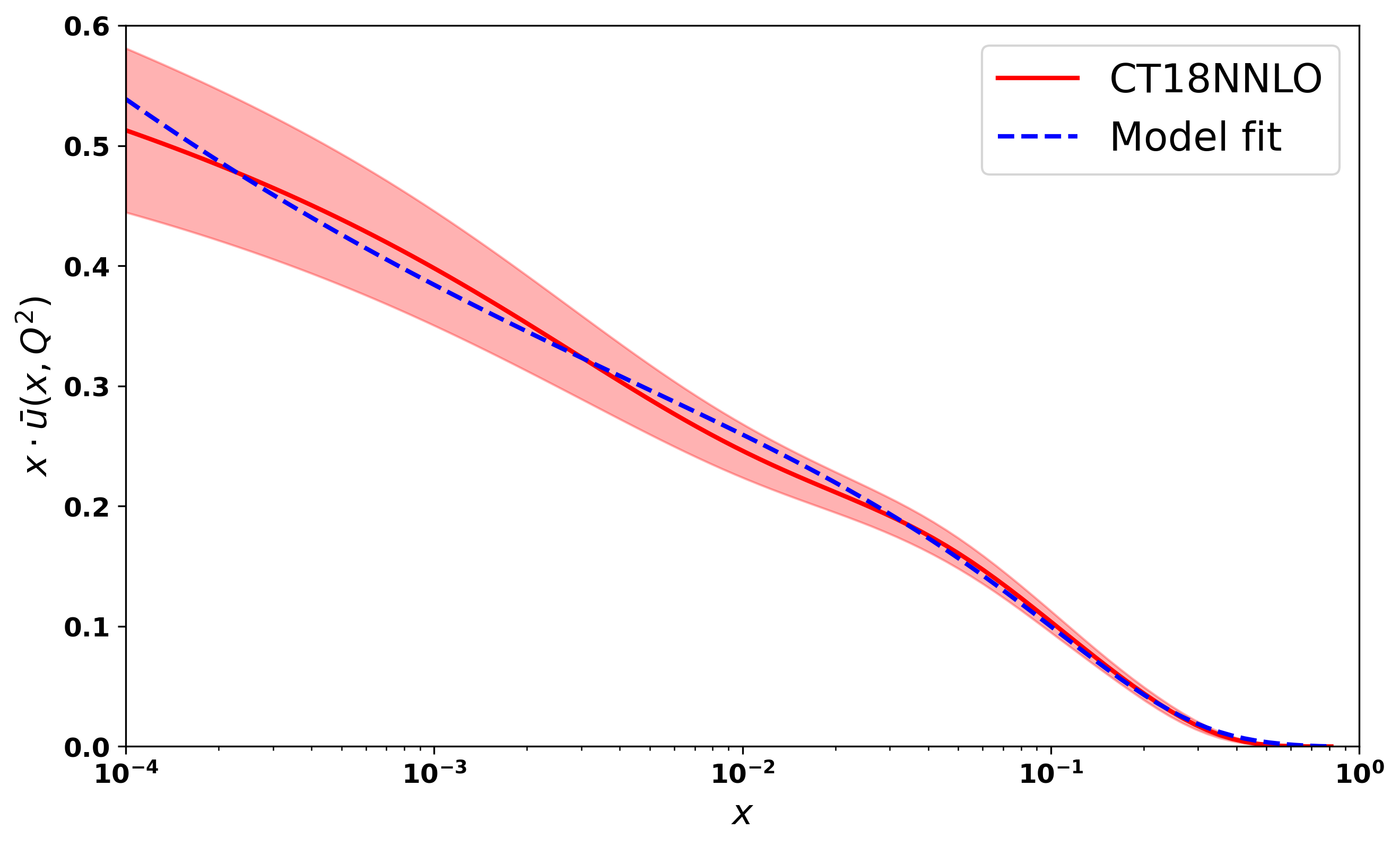
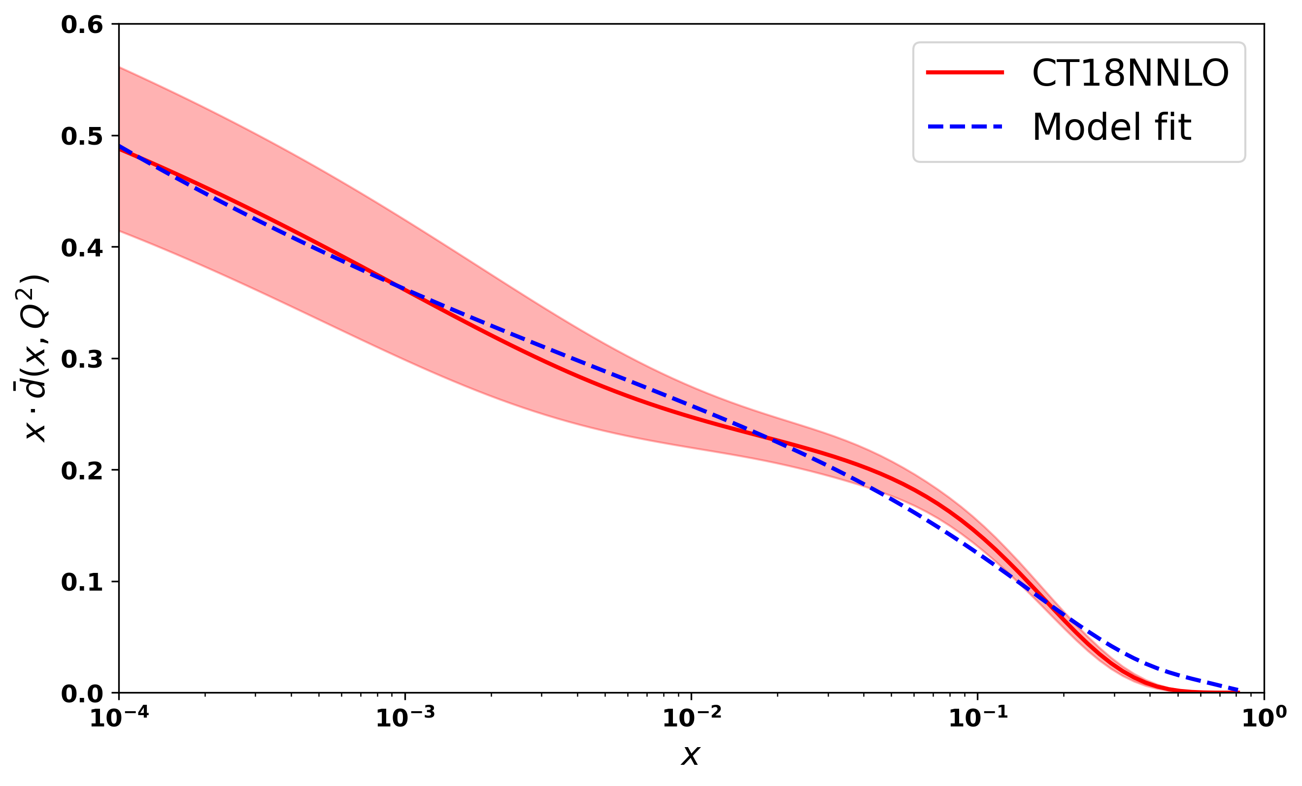
We develop a light-front model of the proton to investigate the twist-3 chiral-even generalized parton distributions (GPDs) of light sea quarks. In this model, the sea quarks are treated as spin- active partons, while the remaining proton constituents are modeled as spin-1 spectators. The momentum wave function, predicted by the soft-wall AdS/QCD, is fitted to the unpolarized parton distribution functions (PDFs) from the CETQ global analysis. Using this fitted distribution, we determine the unknown model parameters. We calculate the twist-3 GPDs and analyze their dependence on the transverse momentum transfer, , and the longitudinal momentum fraction, . Additionally, we explore the Mellin moments and the twist-3 chiral-even PDF, , within this theoretical framework.
I INTRODUCTION
It is an extremely challenging task to understand the internal three-dimensional structure of a proton in terms of its constituent partons (quarks, gluons) [1, 2, 3, 4, 5, 6]. With the help of parton distribution functions (PDFs), the one-dimensional function of the longitudinal momentum fraction and extensive study of the internal structures are carried out. PDFs are forward, diagonal matrix elements that provide a probabilistic interpretation for the operator chosen. Unlike PDFs, GPDs also depend on the squared momentum transfer () and the longitudinal momentum transfer (or skewness ). GPDs are off-forward matrix elements of non-local operators and can be accessed experimentally through processes like deeply virtual Compton scattering (DVCS) [7, 8, 9, 10] or deeply virtual meson production (DVMP) [11, 12, 13, 14]. Experimental data for these processes have been collected by collaborations like H1 [15, 16], ZEUS [15, 17], and fixed-target experiments at HERMES [18, 19], COMPASS [20], and JLab [21, 22]. Considerable progress on the theoretical side has also been observed. Because of the perturbative nature of GPDs, they can’t be directly calculated from the first principle of QCD. Although ongoing lattice calculations will provide more insides. Therefore, model calculations are carried out, such as the MIT bag model [23], the light-front constituent quark model [2, 24, 25, 26], the NJL model [27], the color glass condensate model [28], the chiral quark-soliton model [29, 30], the Bethe-Salpeter approach [31, 32] and the meson cloud model [33, 34].
Parton distribution functions (PDFs) are categorized by their twist, which refers to their order in a expansion, where denotes the hard scale associated with the underlying physical process. While most research on generalized parton distributions (GPDs) has focused on leading-twist contributions, higher-twist GPDs, particularly those of twist-3, remain comparatively under-explored. Nevertheless, twist-3 GPDs provide valuable insights into the partonic structure of hadrons. Notably, there is a connection between quark orbital angular momentum within the nucleon and twist-3 GPDs [6, 35, 36]. The amplitude of deeply virtual Compton scattering (DVCS) at twist-3 can be expressed in terms of twist-3 GPDs through the Compton form factor [37]. Some studies suggest that twist-3 GPDs can also offer insights into the average transverse color Lorentz force acting on quarks [38],[39]. However, experimentally determining higher-twist distributions is challenging, as they are difficult to disentangle from leading-twist contributions. Moreover, higher-twist contributions are typically smaller, owing to suppression factors. The twist-3 GPDs have been investigated in the quark target model [40, 41, 42] and scalar diquark model [42] for the nucleon. The twist-4 proton GPDs were studied within the light-front quark-diquark model (LFQDM) recently [43], and the chiral-even twist-3 GPDs of the proton have also been investigated by the Lattice QCD [44]. The calculations of the twist-3 GPDs chiral-even GPDs of the protons have been carried out in the basis light-front quantization (BLFQ collaboration) [45] with the overlap representations of light-font wave functions.
In this work we have developed a light-front spectator model for proton to study the light sea quarks (), which are considered as spin-, and the remaining spin- particle is considered as a spectator. We have used the momentum wave function predicted by the soft-wall Ads/QCD. The model parameters are determined by fitted unpolarized sea quarks PDF from CTEQ global analysis at scale . We have investigated the behaviors of twist-3 GPDs at different energy scales and x-values. The higher-order Mellin moments of GPDs are also investigated, and we have given the values of Mellin moments in table [2-3], which are calculated from the model under study. In the forward limit and chiral even case, we have only one PDF, , and we have investigated the PDF at different values of ‘’.
In Section I, we present an introduction to the subject matter. Section II provides a detailed calculation of the overlap representation for the twist-3 generalized parton distributions (GPDs). In Section III, we discuss the light-front model used in this study. This is followed by a fit of the unpolarized parton distribution functions (PDFs), calculated from the model, to the CT18NNLO data in order to evaluate the model parameters. In Part III.2 of Section III, we derive the expression for the twist-3 GPDs. Finally, the results and discussion are presented in Section IV.
II CHIRAL EVEN GPDS IN OVERLAP REPRESENTATION
The Generalized Parton Distributions (GPDs) are defined as non-forward matrix elements of the quark-quark correlator function. In light cone coordinate, the quark-quark correlator [46] is commonly written as,
| (1) |
Where is the Dirac bilinear and are the target initial and final state helicities. is the Wilson line, which plays a critical role in ensuring gauge invariance of the nonlocal operator product. It is a path-ordered exponential that connects the quark fields along the light cone, compensating for gauge transformations along the path and maintaining the physical observability of the GPDs. The general definition of is,
| (2) |
Here denotes the path ordering from to . We have to consider the light-cone gauge where . So the value of is , which also makes it color gauge invariant.
The key Dirac bilinears relevant to twist-3 chiral-even generalized parton distributions are given by . Consequently, the parameterization of Equation 1, as provided in [46, 47], for these bilinears is expressed as follows:
| (3) |
| (4) |
The antisymmetric tensor is defined by and is the average proton momentum, is the momentum transfer with and is the skewness parameter. We denote ‘’ as the proton helicity. Since , the parameterization given in equations 3 and 4 can be reduced according to possible helicity combinations. These combinations are listed in Appendix A from equations 36-43. Using these equations, we can derive the explicit formula of the GPDs in overlap representations, which are given below,
| (5) |
| (6) |
| (7) |
| (8) |
| (9) |
| (10) |
| (11) |
| (12) |
III LIGHT FRONT MODEL FOR THE PROTON
In this section to investigate the sea quarks () chiral even generalized parton distribution in proton, we have formulated a light cone spectator model following the steps described in [48]. To generate the sea quark degree of freedom, we have considered the Fock state . The proton is then reduced to a two-particle system. Sea quark is considered an active parton having spin-1/2, and all the other valance quarks and gluons are considered spin-1 spectators.
Throughout the calculations, we have followed the convention . We have considered the frame of reference where the transverse momentum of a proton is zero such that . The two particle Fock state is , with and being the helicities of the sea quark and the spectator. We have used the notation ‘’ for quark and ‘’ for spectator.
The two particle Fock-state expansion can be written as [48] with proton helicity as
| (13) |
The two particle LFWFs of proton with is,
| (14) |
and for we have the following LFWFs,
| (15) |
and represent the mass of proton and spectator. Here is the modified soft-wall Ads/QCD momentum wave function. We have used the wave function that was given in [49] and it has the expression,
| (16) |
The Ads scale parameter is [50], and , , and are model-dependent parameters. They are fixed by fitting unpolarized sea quark PDF with CT18NNLO data set at energy scale . We have considered . The values of the model parameters for the up- and down-sea quarks are given in 1.
III.1 Model parameter fitting
The non-perturbative structures of hadron are studied using parton distributions. Physically, it gives the probability of finding a parton with longitudinal momentum fraction ’. The unpolarized sea quark PDF in our model is expressed as,
| (17) |
| A | |||
|---|---|---|---|
We have followed the procedure provided by [49] to determine the model parameters. In our model, the parameters are and . The parameter is a free parameter, and it describes the amplitude of sea quarks PDF in the region. The parameter controls the low value, and the parameter controls the high value. In fig 1, the top figure is for and the bottom figure is for . Since the model relies on only three parameters, it has a notable advantage.
III.2 Chiral even GPDs at zero skewness
The quark-quark correlator, as presented in [43], is expressed in the overlap representation at as,
| (18) |
In this context, and denote the initial and final helicities of the sea quark, respectively. In the overlap representation, is treated as a two-dimensional complex vector, defined by . The expression
represents the spinor product associated with higher-twist Dirac matrices. The Dirac matrices within the light-cone formalism are comprehensively detailed in [51, 52]. The initial and final transverse momenta of the struck sea quark are,
| (19) |
At zero skewness (), only four chiral GPDs remain, as shown using the symmetry properties of GPDs in [45]. Therefore, the chiral-even GPDs of sea quarks can be derived from equations 5-12,
| (20) |
| (21) |
| (22) |
| (23) |
The light-front wave functions from equations (14) and (15) are applied to the generalized parton distributions (GPDs) in equations (20), (21), (22), and (23). Subsequently, the integration over the transverse momentum is carried out to derive the analytical expressions of the GPDs. The limit of the integration is from to . In this calculations we have some used standard Gaussian integrals. These integrals are listed in appendix B.
IV Result and Discussion
In this section we have presented the analytical results of twist-3 chiral even GPDs of light sea quarks in the proton at zero skewness in the light front spectator framework. We have also calculated the numerical results of Mellin moments as well as twist-3 on the gravitational form factor . The twist-3 PDF () is investigated, and we have also examined the Burkhardt-Cottingham sum rule [53] for and .
IV.1 Twist-3 chiral even GPDs
We have analytically solved GPDs within our model using the overlap representation presented in equations (26)-(29). Since , we have investigated the GPDs as a function of and . In our calculation we have found that and are non-zero and all other chiral even GPDs are zero, which is consistent with [45].
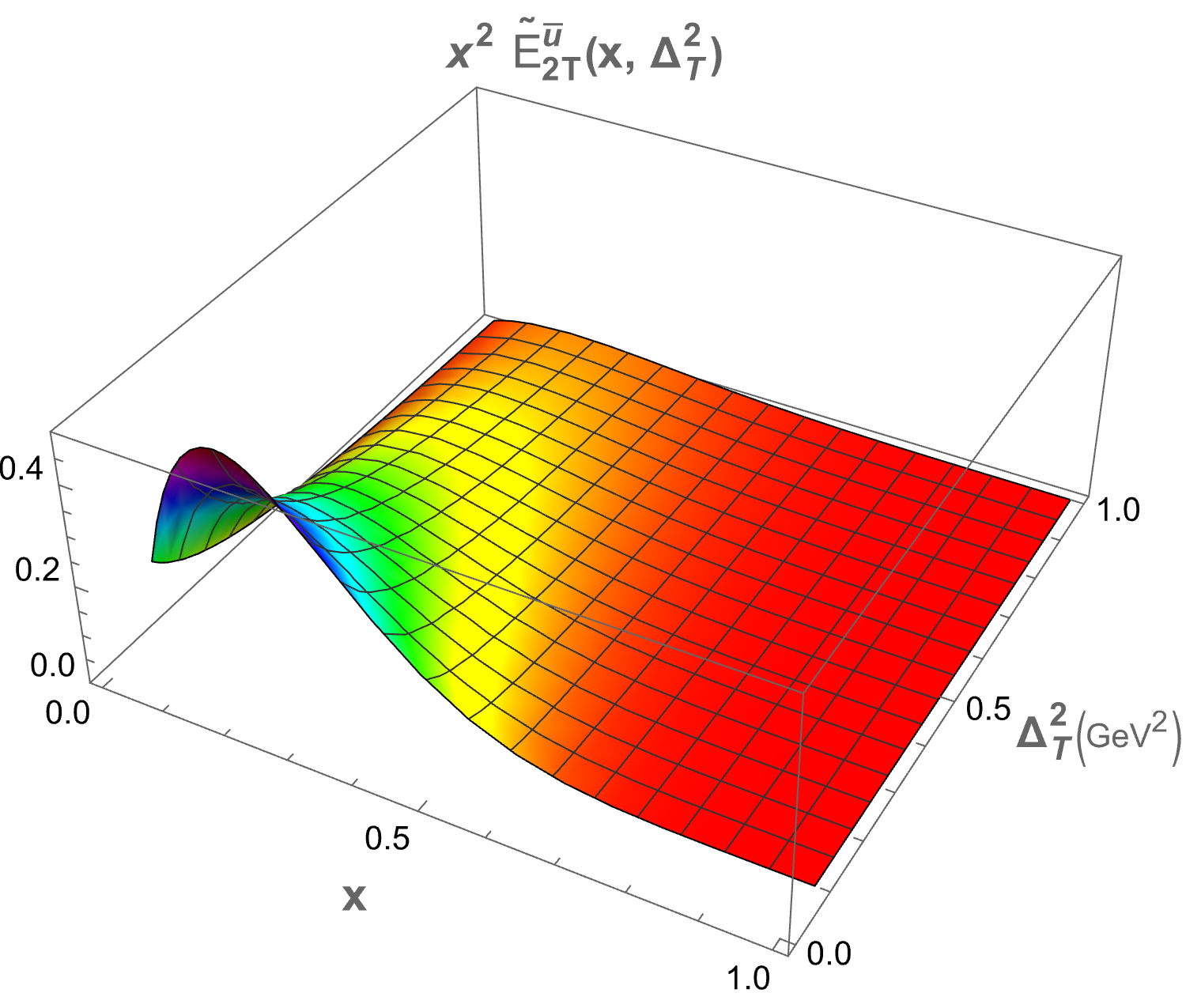
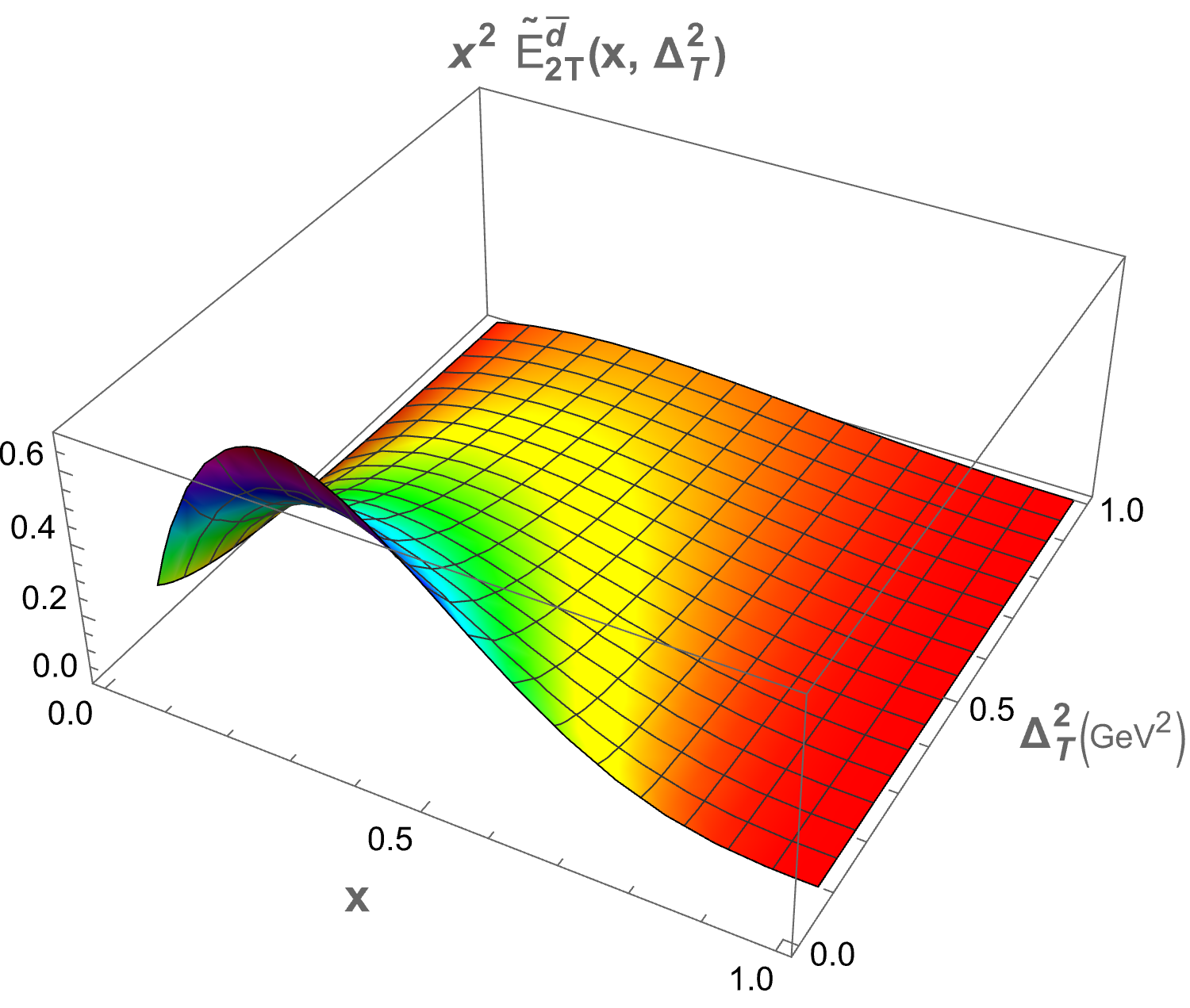
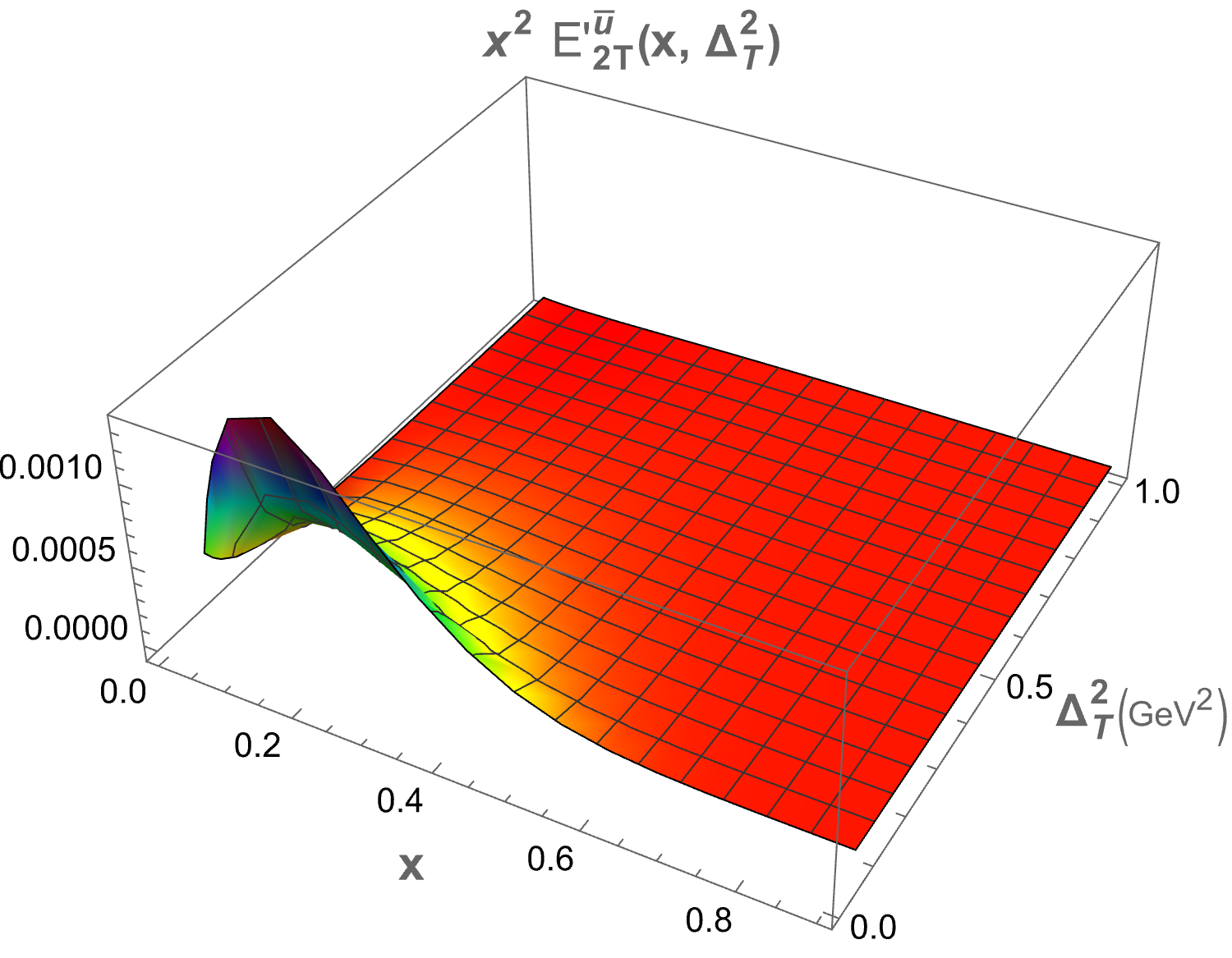
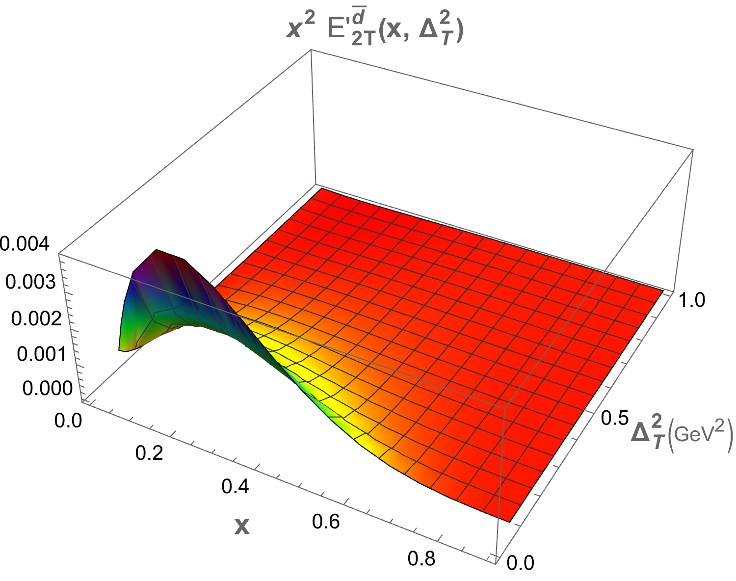
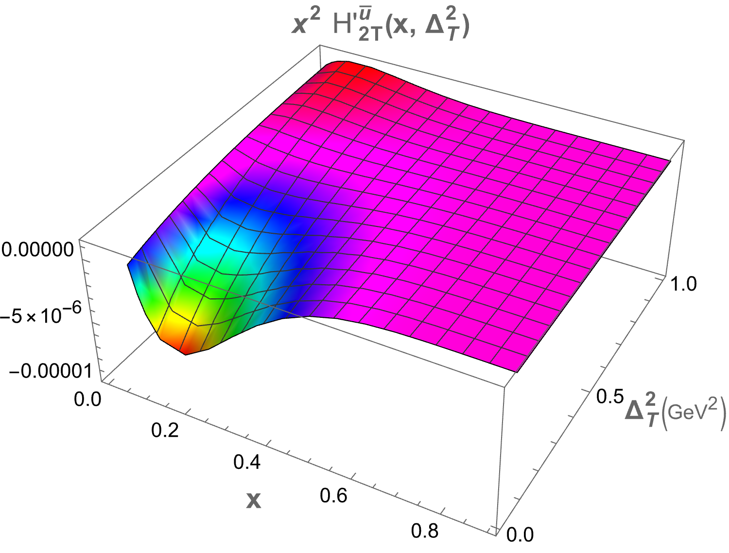
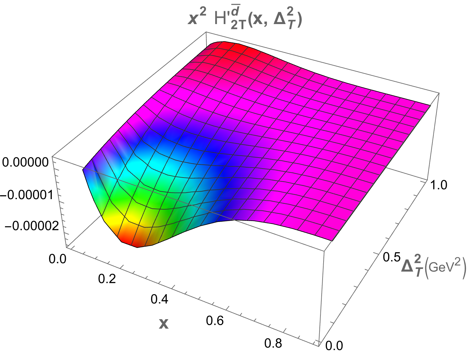
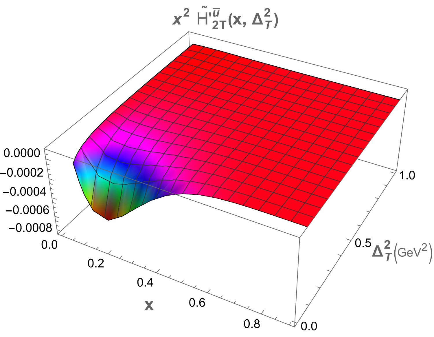
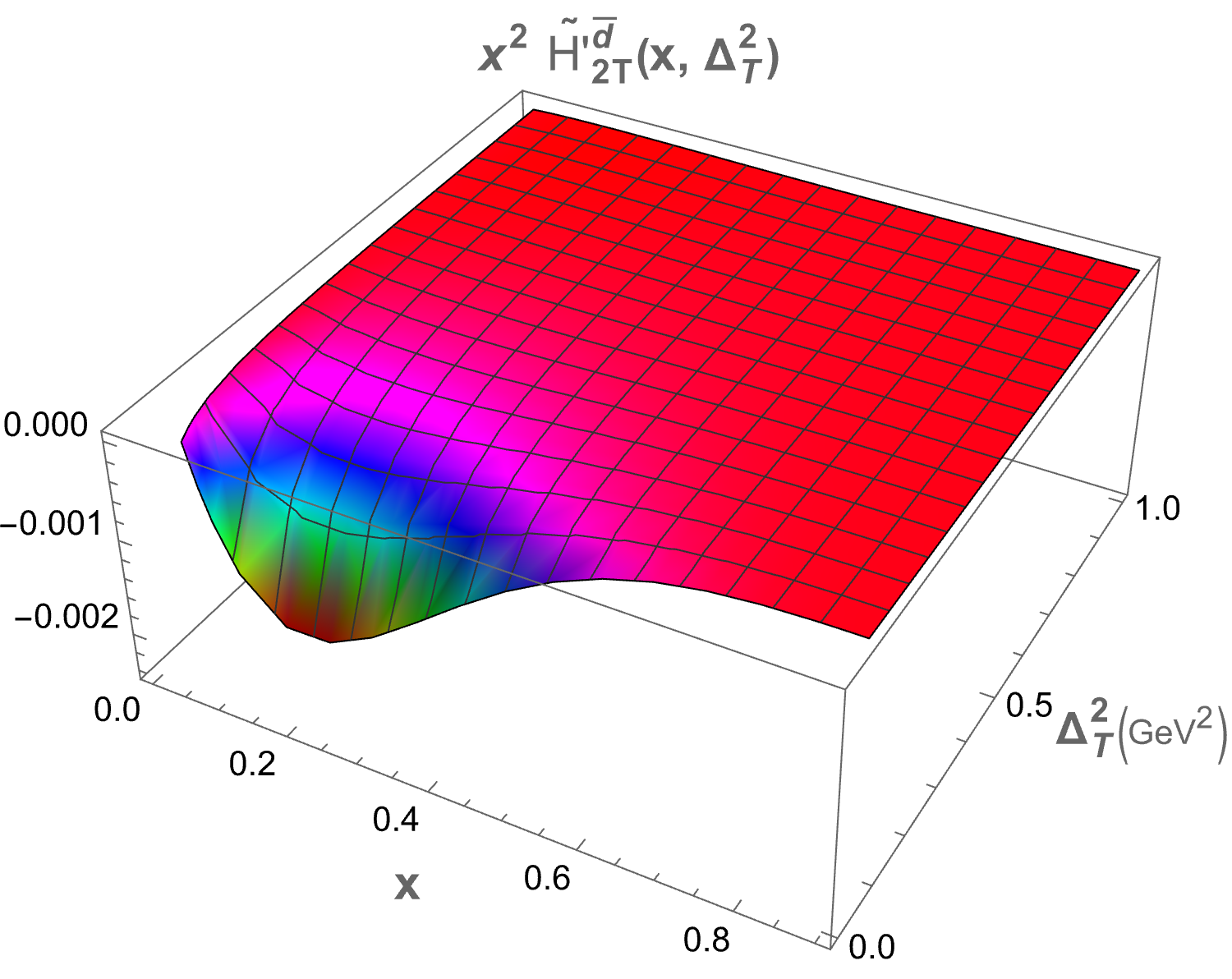
The only structure that remains at zero skewness is . In Figure 2, we present plots of as functions of and for both sea quark flavors. A symmetry is observed for the and flavors, which arises due to the longitudinal polarization of the proton. The 3D plot for shows a peak at , while for the peak occurs at . This difference in peak positions is attributed to the presence of the quark mass term in the GPDs expression. Both plots exhibit a Gaussian-like nature. The structures , , and , which correspond to the components, also survive at zero skewness. Figure 3 displays the 3D plots of these structures against and . The function demonstrates the same Gaussian characteristics as . For , the peak is located at , while for , it is found at . Notably, and exhibit similar but negative distributions. The quantity decreases more sharply than in the energy range . Specifically, peaks at for and for . For , the peaks occur at for and for .
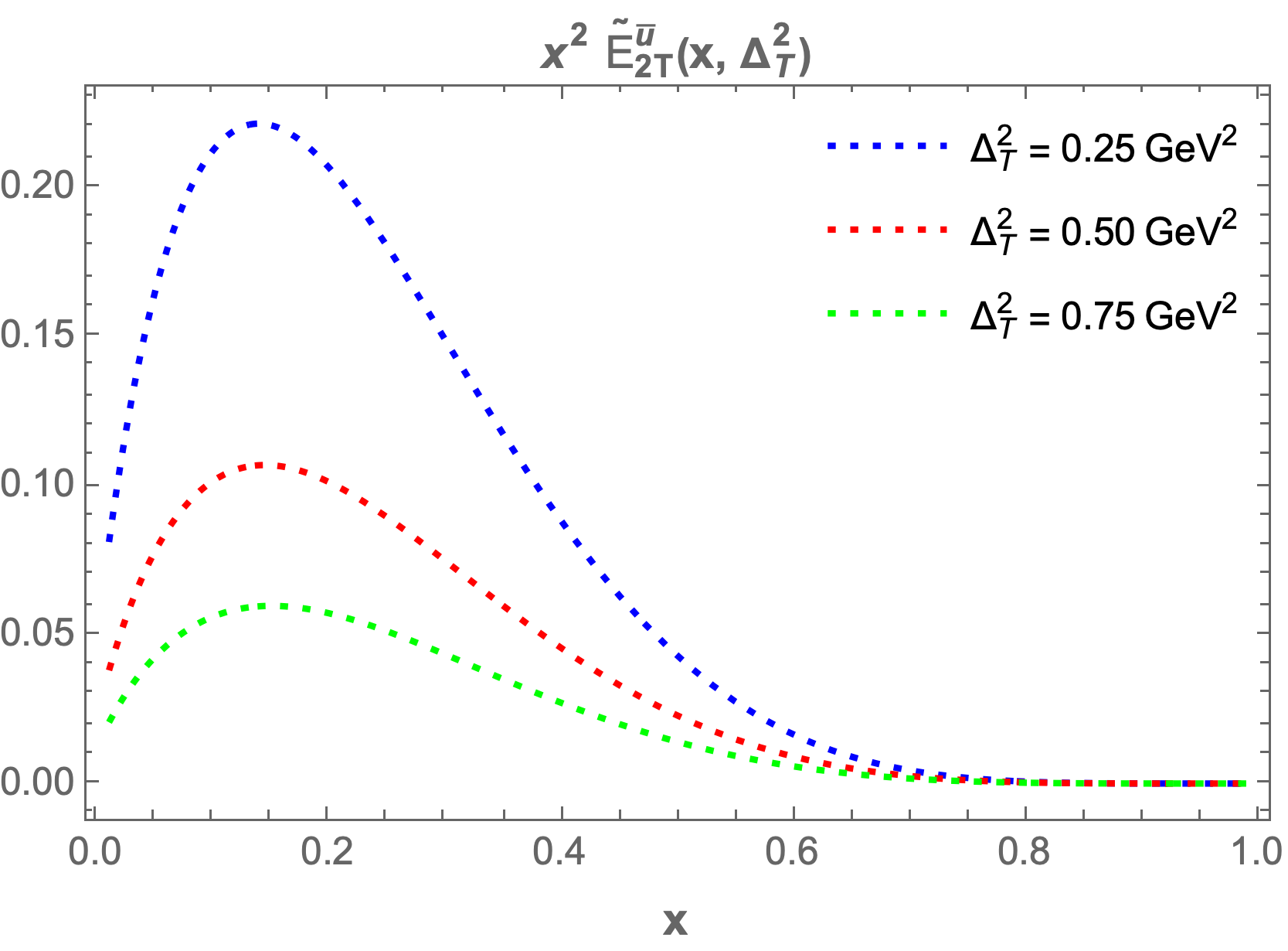
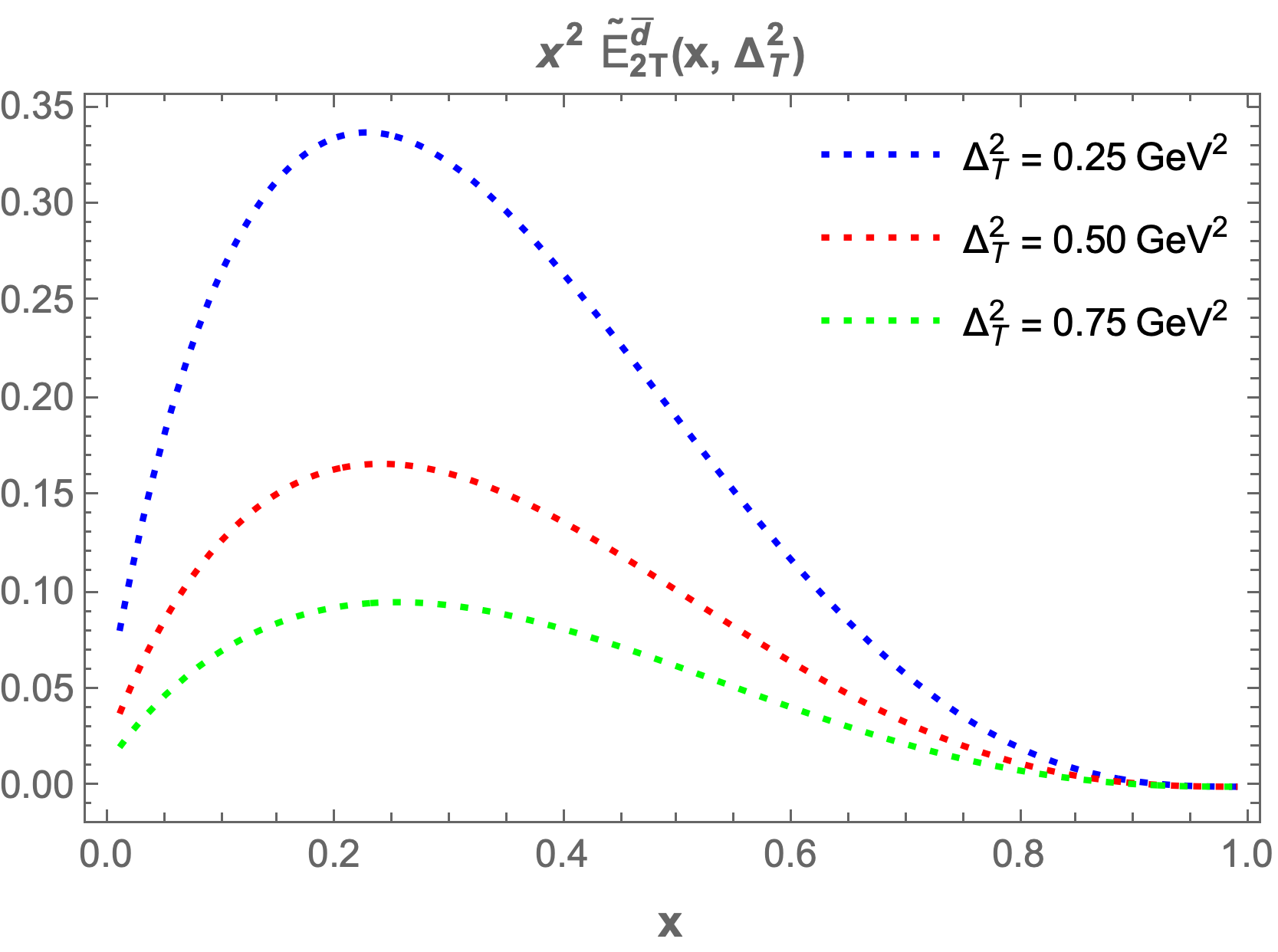
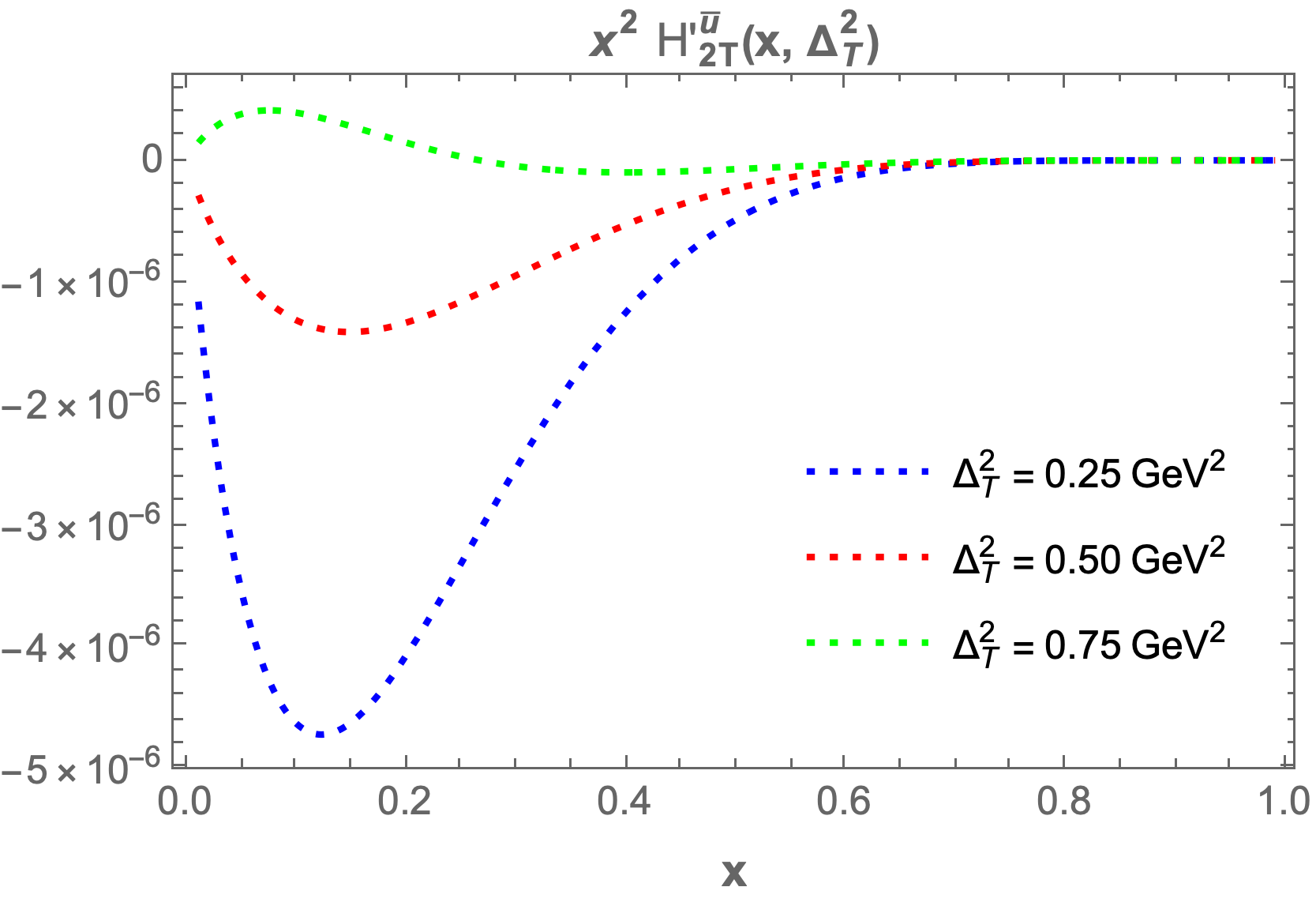
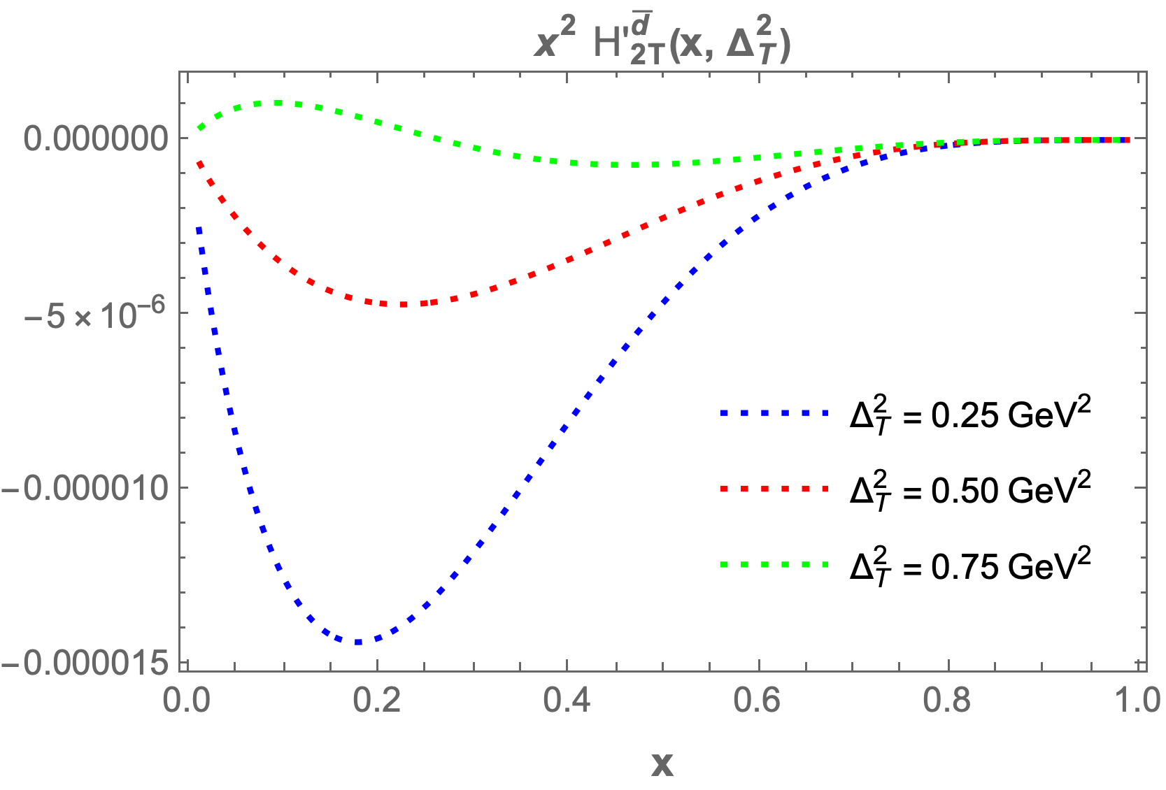
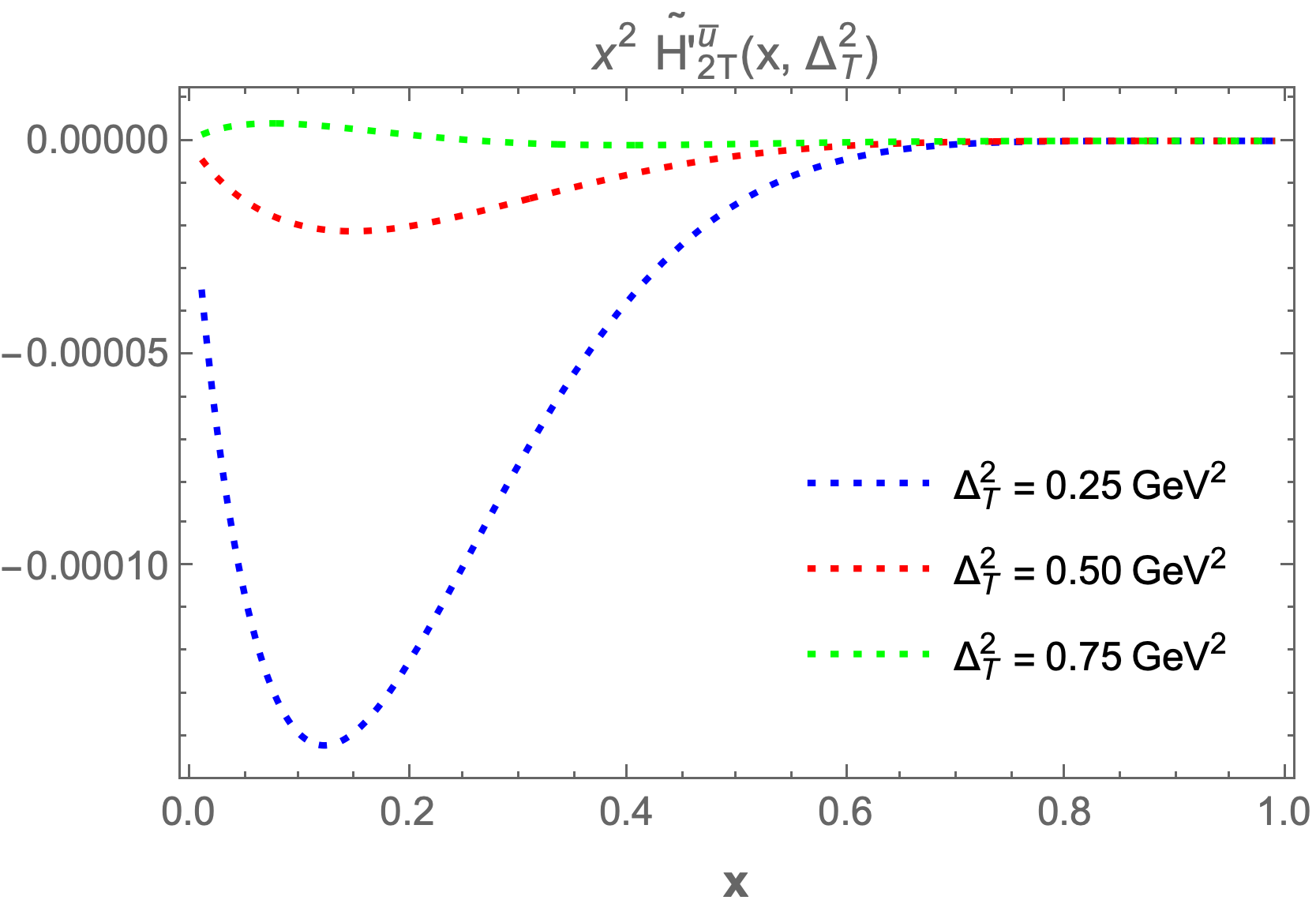
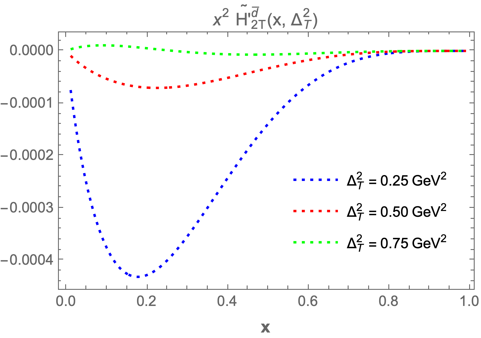
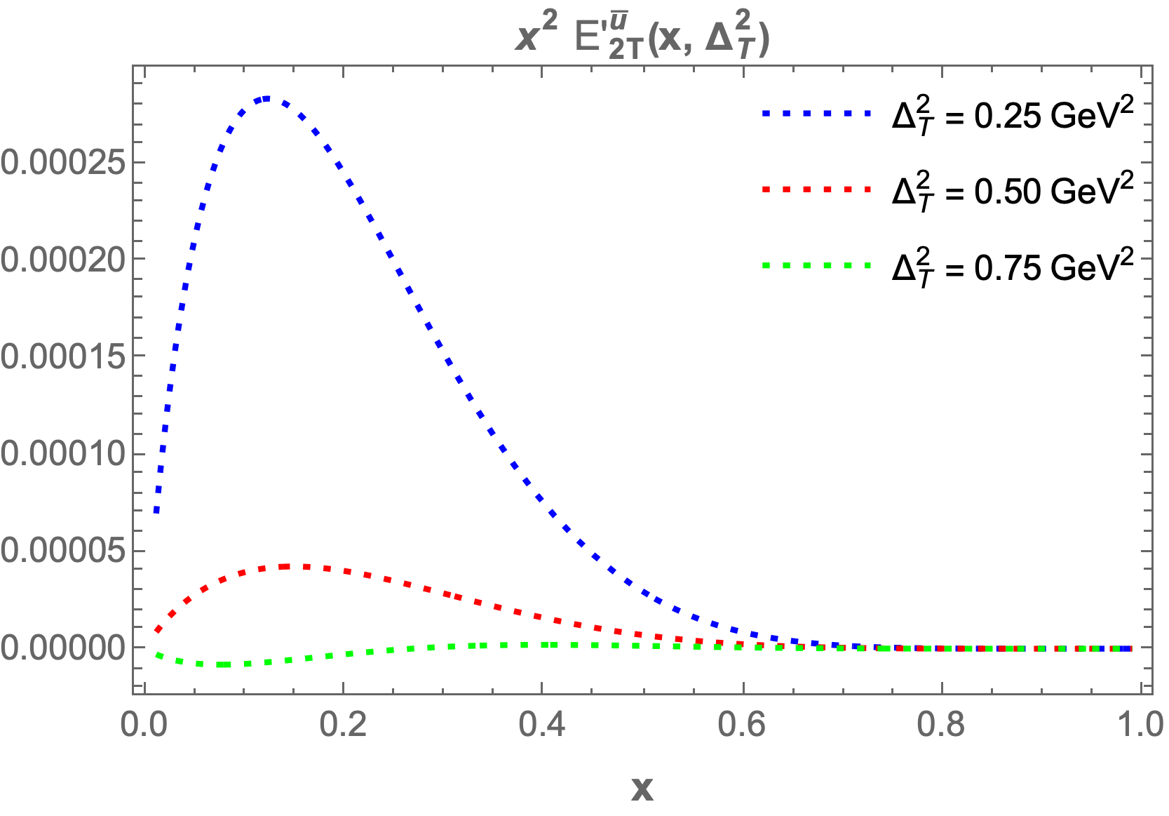
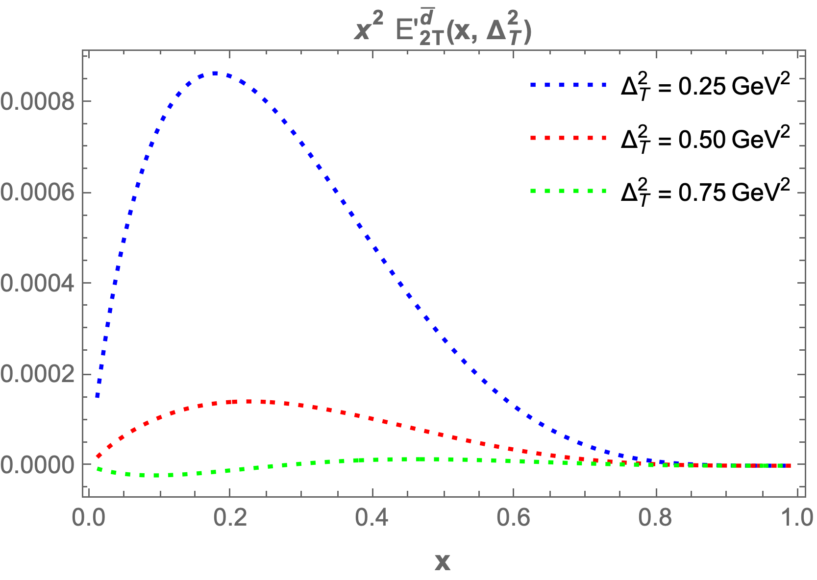
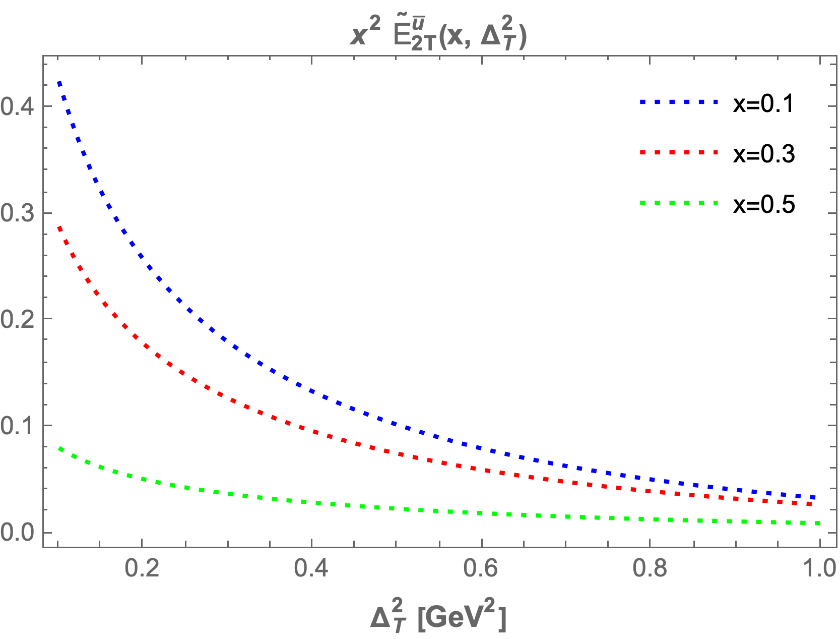
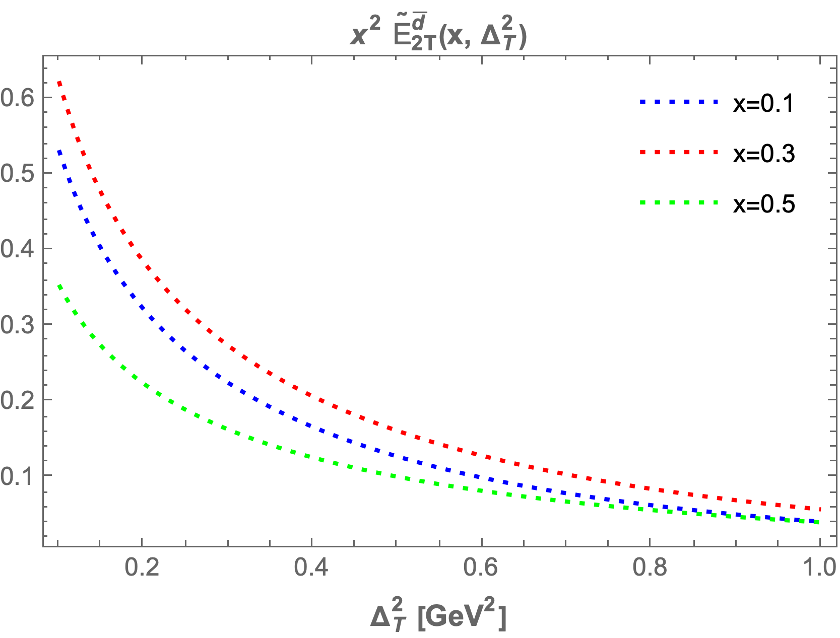
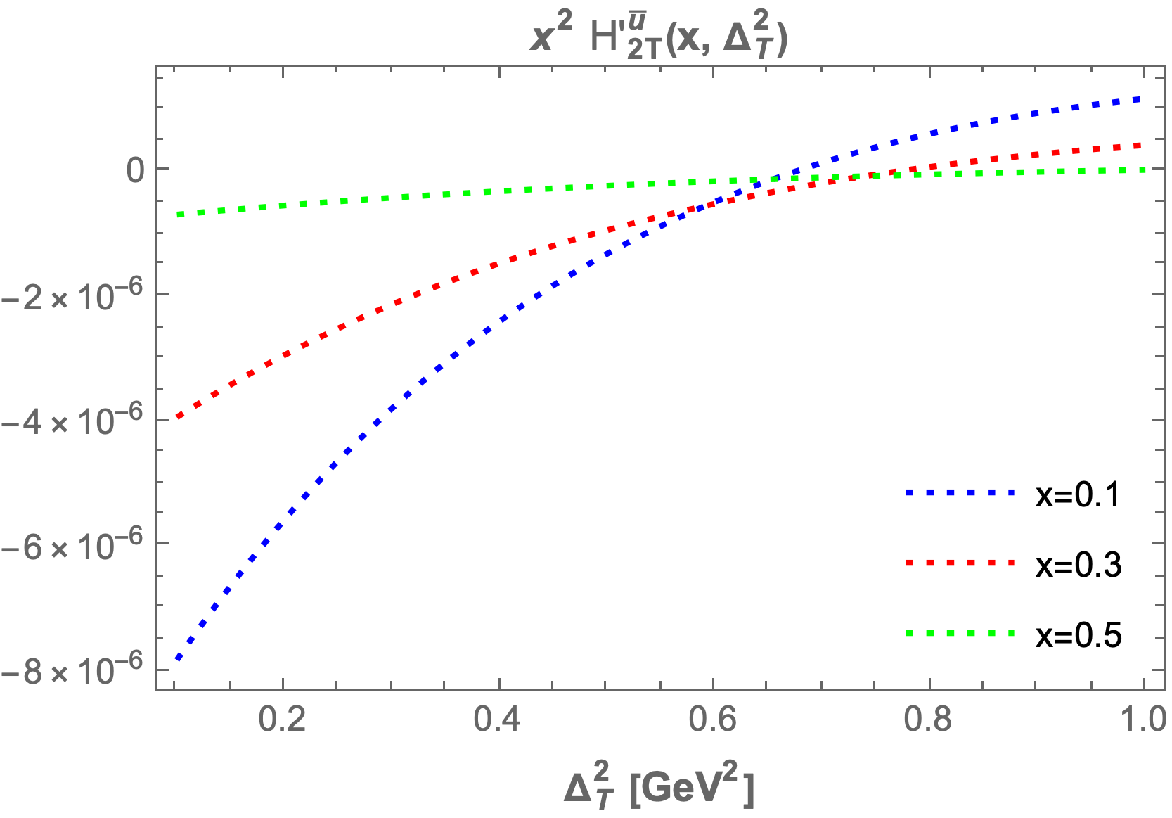
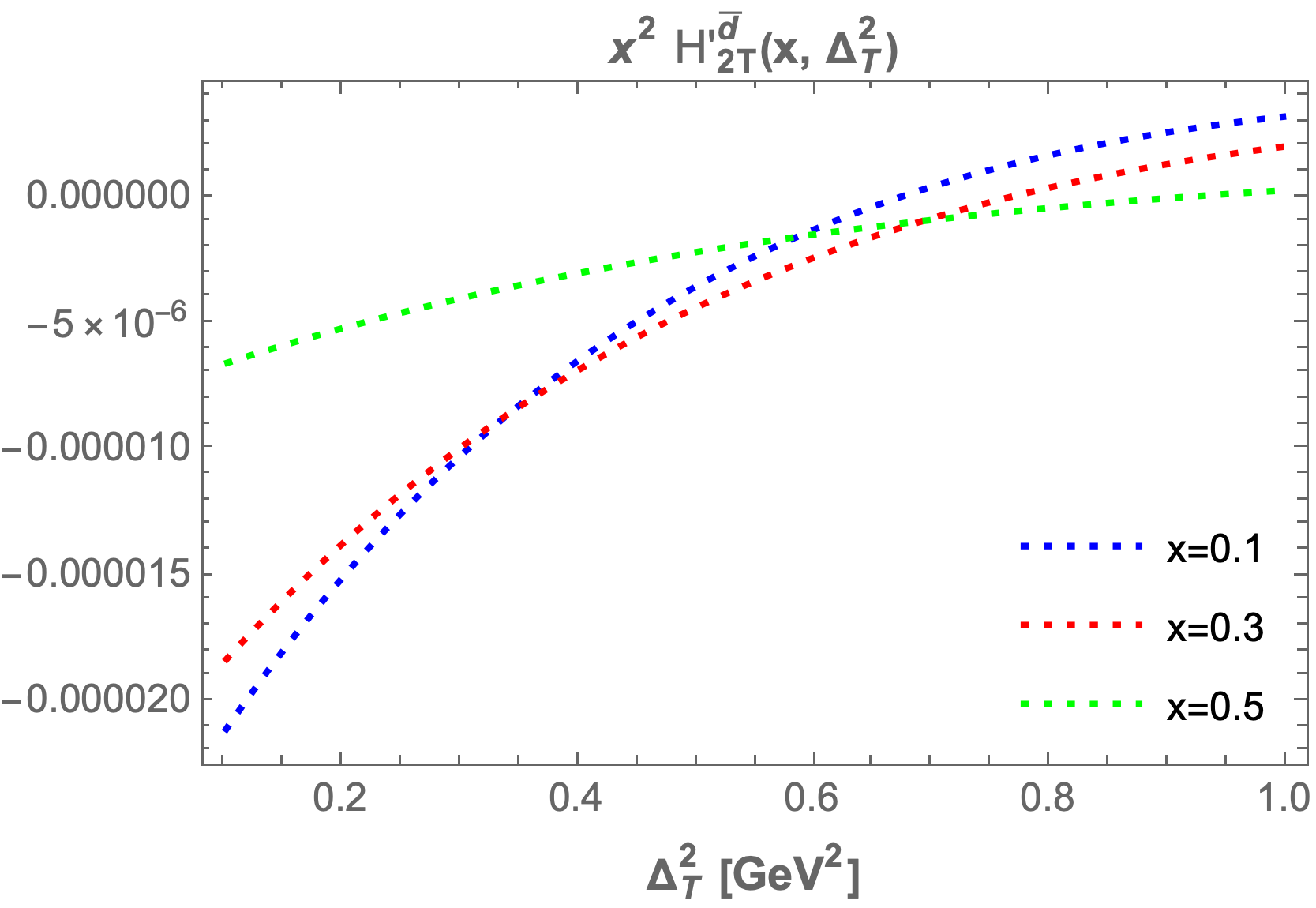
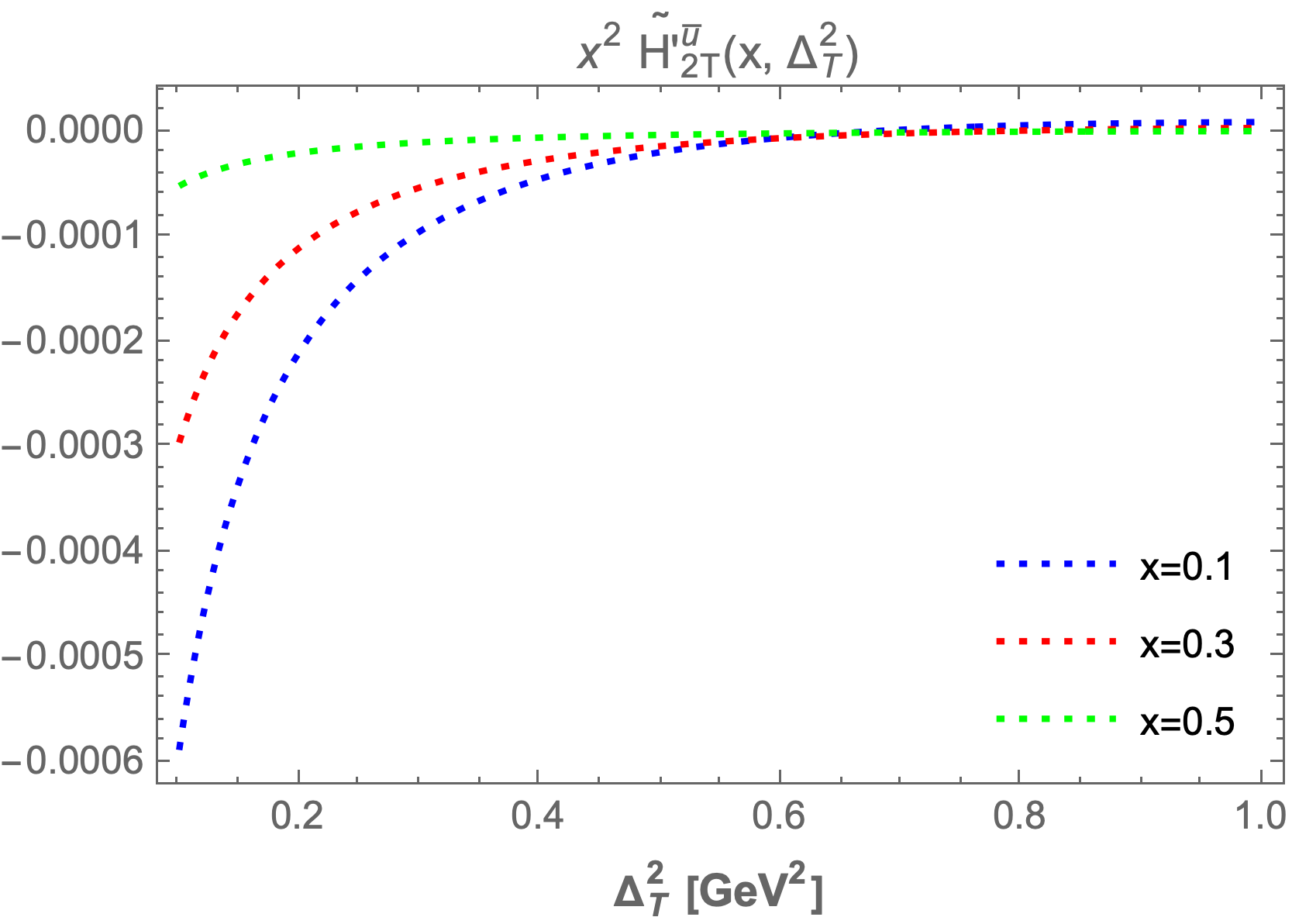
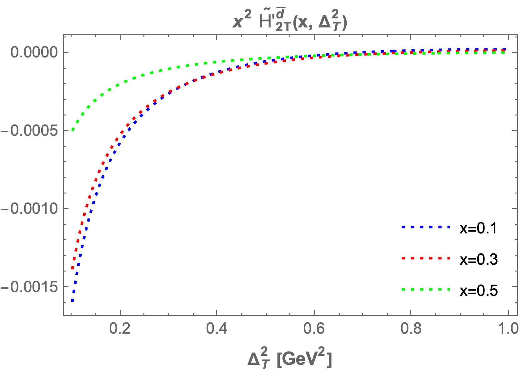
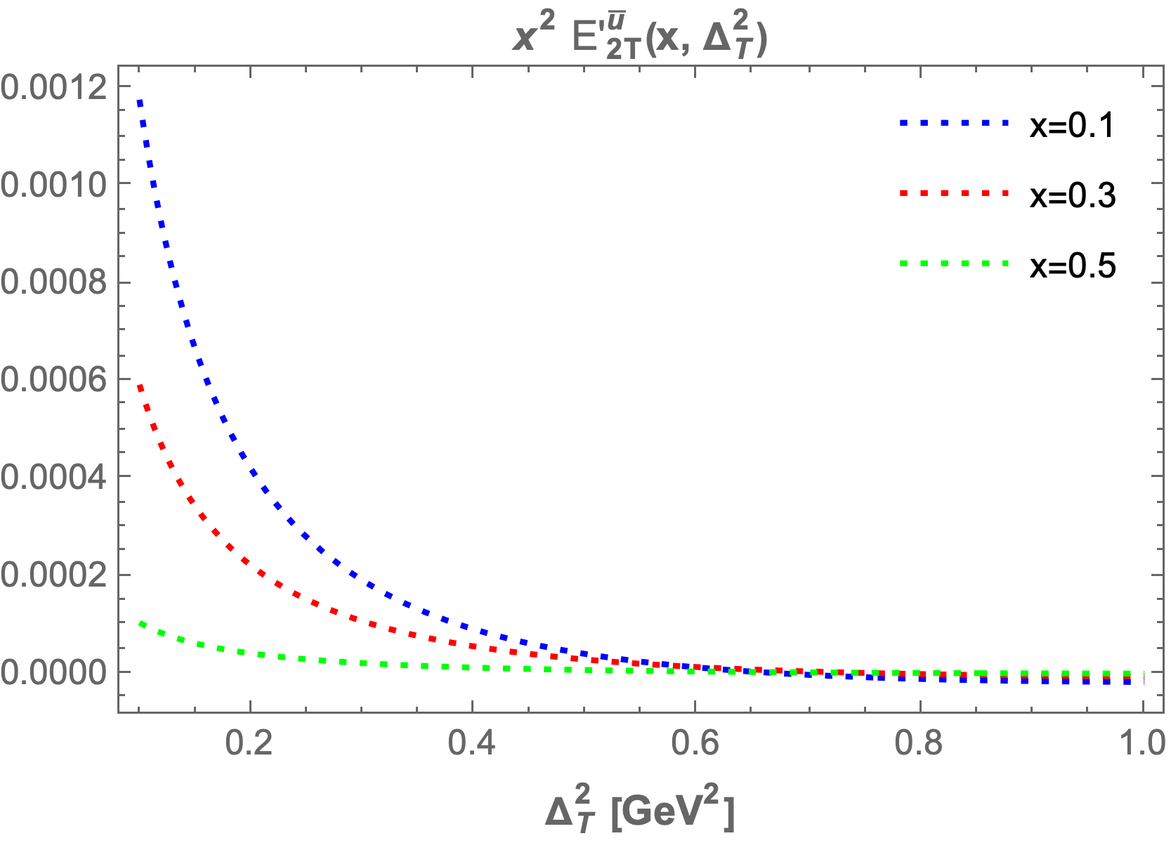
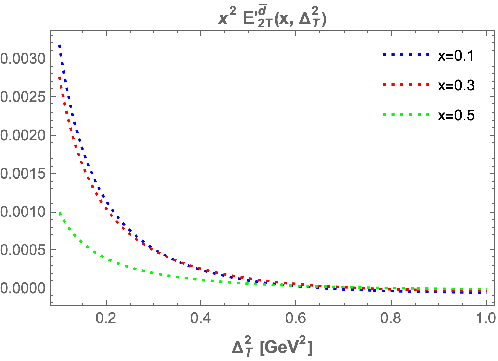
The chiral-even generalized parton distributions (GPDs) , , , and are plotted at fixed values of transverse momentum transfer and longitudinal momentum fraction to enhance our understanding. In Figure 6, we present the GPDs at fixed values of , , and , where the left column figures correspond to and the right column figures correspond to .
We observe that and increase as the longitudinal momentum increases, peaking between and before beginning to decrease. The highest maxima occur at lower values of , while for larger values of , the GPDs become negligible. A similar pattern is observed for and ; however, they begin to decrease and reach a minimum in the range of to for both sea quarks and , before increasing again. For larger values of , the GPDs approach zero.
We also plot the GPDs at fixed values of , , and while varying from to . Key observations indicate that as increases, the GPDs ( and ) fall sharply and asymptotically approach zero. With increased fixed values of , the GPD values become negligible. Similar trends are noted for the other GPDs, which also start increasing sharply and then asymptotically approach zero.
IV.2 Mellin moments of twist-3 GPDs
Mellin moments are powerful tools that relate the internal structure of hadrons with measurable quantities like form factors and parton distribution functions (PDFs). The Mellin moments of GPDs can be linked to generalized form factors (GFFs). Mathematically, they are defined as,
| (24) |
We have numerically evaluated the Mellin moments using Eq. 24 at zero skewness. The generalized parton distributions (GPDs) under investigation are denoted as . The zeroth Mellin moment () corresponds to the form factor associated with the total momentum carried by the quarks. Higher Mellin moments () can give access to various components of the angular momentum and the distribution of forces inside the hadron. In Table 2, the calculations are presented for the distribution for and . Similarly, Table 3 shows the results for the distribution for and . The Mellin moment calculation can be tested in future lattice calculations and high-precision experiments to validate the model.
| 3.03478 | 0.548378 | 0.119956 | |
| -0.00379745 | -0.000647706 | -0.000130139 | |
| -0.0000506056 | |||
| 0.00759489 | 0.00129541 | 0.000260278 |
| 4.9224 | 1.03145 | 0.277907 | |
| -0.0127497 | -0.00242491 | -0.000568928 | |
| -0.000169905 | -0.0000323149 | ||
| 0.0254994 | 0.00484982 | 0.00113786 |
To study the gravitational form factors we have adopted a different parameterization given in [54],
| (25) |
By comparing them with the ones in equation 3, we have the following relations between the GPDs [54],
| (26) | ||||
| (27) | ||||
| (28) | ||||
| (29) |
However, at zero skewness (), only one of the above GPD survives. So we are left with the only equation 28. The first Mellin moment is expressed as,
| (30) | ||||
| (31) |
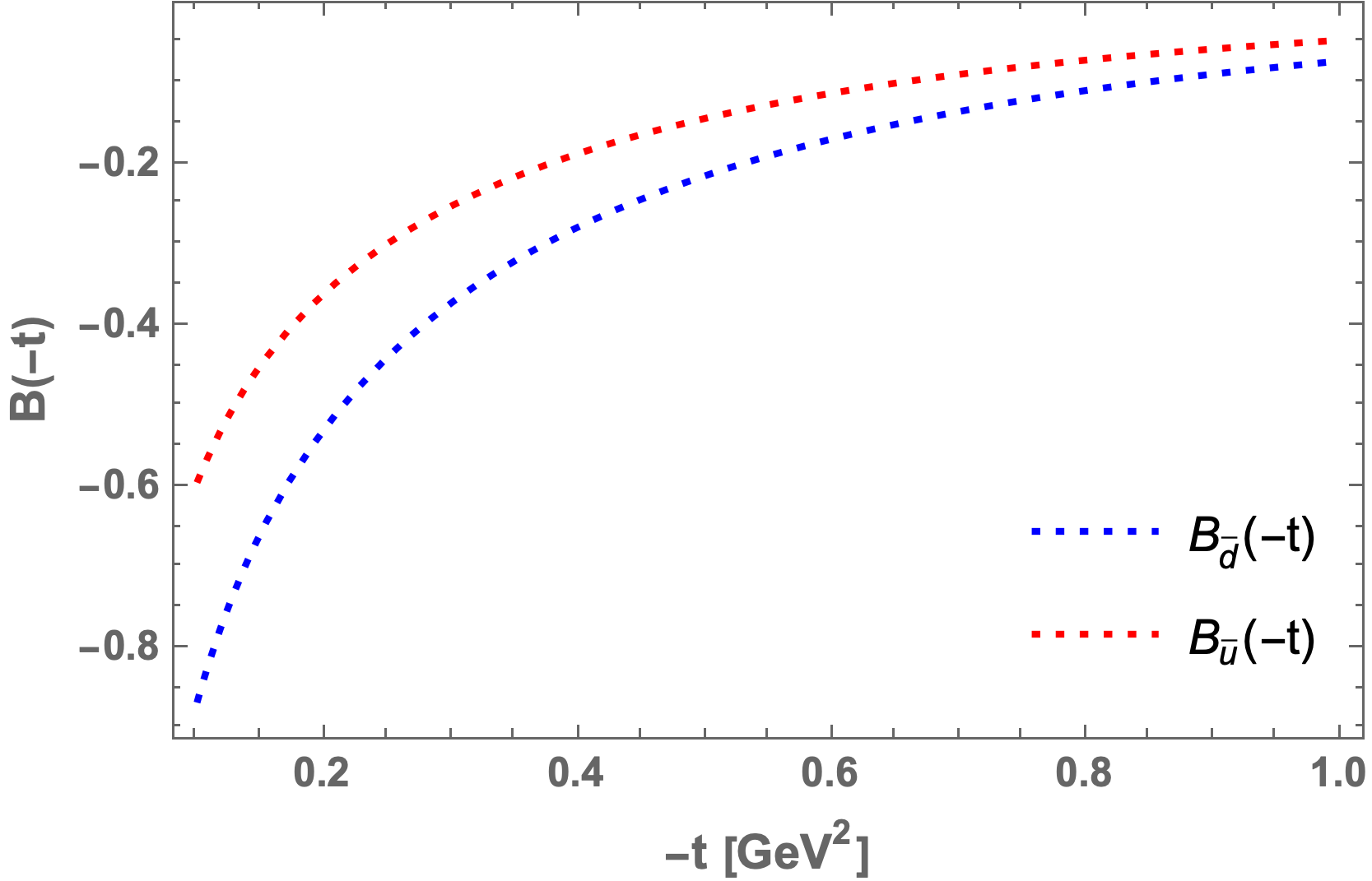
Using Ji’s sum rule [6], which relates the total angular momentum with GPDs, we can investigated the twist-3 contribution of sea quarks to the total angular momentum. From figure 4, we have observed that with increasing momentum transfer, asymptotically approaches zero. So at large momentum transfer the contribution from twist-3 GPDs to orbital angular momentum (OAM) is negligible. At , and . Hence, at low energy transfer has larger contributions to OAM of proton than .
IV.3 PDF limit
The PDFs are interpreted as parton densities corresponding at a longitudinal momentum fraction . The PDFs are mathematically defined by quark-quark correlator,
| (32) |
In this work, we focus solely on twist-3 chiral-even GPDs. Therefore, we consider the structures and . In the forward limit and at zero skewness, there is only one chiral-even GPD that has a PDF structure. This is given by:
| (33) |
and is connected to the twist-3 GPD . The expression that connects the two is given by,
| (34) |
Equations 23 and 34 show that measures the traverse spin distribution for quarks. It’s very hard to experimentally measure the value of . In this work we have calculated the theoretical values for and also plotted the evolution of with respect to at different values of transverse momentum transfer ‘’ in figure 5.
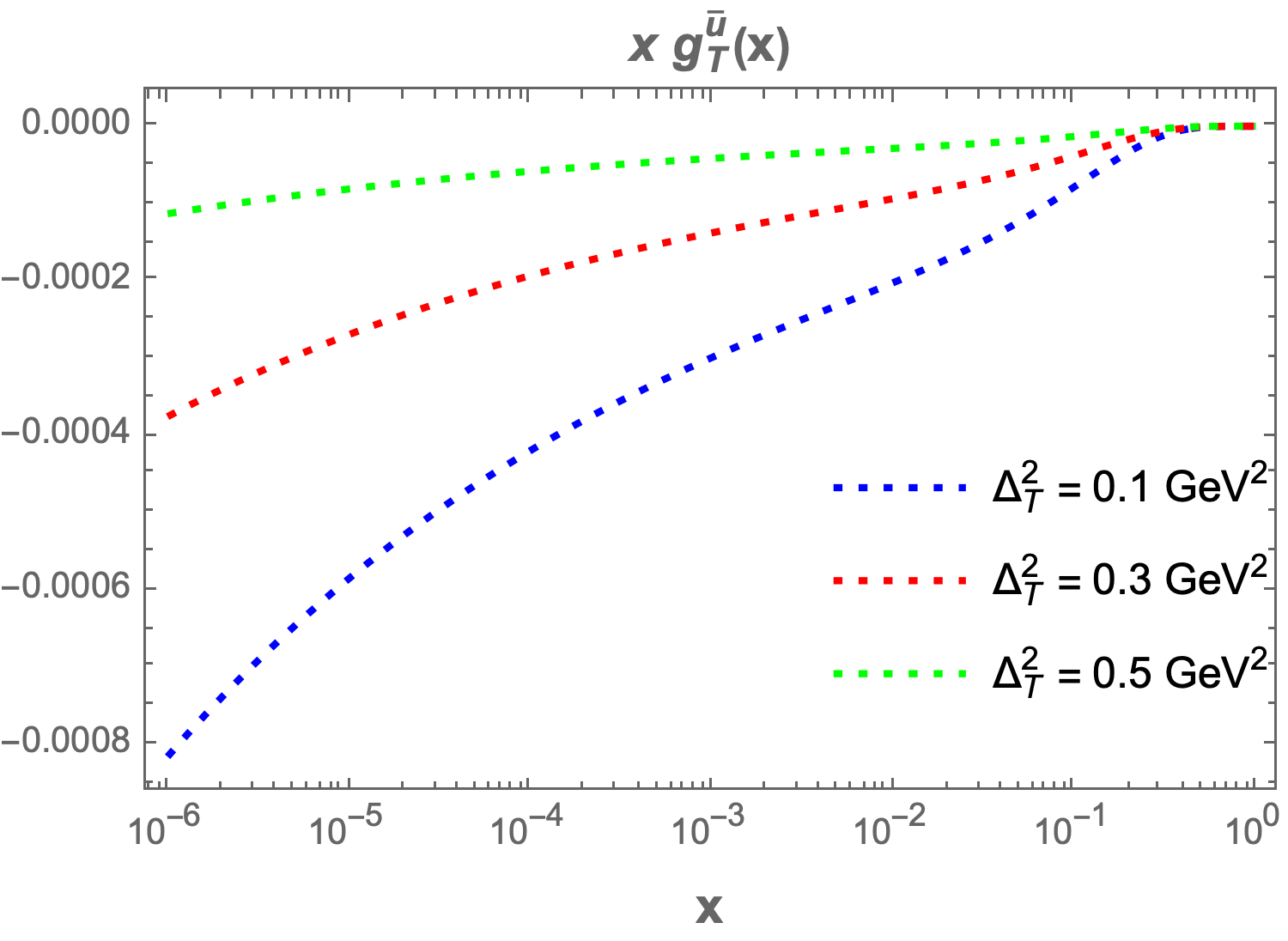
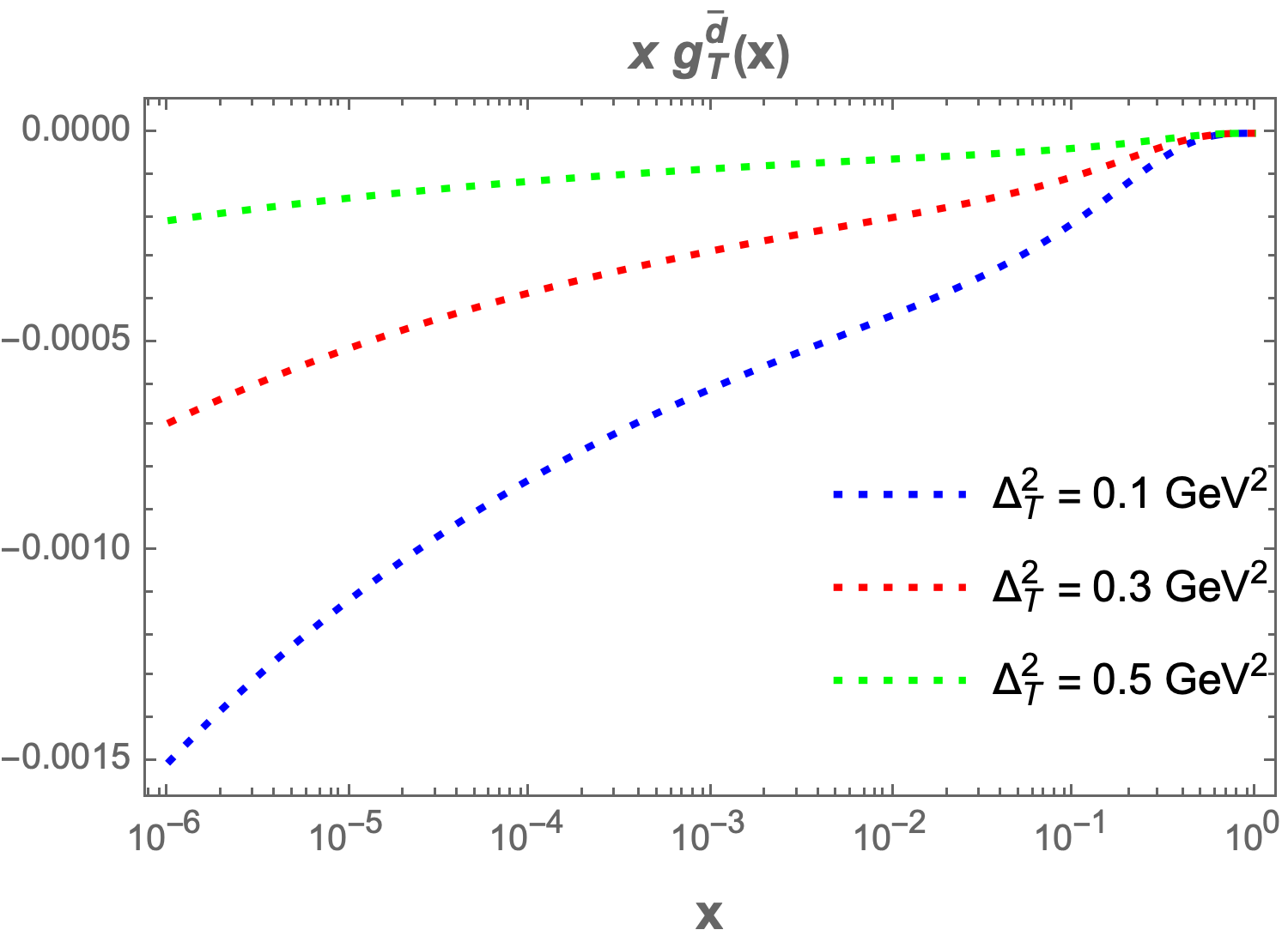
Our key observation is that the as a function of decreases as the value of increases. For larger values of , PDF becomes negligible, and the magnitude of is larger than . Although doesn’t have direct partonic probability interpretation, it is sensitive to the quark-gluon correlation [55]. The Burkhardt-Cottingham sum rule [53] relates the twist-3 PDF and twist-2 PDF . The expression of the sum rule is,
| (35) |
Validation of this sum rule implies that the contributions of quark spin to the proton spin, under different polarization states, are identical. We have numerically checked the sum rule. But in our model, we have observed that both and violate the sum rule because of the presence of the quark mass terms [56]. This violation also indicates the breaking of rotational invariance in our model.
V CONCLUSION
In this paper, we investigate the twist-3 chiral-even generalized parton distributions (GPDs) of light sea quarks, specifically and , within the light-front spectator model framework. Utilizing the parameterizations outlined in [21, 47], we express the GPDs through light-front wave functions. Our formalism closely follows the basis light-front quantization (BLFQ) approach presented in [45]. We provide a comprehensive analysis of two-dimensional (2D) and three-dimensional (3D) representations of the GPDs to illustrate their behavior across various values of transverse momentum transfer, , and longitudinal momentum fraction, . Additionally, we explore higher-order Mellin moments and, by applying different GPD parameterizations, investigate the gravitational form factor for and quarks. Lastly, we examine the twist-3 parton distribution function (PDF) for the sea quarks.
The investigation of higher-twist generalized parton distributions (GPDs) of sea quarks is less explored compared to the extensive research on leading-twist GPDs. In future studies, we intend to compute higher-twist GPDs for sea quarks at non-zero skewness (), accounting for contributions from higher Fock states. The study of non-zero skewness is particularly pertinent to the twist-3 cross-section of deeply virtual Compton scattering (DVCS) [37], which will be examined in upcoming experiments at the Electron-Ion Collider (EIC) and the Electron-Ion Collider in China (EicC) [57]. This research will also enable us to investigate the relationships between higher-twist GPDs and orbital angular momentum distributions. Understanding higher-twist effects will yield qualitative insights into the internal structure of the proton and contribute to addressing longstanding questions, such as the proton spin puzzle and the proton mass problem.
Appendix A
The parametrization of the quark-quark correlator is given in equations 3 and 4. According to the initial and final helicity of the particle, we can reduce these equations. For , we have
| (36) |
| (37) |
| (38) |
| (39) |
Similarly for we have the following,
| (40) |
| (41) |
| (42) |
| (43) |
Appendix B
Some standard Gaussian integrals that are used in our calculations are,
| (44) | ||||
| (45) | ||||
| (46) | ||||
| (47) |
References
- Deur et al. [2019] A. Deur, S. J. Brodsky, and G. F. De Téramond, The spin structure of the nucleon, Reports on Progress in Physics 82, 076201 (2019).
- Boffi and Pasquini [2007] S. Boffi and B. Pasquini, Generalized parton distributions and the structure of the nucleon, La Rivista del Nuovo Cimento 30, 387 (2007).
- Kuhn et al. [2009] S. Kuhn, J.-P. Chen, and E. Leader, Spin structure of the nucleon—status and recent results, Progress in Particle and Nuclear Physics 63, 1 (2009).
- Filippone and Ji [2001] B. Filippone and X. Ji, The spin structure of the nucleon, in Advances in nuclear physics (Springer, 2001) pp. 1–88.
- Aidala et al. [2013] C. A. Aidala, S. D. Bass, D. Hasch, and G. K. Mallot, The spin structure of the nucleon, Reviews of Modern Physics 85, 655 (2013).
- Ji [1997a] X. Ji, Gauge-invariant decomposition of nucleon spin, Physical Review Letters 78, 610 (1997a).
- Ji [1997b] X. Ji, Deeply virtual compton scattering, Physical Review D 55, 7114 (1997b).
- Radyushkin [1996] A. Radyushkin, Scaling limit of deeply virtual compton scattering, Physics Letters B 380, 417 (1996).
- Belitsky et al. [2002] A. V. Belitsky, D. Mueller, and A. Kirchner, Theory of deeply virtual compton scattering on the nucleon, Nuclear Physics B 629, 323 (2002).
- Hashamipour et al. [2020] H. Hashamipour, M. Goharipour, and S. S. Gousheh, Determination of generalized parton distributions through a simultaneous analysis of axial form factor and wide-angle Compton scattering data, Phys. Rev. D 102, 096014 (2020), arXiv:2006.05760 [hep-ph] .
- Goloskokov and Kroll [2007] S. Goloskokov and P. Kroll, The longitudinal cross section of vector meson electroproduction, The European Physical Journal C 50, 829 (2007).
- Goloskokov and Kroll [2008] S. Goloskokov and P. Kroll, The role of the quark and gluon gpds in hard vector-meson electroproduction, The European Physical Journal C 53, 367 (2008).
- Goloskokov and Kroll [2010] S. V. Goloskokov and P. Kroll, An attempt to understand exclusive + electroproduction, The European Physical Journal C 65, 137 (2010).
- Goloskokov and Kroll [2011] S. Goloskokov and P. Kroll, Transversity in hard exclusive electroproduction of pseudoscalar mesons, The European Physical Journal A 47, 112 (2011).
- Adloff et al. [2002] C. Adloff, V. Andreev, B. Andrieu, T. Anthonis, A. Astvatsatourov, A. Babaev, J. Bähr, P. Baranov, E. Barrelet, W. Bartel, et al., Diffractive photoproduction of (2s) mesons at hera, Physics Letters B 541, 251 (2002).
- Aaron et al. [2009] F. D. Aaron, M. A. Martin, C. Alexa, K. Alimujiang, V. Andreev, B. Antunovic, S. Backovic, A. Baghdasaryan, E. Barrelet, W. Bartel, et al., Deeply virtual compton scattering and its beam charge asymmetry in ep collisions at hera, Physics Letters B 681, 391 (2009).
- Collaboration et al. [2009] Z. Collaboration et al., A measurement of the q2, w and t dependences of deeply virtual compton scattering at hera, Journal of High Energy Physics 2009, 108 (2009).
- Airapetian et al. [2012a] A. Airapetian, N. Akopov, Z. Akopov, E. Aschenauer, W. Augustyniak, R. Avakian, A. Avetissian, E. Avetisyan, H. Blok, A. Borissov, et al., Beam-helicity and beam-charge asymmetries associated with deeply virtual compton scattering on the unpolarised proton, Journal of High Energy Physics 2012 (2012a).
- Airapetian et al. [2012b] A. Airapetian, N. Akopov, Z. Akopov, E. Aschenauer, W. Augustyniak, R. Avakian, A. Avetissian, E. Avetisyan, S. Belostotski, H. Blok, et al., Beam-helicity asymmetry arising from deeply virtual compton scattering measured with kinematically complete event reconstruction, Journal of High Energy Physics 2012, 1 (2012b).
- d’Hose et al. [2004] N. d’Hose, E. Burtin, P. Guichon, and J. Marroncle, Feasibility study of deeply virtual compton scattering using compass at cern, in Perspectives in Hadronic Physics: 4th International Conference Held at ICTP, Trieste, Italy, 12–16 May 2003 (Springer, 2004) pp. 47–53.
- Stepanyan et al. [2001] S. Stepanyan, V. Burkert, L. Elouadrhiri, G. Adams, E. Anciant, M. Anghinolfi, B. Asavapibhop, G. Audit, T. Auger, H. Avakian, et al., Observation of exclusive deeply virtual compton scattering in polarized electron beam asymmetry measurements, Physical Review Letters 87, 182002 (2001).
- Goharipour et al. [2024] M. Goharipour, H. Hashamipour, F. Irani, and K. Azizi (MMGPDs), Impact of JLab data on the determination of GPDs at zero skewness and new insights from transition form factors , Phys. Rev. D 109, 074042 (2024), arXiv:2403.19384 [hep-ph] .
- Ji et al. [1997] X. Ji, W. Melnitchouk, and X. Song, Study of off-forward parton distributions, Physical Review D 56, 5511 (1997).
- Scopetta and Vento [2004] S. Scopetta and V. Vento, Generalized parton distributions and composite constituent quarks, Physical Review D 69, 094004 (2004).
- Choi et al. [2002] H.-M. Choi, C.-R. Ji, and L. Kisslinger, Continuity of generalized parton distributions for the pion virtual compton scattering, Physical Review D 66, 053011 (2002).
- Choi et al. [2001] H.-M. Choi, C.-R. Ji, and L. Kisslinger, Skewed quark distribution of the pion in the light-front quark model, Physical Review D 64, 093006 (2001).
- Mineo et al. [2005] H. Mineo, S. N. Yang, C.-Y. Cheung, and W. Bentz, Generalized parton distributions of the nucleon in the nambu–jona-lasinio model based on the faddeev approach, Physical Review C—Nuclear Physics 72, 025202 (2005).
- Goeke et al. [2008] K. Goeke, V. Guzey, and M. Siddikov, Generalized parton distributions and deeply virtual compton scattering in color glass condensate model, The European Physical Journal C 56, 203 (2008).
- Goeke et al. [2001] K. Goeke, M. V. Polyakov, and M. Vanderhaeghen, Hard exclusive reactions and the structure of hadrons, Progress in Particle and Nuclear Physics 47, 401 (2001).
- Ossmann et al. [2005] J. Ossmann, M. Polyakov, P. Schweitzer, D. Urbano, and K. Goeke, Generalized parton distribution function (e u+ e d)(x, , t) of the nucleon¡? format?¿ in the chiral quark soliton model, Physical Review D—Particles, Fields, Gravitation, and Cosmology 71, 034011 (2005).
- Tiburzi and Miller [2002] B. Tiburzi and G. Miller, Exploring skewed parton distributions with two-body models on the light front. ii. covariant bethe-salpeter approach, Physical Review D 65, 074009 (2002).
- Noguera et al. [2004] S. Noguera, L. Theußl, and V. Vento, Generalized parton distributions of the pion in a bethe-salpeter approach, The European Physical Journal A-Hadrons and Nuclei 20, 483 (2004).
- Pasquini and Boffi [2006] B. Pasquini and S. Boffi, Virtual meson cloud of the nucleon and generalized parton distributions, Physical Review D—Particles, Fields, Gravitation, and Cosmology 73, 094001 (2006).
- Pasquini and Boffi [2007] B. Pasquini and S. Boffi, Generalized parton distributions in a meson cloud model, Nuclear Physics A 782, 86 (2007).
- Jaffe and Manohar [1990] R. Jaffe and A. Manohar, The g1 problem: Deep inelastic electron scattering and the spin of the proton, Nuclear Physics B 337, 509 (1990).
- Hatta and Yoshida [2012] Y. Hatta and S. Yoshida, Twist analysis of the nucleon spin in qcd, Journal of high energy physics 2012, 1 (2012).
- Guo et al. [2022] Y. Guo, X. Ji, B. Kriesten, and K. Shiells, Twist-three cross-sections in deeply virtual compton scattering, Journal of High Energy Physics 2022, 1 (2022).
- Burkardt [2013] M. Burkardt, Transverse force on quarks in deep-inelastic scattering, Physical Review D—Particles, Fields, Gravitation, and Cosmology 88, 114502 (2013).
- Aslan et al. [2019] F. P. Aslan, M. Burkardt, and M. Schlegel, Transverse force tomography, Physical Review D 100, 096021 (2019).
- Mukherjee and Vanderhaeghen [2002] A. Mukherjee and M. Vanderhaeghen, Off-forward matrix elements in light-front hamiltonian qcd, Physics Letters B 542, 245 (2002).
- Mukherjee and Vanderhaeghen [2003] A. Mukherjee and M. Vanderhaeghen, Helicity-dependent twist-two and twist-three generalized parton distributions in light-front qcd, Physical Review D 67, 085020 (2003).
- Aslan and Burkardt [2020] F. P. Aslan and M. Burkardt, Singularities in twist-3 quark distributions, Physical Review D 101, 016010 (2020).
- Sharma and Dahiya [2023] S. Sharma and H. Dahiya, Twist-4 proton gtmds in the light-front quark–diquark model, The European Physical Journal A 59, 235 (2023).
- Bhattacharya et al. [2023] S. Bhattacharya, K. Cichy, M. Constantinou, J. Dodson, A. Metz, A. Scapellato, and F. Steffens, Chiral-even axial twist-3 gpds of the proton from lattice qcd, Physical Review D 108, 054501 (2023).
- Zhang et al. [2024] Z. Zhang, Z. Hu, S. Xu, C. Mondal, X. Zhao, J. P. Vary, and B. Collaboration), Twist-3 generalized parton distribution for the proton from basis light-front quantization, Physical Review D 109, 034031 (2024).
- Meißner et al. [2009] S. Meißner, A. Metz, and M. Schlegel, Generalized parton correlation functions for a spin-1/2 hadron, Journal of High Energy Physics 2009, 056 (2009).
- Rajan et al. [2018] A. Rajan, M. Engelhardt, and S. Liuti, Lorentz invariance and qcd equation of motion relations for generalized parton distributions and the dynamical origin of proton orbital angular momentum, Physical Review D 98, 074022 (2018).
- Brodsky et al. [2001] S. J. Brodsky, D. S. Hwang, B.-Q. Ma, and I. Schmidt, Light-cone representation of the spin and orbital angular momentum of relativistic composite systems, Nuclear Physics B 593, 311 (2001).
- Choudhary et al. [2024] P. Choudhary, D. Chakrabarti, and C. Mondal, Flavor asymmetry of light sea quarks in proton: a light-front spectator model, Eur. Phys. J. C 84, 626 (2024), arXiv:2312.01484 [hep-ph] .
- Chakrabarti and Mondal [2013] D. Chakrabarti and C. Mondal, Generalized parton distributions for the proton in ads/qcd, Physical Review D—Particles, Fields, Gravitation, and Cosmology 88, 073006 (2013).
- Brodsky et al. [1998] S. J. Brodsky, H.-C. Pauli, and S. S. Pinsky, Quantum chromodynamics and other field theories on the light cone, Physics Reports 301, 299 (1998).
- Harindranath [1996] A. Harindranath, An introduction to light-front dynamics for pedestrians, arXiv preprint hep-ph/9612244 (1996).
- Burkhardt and Cottingham [1970] H. Burkhardt and W. Cottingham, Sum rules for forward virtual compton scattering, Annals of Physics 56, 453 (1970).
- Guo et al. [2021] Y. Guo, X. Ji, and K. Shiells, Novel twist-three transverse-spin sum rule for the proton and related generalized parton distributions, Nuclear Physics B 969, 115440 (2021).
- Jaffe and Ji [1992] R. L. Jaffe and X. Ji, Chiral-odd parton distributions and drell-yan processes, Nuclear Physics B 375, 527 (1992).
- Bhattacharya and Metz [2022] S. Bhattacharya and A. Metz, Burkhardt-cottingham-type sum rules for light-cone and quasi-pdfs, Physical Review D 105, 054027 (2022).
- Diehl [2001] M. Diehl, Generalized parton distributions with helicity flip, The European Physical Journal C-Particles and Fields 19, 485 (2001).
- Boffi et al. [2003] S. Boffi, B. Pasquini, and M. Traini, Linking generalized parton distributions to constituent quark models, Nuclear Physics B 649, 243 (2003).