Exploring the role of cosmological shock waves in the Dianoga simulations of galaxy clusters
Abstract
Cosmological shock waves are ubiquitous to cosmic structure formation and evolution. As a consequence, they play a major role in the energy distribution and thermalization of the intergalactic medium (IGM). We analyze the Mach number distribution in the Dianoga simulations of galaxy clusters performed with the SPH code GADGET-3. The simulations include the effects of radiative cooling, star formation, metal enrichment, supernova and active galactic nuclei feedback. A grid-based shock-finding algorithm is applied in post-processing to the outputs of the simulations. This procedure allows us to explore in detail the distribution of shocked cells and their strengths as a function of cluster mass, redshift and baryonic physics. We also pay special attention to the connection between shock waves and the cool-core/non-cool core (CC/NCC) state and the global dynamical status of the simulated clusters. In terms of general shock statistics, we obtain a broad agreement with previous works, with weak (low-Mach number) shocks filling most of the volume and processing most of the total thermal energy flux. As a function of cluster mass, we find that massive clusters seem more efficient in thermalising the IGM and tend to show larger external accretion shocks than less massive systems. We do not find any relevant difference between CC and NCC clusters. However, we find a mild dependence of the radial distribution of the shock Mach number on the cluster dynamical state, with disturbed systems showing stronger shocks than regular ones throughout the cluster volume.
keywords:
cosmology: methods: numerical – galaxies: cluster: general – X-ray: galaxies.1 Introduction
Cosmological shock waves play a crucial role on the formation, evolution and thermalization of the large-scale structure (LSS) in the Universe (see Bykov et al., 2008; Dolag et al., 2008; Rephaeli et al., 2008, for reviews). Shocks are developed throughout the intergalactic medium (IGM) as a consequence of the hierarchical cosmic evolution. In a first phase of the evolution, the gravitational energy associated with the collapse of dark and baryonic matter is converted into kinetic energy. Most part of the gas kinetic energy gets dissipated and thermalised by shocks, thereby heating the IGM as a whole and, particularly, the intracluster medium (ICM) in virialized haloes. In the subsequent phases, the development and evolution of cosmic structures, through mergers and accretion phenomena, also produce shock waves, turbulence and bulk gas motions which alter the energetic balance of the intergalactic gas. Moreover, feedback associated to smaller-scale processes such as star formation, stellar winds and supernova (SNe) explosions, or relativistic jets from active galactic nuclei (AGN) can also create supersonic gas motions inside collapsed dark matter haloes. These hydrodynamical shocks are also responsible for transforming part of the mechanical energy released by feedback processes into thermal energy in the surrounding gas. In addition, besides the amplification of magnetic fields, these shocks, both on cosmological and galactic scales, can also accelerate particles by means of the diffusive shock acceleration mechanism (DSA; e.g. Axford et al. (1977); Blandford and Ostriker (1978); see also Blasi (2007) for a review), producing a population of relativistic cosmic rays (CR) that may significantly affect gas observable properties.
Observing and studying shocks is of fundamental importance to improve our understanding of the thermalization and energetics of the LSS. Although shocks can be observed at different wavelengths, their detection is challenging. In X-ray observations the standard approach is to look for jumps in the ICM thermal quantities, such as gas density or temperature. With Chandra, for instance, the standard procedure is to look for jumps in surface brightness and then obtain the temperature from the spectra extracted from the regions before and after the jump. Pressure maps might be done in order to confirm what already known from gas density and temperature. However, since most of the X-ray emission comes from central cluster regions, where both gas density and temperature are high, there is not much difference between shocked and unshocked gas, making quite difficult the detection of shocks. Still, thanks to XMM-Newton, Chandra and Suzaku observations, a number of merging shocks with relatively low Mach numbers () have been confirmed in several clusters (e.g. Markevitch et al., 2002, 2005; Dasadia et al., 2016). By means of high-resolution observations of the thermal Sunyaev-Zel’dovich effect (Sunyaev and Zel’dovich, 1980), pressure jumps connected to shocks have been also measured in the Coma cluster (; Planck Collaboration et al., 2013; Erler et al., 2015). ICM shocks can also be detected at radio wavelengths. In this energy band CR electrons can be accelerated or reaccelerated by merger and accretion shocks, producing synchrotron emission which tends to be located close to the accelerating shock (see, e.g. Brüggen et al., 2012; Brunetti and Jones, 2014, for reviews). In this sense, there is a clear connection between observed radio relics, usually identified in outer cluster regions, and merger shocks (e.g. Ferrari et al., 2008).
The formation and evolution of shock waves have also been extensively studied by means of cosmological simulations, either grid-based (e.g. Quilis et al., 1998; Miniati et al., 2001; Ryu et al., 2003; Kang et al., 2007; Skillman et al., 2008; Vazza et al., 2009b, 2010, 2011b; Planelles and Quilis, 2013; Martin-Alvarez et al., 2017), particle-based (e.g. Pfrommer et al., 2006; Hoeft et al., 2008; Vazza et al., 2011b; Zhang et al., 2020) or moving-mesh simulations (Schaal and Springel, 2015; Schaal et al., 2016). While most of these studies are based on non-radiative simulations (e.g. Quilis et al., 1998; Miniati et al., 2001; Ryu et al., 2003; Pfrommer et al., 2006; Hoeft et al., 2008; Skillman et al., 2008; Vazza et al., 2009b, 2010, 2011b; Schaal and Springel, 2015; Ha et al., 2018), only a few of them are based on simulations including radiative cooling and star formation (e.g. Kang et al., 2007; Pfrommer et al., 2007; Planelles and Quilis, 2013; Hong et al., 2014, 2015; Martin-Alvarez et al., 2017) or AGN feedback (e.g. Vazza et al., 2013, 2014; Schaal et al., 2016). Despite the diversity of cosmological codes and the different shock-finding methodologies, these numerical works report a reasonable agreement on some general shock properties and on their distribution. In this sense, simulations agree in that shock waves can be broadly divided in internal and external shocks. In general, weak shocks, with , are developed inside collapsed structures and play a crucial role in the thermalization process of haloes; for this reason they are often referred to as ‘internal’ shocks in the literature111Although it is not strictly correct, it is quite common in the literature to indistinctly refer to internal (external) shocks as weak (strong) shocks, since most of the shocks developed within collapse structures have lower Mach numbers than external ones.. Indeed, these internal shocks are the main responsible for the energy dissipation in the Universe. On the other hand, the thermal history of galaxy clusters at large scales is controlled by the accretion of material onto dark matter potential wells and the exchange of gravitational energy into gas thermal energy. This process takes place through the heating of the gas by stronger (external) accretion shocks, with , developed in the outskirts of clusters and around filaments. Given that the position of these accretion shocks results from the collision of internal and external shocks (Zhang et al., 2020), both kind of shocks contribute to the total kinetic energy deposited in the medium. Numerical simulations, however, tend to produce significant differences in some quantities related to the injection of CRs by DSA mechanisms, limiting our current understanding on this process. In this regard, although the dynamical contribution of CRs is usually addressed in post-processing, there have been some attempts to self-consistently include this contribution in cosmological simulations (e.g. Pfrommer et al., 2006, 2007, 2008; Vazza et al., 2016). Besides, some authors have also reported some divergences in the shock patterns when comparing results from grid-based and particle-based simulations (e.g. Vazza et al., 2011b).
Therefore, a current challenge for present cosmological simulations is to be able to, consistently, understand and simulate the complex interaction between gravitational and astrophysical processes at play in the formation and evolution of cosmic structures, from the smallest to the largest cosmological scales (e.g. Planelles et al., 2015, for a review). In this work we analyze the distribution of shocks, mainly accretion shocks, in the Dianoga simulations (see also Bassini et al., 2020), a set of zoom-in cosmological hydrodynamical simulations of galaxy clusters performed with the SPH code GADGET-3. These simulations account for the effects of radiative cooling, star formation, SNe and AGN feedback. The results obtained from the analysis of these simulations have shown a satisfactory agreement with a number of cluster observations, such as the X-ray and SZ scaling relations (Truong et al., 2018; Planelles et al., 2017), the distribution of metals (e.g. Biffi et al., 2017, 2018; Truong et al., 2019), or the thermal and chemodynamical properties of cool-core (CC) and non-cool-core (NCC) clusters (Rasia et al., 2015). Specifically, we will employ these simulations to explore in detail the distribution of shock strengths as a function of cluster mass, redshift and feedback processes. We will also pay special attention to the connection between the Mach number distribution and the dynamical and cool-coreness state of clusters.
The paper is organised as follows. In Section 2 we describe the numerical details of this analysis, i.e., the main properties of the Dianoga simulations analyzed in this work, the shock-finding algorithm employed, and the specific numerical procedure we have followed in this study. Section 3 reports the results obtained on the global Mach number distribution in our simulations and on the connection between cluster properties and cosmic shock waves. Finally, we summarise and discuss our findings in Section 4. For the sake of completeness, in Appendix A we discuss the dependence of our results on the grid resolution, in Appendix B we analyze in more detail the connection between the distribution of shock waves and the dynamical and cool-coreness state of the clusters and, finally, in Appendix C we explore the dependence of our results on the baryonic physics included in the simulations.
2 Numerical details
In this Section we briefly introduce the main properties of the cosmological simulations to be analyzed, a brief description of the employed shock-finding algorithm, and the details of the particular numerical procedure adopted to obtain the distribution of shock waves.
2.1 Cosmological simulations and cluster sample
The Dianoga set of simulations analyzed in this work has been performed with an improved version of the TreePM-SPH code GADGET-3 (Springel, 2005). This version of the code includes an updated hydrodynamical scheme that has been shown to ameliorate the performance of standard SPH algorithms in a number of issues (see Beck et al., 2016b, for details). Here we only provide a brief description of the simulations, while we defer the interested reader to previous works where different aspects of the same set of simulations were investigated (Rasia et al., 2015; Truong et al., 2018; Villaescusa-Navarro et al., 2016; Planelles et al., 2017; Biffi et al., 2017, 2018; Ragone-Figueroa et al., 2018; Truong et al., 2019).
The set of simulations consists in re-simulations of 29 Lagrangian regions extracted from a larger parent dark matter (DM) only simulation (see Bonafede et al., 2011, for details on the initial conditions). The 29 regions were identified at around 29 massive dark matter haloes with 222 is the mass within , which is the radius of a sphere enclosing an average density equal to times the critical cosmic density, . In the following, we will refer to the virial overdensity (Bryan and Norman, 1998), that is at for our cosmology, or to .. Each of the low-resolution regions has been re-simulated at a finer resolution and by incorporating the baryonic component (see Planelles et al., 2013, for details). The simulations are based on a flat CDM cosmology with , , 72 km s-1 Mpc-1, , and . For the Dianoga simulations analyzed in this paper, the mass resolution for the DM (gas) particles is (). In the high-resolution region the gravitational force is computed with a Plummer-equivalent softening length of kpc for DM and gas and kpc for black hole and stellar particles.
These simulations have been run with three different prescriptions for the physics of baryons. The most complete version of these simulations, labelled as AGN, accounts for the effects of a number of gas physical processes such as gas radiative cooling, star formation, SNe feedback, metal enrichment and a novel AGN feedback scheme that accounts for both cold and hot gas accretion onto supermassive black holes (Steinborn et al., 2015). There are two additional sets of simulations that only differ with the AGN runs in the baryonic physics they include: the NR runs, that only account for non-radiative physics, and the CSF runs, that are like the AGN ones but without including the effect of AGN feedback.
In the following, unless otherwise specified, we will consider the AGN simulation as our reference set. The set of AGN cosmological simulations has been shown to be extremely successful in reproducing some of the main observational cluster properties. These simulations have produced, for the first time and for a statistically significant cluster sample, the CC/NCC dichotomy according to thermal and chemical cluster core properties (see Rasia et al., 2015). They have also shown an excellent agreement with cluster observations in terms of the X-ray and SZ scaling relations (both at low and high redshift; Planelles et al., 2017; Truong et al., 2018), the amount of hosted neutral hydrogen (Villaescusa-Navarro et al., 2016), the distribution of thermodynamical properties such as entropy, thermal pressure and temperature (Rasia et al., 2015; Planelles et al., 2017), the level of mass bias and hydrostatic equilibrium (Biffi et al., 2016), or the ICM chemical enrichment distribution (Biffi et al., 2017, 2018; Truong et al., 2019).
Overall, the AGN simulation comprises a sample of clusters and groups with at . However, in this work we will only consider the sample of the main 29 central haloes at , that is, 24 clusters with and 5 isolated groups with in the range .
As described in Rasia et al. (2015), according to the core thermal properties of the clusters, the main 29 objects in the AGN simulations were classified, at , in CC and NCC systems. In particular, those systems with a central entropy keV cm2 and a pseudo-entropy were considered as CCs, whereas those systems not fulfilling these conditions were instead classified as NCCs. In this way, 11 out of 29 halos are classified as CC clusters. The samples of CC and NCC clusters have been shown to be different in terms of metallicity and thermodynamical profiles, showing a remarkably consistency with observations of these two cluster populations. In a similar way, based on the global dynamical state of the 29 main systems in the AGN simulations, we have classified them in 6 regular, 8 disturbed and 15 intermediate systems (e.g. Biffi et al., 2016; Planelles et al., 2017). In order to do this classification we have considered a system to be regular when and , where and represent, respectively, the centre shift between the cluster minimum potential and the cluster centre of mass, in units of its radius , and the mass fraction contributed by substructures within the same radius. Systems with larger values for both and are classified as disturbed, whereas those systems not satisfying concurrently both criteria are labeled as intermediate cases. The samples of dynamically regular and disturbed systems have been also shown to differ in terms of the levels of hydrostatic equilibrium and gas clumpiness, especially in outer cluster regions (see Biffi et al., 2016; Planelles et al., 2017, for further details).
Note that the classification of clusters in dynamically regular or disturbed depends on the radius at which the dynamical state is defined (e.g. De Luca et al., 2021, and references therein). Therefore, although the choice of this radius is quite arbitrary, it is important to keep this aspect in mind when discussing our results about the subsamples of dynamically regular and disturbed systems.
2.2 Shock-finding algorithm
In general, the development of a shock in a cosmological simulation generates a discontinuity in all the hydrodynamical gas quantities (namely, gas density, temperature, pressure and entropy). The pre- and post-shock values of these quantities are connected to the strength of the shock through the Mach number, , where and are the shock speed and the sound speed ahead of the shock, respectively.
Numerical methods developed to identify hydrodynamical shocks in cosmological simulations commonly rely on the Rankine-Hugoniot jump conditions (Landau and Lifshitz, 1966), which provide all the necessary information to calculate the shock Mach number. However, depending on the particular quantity and the particular way in which these conditions are applied, a number of shock-finding algorithms have been suggested. Thus, attending to the particular jump condition from which the shock Mach number is ultimately derived, there are methods based on the temperature, the density, the entropy or the velocity jump condition (e.g. Vazza et al., 2009a). Likewise, depending on the way in which the direction of shock propagation is defined, there are two main numerical approaches: the coordinate or directional-splitting methods, that follow the jump in a given hydrodynamical quantity along the coordinate axes of the computational domain (e.g. Ryu et al., 2003; Vazza et al., 2009b; Planelles and Quilis, 2013; Hong et al., 2014, 2015), and the methods based on the local temperature or pressure gradients (e.g. Skillman et al., 2008; Schaal and Springel, 2015; Schaal et al., 2016; Beck et al., 2016a). Despite the obvious and unavoidable deviations between different shock-finding schemes and the distinct nature and properties of the cosmological simulations on which they are applied, all algorithms tend to produce similar properties of the shock waves in the LSS (see, e.g., Vazza et al., 2011b, for a comparison study with different cosmological codes).
In this work, in order to analyze the distribution, the evolution and the strength of shock waves in the simulations described in Section 2.1, we will employ the shock-finding algorithm presented in Planelles and Quilis (2013) (see also Martin-Alvarez et al., 2017, for further details). The definition of cells for these Lagrangian simulations will be described in Section 2.3. Here we only outline the main procedure of the algorithm and defer the interested reader to the previous references for further details.
The shock finder algorithm presented in Planelles and Quilis (2013) was developed to measure the strength of shocks in grid-based cosmological simulations. The code relies on a directional-splitting approach along the three coordinate axes and evaluates the shock Mach number from the temperature jump equation:
| (1) |
where and refer to the pre- and post-shock temperatures.
In our scheme, we first mark grid cells as tentative shocked if they fulfill the following conditions:
| (2) |
where (i) ensures the local gas velocity field to be convergent and (ii) guarantees the same direction for the gradients of gas temperature and entropy . Then, among all the tentative shocked cells, the cell where is minimum is identified as the first shock centre. Moving outwards from the shock centre, we define the extension of the shock along each of the three coordinate axes by looking for adjacent tentative shocked cells where the pre- and post-shock temperature and density satisfy and . Once the furthest shocked cells ahead (pre-shock) and behind (post-shock) of the shock centre along each coordinate axis are identified, the Mach number along each coordinate direction is computed substituting the corresponding temperatures and in Eq. 1. Following this approach shock discontinuities are spread, typically, over a few cells. The Mach numbers obtained along the three coordinate directions are then combined to get the final strength of the first shocked cell: , thus minimizing projection effects in case of diagonal shocks. After this step, this shocked cell is removed from the list of tentative shocked cells. Then, the whole process is iteratively repeated focusing on the cell with the minimum value of .
With this procedure we can identify all the shocked cells within the computational volume, obtaining their Mach number and the typical shock surfaces associated to cosmological shock waves. As an additional condition, in order to prevent noisy shock regions, it is a common practice to neglect all shocked cells with a Mach number lower than 1.3 (e.g. Ryu et al., 2003; Planelles and Quilis, 2013; Schaal and Springel, 2015).
The Rankine-Hugoniot jump conditions also provide an estimation of the amount of kinetic energy flux crossing a shock () converted into thermal energy flux () in the post-shock region333Note that conversion of kinetic to thermal energy at shocks in SPH simulations is described by the prescription of artificial viscosity, which not necessarily coincides with the Rankine-Hugoniot jump conditions.. The incoming kinetic energy flux at a shock is given by , where and are the gas density and the sound speed in the pre-shock region, respectively. Written in this way, has units of energy flux, that is energy per unit time and per unit area. Therefore, the kinetic energy flux across shock surfaces could be computed as , being the spatial grid resolution. Given the kinetic energy flux, the generated thermal energy flux can be estimated as follows:
| (3) |
where is the gas thermalization efficiency at shocks. Following Kang et al. (2007) for the case without a pre-existing CR component, can be computed as a function of the Mach number:
| (4) |
where is the adiabatic exponent and depends on the jump in density:
| (5) |
Besides gas thermalization, part of the energy flux at a shock can also be transferred into cosmic rays. Indeed, by means of the DSA mechanism, cosmic rays can also be accelerated and injected at shocks. The efficiency of this injection depends on the shock Mach number, on the degree of Alfvén turbulence and on the direction of the magnetic field relative to the shock surface. Kang et al. (2007) inferred limits for the efficiency of CR acceleration, , providing fitting functions for the cases with and without a pre-existing CR component. In our analysis, once shocks are identified we will use these fitting formulae, for the case without a pre-existing CR component, to estimate the flux of energy transferred into CRs:
| (6) |
Note that the treatment of energy dissipation at shocks by means of an approximated post-processing approach, like the one described above, presents a number of simplifications and caveats. However, it will allow us to get some upper limits for the efficiency of energy dissipation at shocks. It is also important to keep in mind that the Rankine-Hugoniot jump conditions provide a description of the strength of shock waves in the case of ideal shocks. Since shocks in simulations are far from being ideal, any numerical procedure based on these equations will suffer from inevitable uncertainties.
2.3 Numerical procedure
Given the characteristics of our shock-finder algorithm, in order to obtain the distribution of shock waves and their associated Mach numbers, the code needs to be applied onto a computational grid where the gas main quantities are stored in cells of any given resolution. Therefore, before running the shock-finder we need to convert all the information provided by our simulations from the distribution of particles to a proper computational grid. In order to compute the Mach number within different radial apertures from the cluster centre we proceed in the following way. For each selected simulated cluster, with virial radius , we build a cubic box, with centre coinciding with the cluster centre, and with a side length of . The box is then discretized with a given number of cubical cells (, 5 cells). On average, for the whole sample of 29 clusters in the AGN run at , when we consider a number of grid cells equal to , we obtain, respectively, a mean spatial resolution of and . Then, we select all the gas particles within a distance of from the halo centre and we interpolate the main gas properties onto the regular grid (see Röttgers and Arth, 2018, for a recent comparison of different smoothing methods) by spreading them accordingly to the same Wendland C4 kernel used for the SPH computations in the simulations (see Beck et al., 2016b). After this, we apply the shock finder in order to compute the shock Mach number for several radial apertures from the cluster centre. In particular, for each halo we have considered 4 different radial apertures: and , although throughout this work we will mainly focus on and . Once this procedure is applied to the main 29 clusters, we analyze the distribution of shock Mach numbers as a function of redshift, cluster mass, cluster cool-coreness, cluster dynamical state, radial aperture, spatial grid resolution and physics included in the simulations.
Unless otherwise specified, in the following we will employ as our reference results those obtained for the AGN simulations when smoothing each computational domain onto a regular grid with cells. In Appendix A we explore the effects of grid resolution on our results and we justify our choice. The selected spatial grid resolution is in line with the resolution employed in some recent works on the topic (e.g. Vazza et al., 2010, 2011b, 2013).
3 Results
In Sections 3.1 and 3.2 we present a global analysis of different shock statistics as obtained for the whole sample of 29 regions in the AGN simulation at our reference grid resolution. We also analyze the dependence of the different quantities on cluster mass and redshift. In contrast, in Appendix B we focus our analysis on a selected subsample of 6 simulated clusters and we put special emphasis on the connection between shock waves and the cluster cool-coreness and dynamical state.
3.1 Global shock cell distribution

We start by analysing the global shock cell distribution around D21, one of the most massive clusters in our AGN simulation. Figure 1 shows 2-D projections along the z-axis of the gas overdensity (upper panels) and the Mach number distribution (lower panels) at different redshifts (panels from left to right show the projections at and 0, respectively). Each map has an extent of at each redshift and a projection depth of 7 cells centred on the cluster position. Cluster D21, with and , has been classified as dynamically relaxed and it is a CC cluster. As can be seen in the density maps, the cluster is already well identified at . The mean Mach number within the whole region is around throughout the redshift evolution (see also Fig. 12). However, as evolution proceeds the Mach number of shocks around the central cluster increases, developing a significant high-Mach number accretion shock around the cluster centre at . At the same time, as redshift decreases, the distribution of shocks becomes somewhat more volume-filling (see Fig. 12). Moreover, according to these maps, high-Mach number external shocks seem to be clearly dominant, in terms of strength and extension, over low-Mach number internal ones. To understand this behaviour it is interesting to note that accretion shocks from voids and low-density regions onto the cosmic web are very volume-filling. In addition, as evolution proceeds void regions expand and increase their size, making the distribution of low-Mach number shocks within them to appear somewhat more diluted. Concurrently, the temperature of the gas in voids decreases, producing a significant difference between the temperature in voids and that in collapsed regions and, therefore, generating stronger shocks around collapsed structures.
In Appendix C we compare the distribution at shown in Fig. 1 for cluster D21 with the same distribution as obtained in the NR and CSF simulations (see Fig. 13). On average, the shock configurations are similar with comparable Mach numbers and locations, confirming the fact that the high-Mach number external shocks shown in Fig. 1 are indeed accretion shocks, with the exception of small differences in the Mach number distribution between the NR and the AGN simulations, as discussed more in Appendix B. As inferred from previous simulations (e.g. Schaal and Springel, 2015; Schaal et al., 2016), outer accretion shocks show typically quasi-spherical shapes and are found at distances of . According to Figs. 1 and 13 (see also Fig. 3), the accretion shock developed at around cluster also shows a quasi-spherical pattern, it wraps the LSS around the cluster and it is located at from the cluster centre.


To have an idea of the way in which shocked cells of different strengths are distributed through the computational volume, in the left panel of Fig. 2 we show the mean shock cell distribution function (SDF, from now on) obtained for the whole sample of 29 clusters in the AGN simulation at different redshifts. From the inspection of this figure at (red continuous line), we can extract several broad conclusions. As shown in previous studies (e.g. Skillman et al., 2008; Vazza et al., 2009b; Planelles and Quilis, 2013), on average most of the computational volume is filled with low-Mach number shocks (, blue-violet colors in Fig. 1), which tend to be located within the virial radius. In contrast, stronger shocks with higher Mach numbers (orange-yellow colors in Fig. 1) are less numerous and tend to be found in outer cluster regions (see also Fig. 3). According to this behaviour, the SDF shows a peak at around and decreases beyond that value. As already discussed by some other authors (e.g. Ryu et al., 2003), internal shocks within clusters result from a number of processes such as substructure mergers, accretion of warm-hot gas along filaments, or internal turbulent flow motions. On the contrary, external shocks around clusters are associated to large-scale accretion phenomena, especially when the cold gas from lower-density regions accretes onto the hot ICM. The contrast, in terms of density and temperature, between shocked and unshocked regions within the different environments where internal and external shocks are developed makes them to have very different strengths.
As for the dependence of the SDF on redshift, we show that the general shape of the mean SDF remains quite stable already from . However, the amount of shocked cells within the computational domain slightly increases with decreasing redshift, reaching a mean fraction of shocked cells of per cent at . In this sense, as the redshift decreases the number of shocked cells within the considered regions augments, giving raise, however, to a mild increase in the amount of weak internal shocks. In a similar way, as the cosmic evolution proceeds, the temperature of the IGM, especially in low-density regions, decreases, explaining the increasing high-Mach number end of the SDF (e.g. Vazza et al., 2009b; Schaal and Springel, 2015; Schaal et al., 2016).
For completeness, the right panel of Fig. 2 shows the mean z-evolution of the distribution of the thermal energy flux through shocks for the sample of 29 clusters in the AGN simulation. Overall, at any redshift, the maximum of the gas thermalization by shocks is found at , consistent with previous studies (e.g. Ryu et al., 2003; Pfrommer et al., 2006; Skillman et al., 2008; Vazza et al., 2009b). In addition, independently of the considered redshift, the shape of the thermal energy distribution is quite alike, showing a steep negative dependence with the Mach number. In broad agreement with previous results (e.g. Pfrommer et al., 2007; Vazza et al., 2009b), we find the slope of this distribution to be within () and (). Despite the high Mach number of external shocks, given the low-density environment where they are usually developed, the associated kinetic energy flux is very small, making them energetically less important. On the contrary, low-Mach number shocks, mainly developed within collapsed and denser structures, have larger values of and, therefore, they are more relevant in thermalizing the ICM and producing CRs. As a consequence, most of the total thermal energy flux is processed by shocks with relatively low Mach numbers (; e.g. Vazza et al., 2011b).
In order to explore the radial distribution of shocks around the main clusters of each simulated region, Fig. 3 shows, at , the averaged radial profiles of the mean Mach number for the whole sample of 29 objects in the AGN simulation (black continuous line). The mean radial profiles corresponding to the subsamples of CC/NCC and regular/disturbed systems are also shown for comparison (left and right panels, respectively).
In general, when we analyze the mean global profile, we find that the mean Mach number radial distribution is quite flat out to , showing values within the range . At radial distances above the profiles raise significantly, reaching values as high as in the outer cluster regions. This trend is in broad agreement with results obtained in previous studies (e.g. Vazza et al., 2009a, 2010, 2011b). In particular, Vazza et al. (2011b) performed a comparison of the radial Mach number distribution in two massive clusters as obtained with two grid-based cosmological codes and with the SPH code GADGET-3. Comparing with our results, they also found a mean Mach number value below inside the virial radius (see also, e.g. Ha et al., 2018) and a very similar radial shock cell distribution, at least within . However, beyond the virial radius, they showed that grid codes tend to identify thinner and stronger shocks than GADGET-3, producing a much sharper increase of the profiles. This abrupt rise in the strength of shocks clearly marks the transition between the outskirts of clusters and the low-density IGM. The particular shape of the profiles in these outer cluster regions could be affected by a number of factors such as the simulation numerical scheme, the specific shock-detecting approach, the different cluster environment derived from the intrinsic difference between cosmological and zoom-in simulations, or the grid resolution and/or the gas sampling procedure (especially in outer and underdense cluster regions where, by construction, SPH is not very good at sampling). For all these reasons, a precise comparison between different simulations is not straightforward. Nevertheless, even with these weaknesses, results are in confortable agreement with those obtained using grid codes.
As for the connection between the distribution and strength of shocks and the cluster cool-coreness and global dynamical state, some previous studies attempted to analyze the relation between relaxed and unrelaxed (merging) clusters with the strength of their associated shock waves (e.g. Vazza et al., 2011a, 2012). Overall, these studies found similar shock cell distributions from cluster to cluster with only small deviations connected to their particular dynamical state, especially above the virial radius.
In our case, according to the results shown in the left panel of Fig. 3, we do not obtain any difference between the mean Mach radial profiles when we look separately to the samples of CC and NCC clusters. This result is not surprising, since the classification of clusters according to their cool-coreness is based on a much smaller radial aperture (; Rasia et al., 2015), which is completely smoothed out at the considered resolution. As discussed in Appendix A, given the numerical approach we follow to smooth the particles’ distribution onto a computational grid, it would be risky to artificially increase the spatial grid resolution to try to ‘resolve’ the core of clusters.
When we analyze instead the mean radial profiles obtained for the subsamples of relaxed and disturbed systems (right panel of Fig. 3) we obtain a larger difference between them: disturbed clusters clearly show a higher mean Mach number than regular ones throughout the radial range. A similar behaviour was also obtained for our sample of regular and disturbed systems when we compared their degree of deviation from the hydrostatic equilibrium condition or their levels of gas clumpiness (see Biffi et al., 2016; Planelles et al., 2017, respectively). The trend shown in the right panel of Fig. 3, which was somehow expected in our sample, is also in broad agreement with previous analyses (e.g. Vazza et al., 2009a).
3.2 Shock waves scaling relations

| Sample | |||
|---|---|---|---|
| All | 2.74 | 1.65 | 0.74 |
| CC | 2.78 | 2.77 | 1.25 |
| NCC | 2.71 | 0.96 | 0.43 |
| Regular | 2.67 | 1.15 | 0.44 |
| Disturbed | 2.79 | 2.28 | 1.13 |
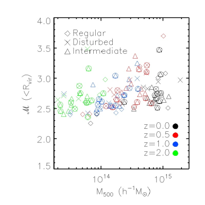
Galaxy cluster scaling relations are extremely useful to estimate cluster masses from cluster observables. In the left panel of Fig. 4 we show the mean Mach number within as a function of the cluster mass for the whole sample of 29 central clusters in the AGN simulation at redshifts and 2. The value of is shown for the populations of dynamically regular, disturbed and intermediate systems as specified in the legend. Moreover, CC clusters are marked with an additional circle around the main symbols, being all the clusters without this circle NCC clusters. Similarly, in the right panel of Fig. 4 the mean thermal energy flux, , within is shown. Table 1 shows the mean values of these quantities at for the different cluster samples. For the sake of completeness, the mean energy flux inverted in CR acceleration is also given.
On average, when all redshifts are considered, the mean Mach number value within the virial radius is almost flat as a function of cluster mass, with a significant dispersion for all redshifts (. However, if we consider the whole cluster sample at , the Pearson’s correlation coefficient between the Mach number values within the virial radius and the mass is , indicating a moderate correlation. Instead, when we consider the subsamples of regular and disturbed systems, we obtain a positive correlation with values of the Pearson’s correlation coefficient above . We have checked that this trend holds from and beyond. However, given that the considered mass range is quite narrow and the cluster sample is relatively limited, we should be cautious when deriving conclusions on this regard. As suggested by the profiles shown in Fig. 3, mild differences between dynamically regular and disturbed systems are observed throughout the radial range, contributing to a difference between the mean of regular and disturbed systems which is not found between that of CC and NCC clusters (see also Table 1).

On the contrary, as shown in the right panel of Fig. 4, the mean thermal energy flux within shows, at fixed redshift, some correlation with cluster mass although somewhat scattered. It is only combining different redshifts that a stronger correlation shows up. However, this seems to be due to the redshift dependence. Indeed, as discussed by other authors (e.g. Ryu et al., 2003), massive galaxy clusters are supposed to represent the main sites for energy dissipation at shocks. Therefore, since the total energy processed by shocks in a simulated volume depends on the number of clusters, we should be cautious when comparing these results with preceding works (e.g. Ryu et al., 2003; Pfrommer et al., 2006; Vazza et al., 2009a). According to the results shown in Table 1, at our sample of CC clusters have larger mean values of than the NCC systems. In a similar way, as for the global dynamical state of clusters, disturbed objects show larger values of the mean thermal energy flux than regular ones. Since all these cluster subsamples have similar mean virial Mach numbers, differences could be also connected with a different amount of gas density contributing to the dissipation of energy.
Therefore, according to the global analysis of Fig. 4, our results suggest that, provided that we have a significant cluster statistics, these relations could be used as potential cluster mass proxies.
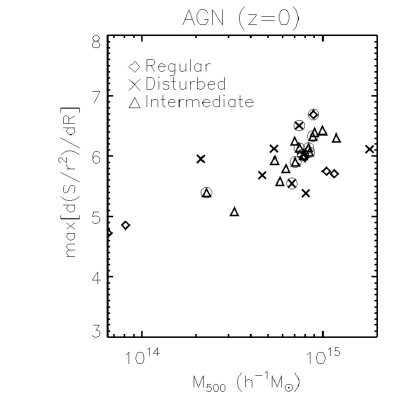
A complementary way to analyze the radial distribution of shocks around clusters is given in the left panel of Fig. 5, that shows the radial shock surface distribution, out to , for the whole sample of clusters in the AGN run at (black continuous line). This quantity provides an approximated estimation of the surface of shock cells, , at their locations, . For the sake of comparison, we also report the mean shock surface distribution obtained for the subsamples of CC/NCC and regular/disturbed systems. As shown in previous studies (Schaal and Springel, 2015; Schaal et al., 2016), this distribution provides information on the location of the main shock surfaces within and around the cluster virial region and it is, therefore, very useful to estimate the position and shape of external accretion shocks. Within the virial radius, the different mean shock surface distributions show a number of peaks or bumps which make the profiles quite irregular. These internal peaks could be connected with a number of internal shock events, such as shocks developed as a consequence of merging substructures, flow motions or feedback processes. However, above all mean profiles tend to smoothly increase out to , where the curves show their maximum value. The position of this maximum could be connected with the radius (provided that accretion shocks are assumed to be spherical) of the main external accretion shock around the central clusters. It is interesting to note that there is a clear distinction between the mean shock surface distribution associated to regular and disturbed systems, with the latter showing the highest values throughout the radial range. On the contrary, we have not found such a strong dependence of on the clusters’ core properties. Interestingly, we have obtained a moderate correlation (with a Pearson’s correlation coefficient of ) between the maximum value of the distribution and the mass of the associated systems. At , by fitting linearly the relation max (see right panel of Fig. 5), we have obtained for the whole sample of clusters in the AGN run a slope , although with some scatter444Similarly, we have obtained for the reduced sample of clusters in the CSF and NR simulations a value of and , respectively.. This trend points towards a connection between the extension (or surface filling factor) of external accretion shocks developed during the collapse of structures and the mass of the final formed systems. Assuming that future observational radio facilities, such as the Square-Kilometre Array555https://www.skatelescope.org/ (SKA; e.g. Acosta-Pulido et al., 2015), will be able to routinely detect large-scale shock waves, correlations like the one presented here, which is rather independent on the physics included, could become a complementary tool to estimate cluster masses (e.g. Planelles and Quilis, 2013).
4 Summary and Conclusions
The formation and evolution of cosmic shock waves, inherent to cosmic structure formation and evolution processes, play a main role in the energy distribution and thermalization of the IGM. In this work we have analyzed the distribution of these shocks in the Dianoga set of simulated galaxy clusters obtained from a set of zoom-in simulations performed with the SPH code GADGET-3. These simulations account for the effects of radiative cooling, star formation, SNe and AGN feedback. Previous analyses of these simulations have shown an excellent agreement with a number of observed properties of the intra-cluster medium, such as the X-ray and SZ scaling relations, the metal distribution, or the thermal and dynamical properties of CC and NCC clusters (Rasia et al., 2015; Biffi et al., 2017; Planelles et al., 2017; Biffi et al., 2018; Truong et al., 2018, 2019). We have performed a further analysis of these simulations to explore in detail the distribution and evolution of the strength of shocks as a function of cluster mass, redshift and feedback processes, paying special attention to the connection between the shock cell distribution and the cool-coreness (CC/NCC) and global dynamical state (regular/disturbed) of clusters. To perform this analysis, a grid-based shock-finding algorithm has been applied in post-processing to the outcomes of the simulations. In the following we summarize our main findings.
-
•
In general, as cluster evolution proceeds, a significant high-Mach number external accretion shock is developed around simulated clusters at . These outer accretion shocks show typically quasi-spherical shapes and are found at distances of from the cluster centre.
-
•
As already shown in previous works, most of the computational volume is filled with low-Mach number shocks (), which tend to be located within the cluster boundaries, while stronger shocks with higher Mach numbers are less numerous and tend to be found in outer cluster regions.
-
•
Low-Mach number shocks, mainly developed within collapsed and dense environments, are more relevant in thermalizing the ICM and producing CRs. As a consequence, most of the total thermal energy flux is processed by relatively low-Mach number shocks (; e.g. Vazza et al., 2011b), while stronger external shocks are energetically less important.
-
•
While the mean Mach number radial distribution within a cluster is quite flat out to (with mean values within ), the profiles raise significantly in outer cluster regions, reaching values as high as .
-
•
We do not find any relevant difference between CC and NCC clusters in terms of the shock Mach number radial distribution. However, according to the clusters’ dynamical state, disturbed systems tend to show stronger shocks than regular ones throughout the clusters’ volume.
-
•
We find that, in general, massive clusters tend to show higher mean Mach numbers within the virial radius than less massive ones and, moreover, their associated shock waves are more efficient thermalizing the IGM. This trend is even stronger when we consider the subsamples of regular and disturbed systems.
-
•
From the analysis of the shock surface distribution function we have obtained a moderate correlation between the extension of external accretion shocks developed during the collapse of structures and the mass of the final formed systems (see also Appendix B). We expect this correlation, which is independent of the physics included in the simulations, to become in principle a way to infer cluster masses.
-
•
As for the redshift evolution of the shock cell distribution we find that the fraction of cells hosting shocks in the different simulated volumes slightly increases with decreasing redshift (from per cent at out to per cent at ; see Appendix B). On the other hand, the mean Mach number remains quite flat for all clusters ().
-
•
As a consequence of the different radiative and feedback processes included in the NR, CSF and AGN simulations, some differences in the distribution of shocks within the clusters’ virial region are clearly detectable. On the contrary, the large-scale Mach number distribution, which is mainly driven by gravitational effects associated to cosmic structure formation, is very similar in the three sets of simulations (see Appendix C).
-
•
From the analysis of the shock cell distribution function around one of the most massive clusters in our sample, we find that AGN feedback tends to produce a small shortfall of shocked cells in the range , compared to the NR run. This discrepancy is similarly present when comparing the CSF and the NR simulation, suggesting its origin to be related to the impact of radiative processes in general (see Appendix C).
Although shocks can be observed at different wavelengths, such as X-rays, millimetric (via the SZ effect) and radio, their detection is challenging. However, the key role played by shocks in the thermalization and energetics of the LSS makes mandatory observing and understanding them in detail. In this regard, it is crucial to perform detailed analyses of the formation and evolution of shocks in realistic and complex simulations like the ones analyzed in this project. These studies need however to be improved in terms of shock identification and estimation of the energy dissipation at shocks. Moreover, even when the analyzed cluster sample is perfectly suitable for the present study, larger samples are needed in order to reach more robust statistical conclusions. The combination of results from simulations with the expected observations from the next generation of X-rays, SZ and radio instruments (see, for instance, Vazza et al., 2019) will be essential to deepen our understanding of the main properties of the LSS of the Universe.
ACKNOWLEDGEMENTS
We thank the anonymous referee for his/her constructive comments. This work has been performed under the Project HPC-EUROPA3 (INFRAIA-2016-1-730897), with the support of the EC Research Innovation Action under the H2020 Programme; in particular, SP gratefully acknowledges the hospitality of the Department of Physics of the University of Trieste and the computer resources and technical support provided by CINECA. SP and VQ acknowledge financial support from the Spanish Ministerio de Ciencia, Innovación y Universidades (MICINN, grant PID2019-107427GB-C33) and the Generalitat Valenciana (grant PROMETEO/2019/071). SB and ER acknowledge financial support from the PRIN-MIUR 2015W7KAWC grant and the INFN InDARK grant. VB acknowledges support by the DFG project nr. 415510302. KD acknowledges support by the Deutsche Forschungsgemeinschaft (DFG, German Research Foundation) under Germany’s Excellence Strategy - EXC-2094 - 3907833 as well as the COMPLEX project from the European Research Council (ERC) under the European Union’s Horizon 2020 research and innovation program grant agreement ERC-2019-AdG 860744.
Data availability
The data underlying this article will be shared on reasonable request to the corresponding author.
References
- Acosta-Pulido et al. (2015) Acosta-Pulido J.A., et al., 2015, ArXiv e-prints
- Axford et al. (1977) Axford W.I., Leer E., Skadron G., 1977, International Cosmic Ray Conference, 11, 132
- Bassini et al. (2020) Bassini L., et al., 2020, arXiv e-prints, arXiv:2006.13951
- Beck et al. (2016a) Beck A.M., Dolag K., Donnert J.M.F., 2016a, MNRAS, 458, 2080
- Beck et al. (2016b) Beck A.M., et al., 2016b, MNRAS, 455, 2110
- Biffi et al. (2018) Biffi V., Planelles S., Borgani S., Rasia E., Murante G., Fabjan D., Gaspari M., 2018, ArXiv e-prints
- Biffi et al. (2016) Biffi V., et al., 2016, ApJ, 827, 112
- Biffi et al. (2017) Biffi V., et al., 2017, MNRAS, 468, 531
- Blandford and Ostriker (1978) Blandford R.D., Ostriker J.P., 1978, ApJ, 221, L29
- Blasi (2007) Blasi P., 2007, Nuclear Physics B Proceedings Supplements, 165, 122
- Bonafede et al. (2011) Bonafede A., Dolag K., Stasyszyn F., Murante G., Borgani S., 2011, MNRAS, 418, 2234
- Brüggen et al. (2012) Brüggen M., Bykov A., Ryu D., Röttgering H., 2012, Space Sci. Rev., 166, 187
- Brunetti and Jones (2014) Brunetti G., Jones T.W., 2014, International Journal of Modern Physics D, 23, 1430007-98
- Bryan and Norman (1998) Bryan G.L., Norman M.L., 1998, ApJ, 495, 80
- Bykov et al. (2008) Bykov A.M., Dolag K., Durret F., 2008, Space Sci. Rev., 134, 119
- Dasadia et al. (2016) Dasadia S., et al., 2016, ApJ, 820, L20
- De Luca et al. (2021) De Luca F., De Petris M., Yepes G., Cui W., Knebe A., Rasia E., 2021, MNRAS, 504, 5383
- Dolag et al. (2008) Dolag K., Bykov A.M., Diaferio A., 2008, Space Sci. Rev., 134, 311
- Erler et al. (2015) Erler J., Basu K., Trasatti M., Klein U., Bertoldi F., 2015, MNRAS, 447, 2497
- Ferrari et al. (2008) Ferrari C., Govoni F., Schindler S., Bykov A.M., Rephaeli Y., 2008, Space Sci. Rev., 134, 93
- Ha et al. (2018) Ha J.H., Ryu D., Kang H., 2018, ApJ, 857, 26
- Hoeft et al. (2008) Hoeft M., Brüggen M., Yepes G., Gottlöber S., Schwope A., 2008, MNRAS, 391, 1511
- Hong et al. (2014) Hong S.E., Ryu D., Kang H., Cen R., 2014, ApJ, 785, 133
- Hong et al. (2015) Hong S.E., Kang H., Ryu D., 2015, ApJ, 812, 49
- Kang et al. (2007) Kang H., Ryu D., Cen R., Ostriker J.P., 2007, ApJ, 669, 729
- Landau and Lifshitz (1966) Landau L.D., Lifshitz E.M., 1966, Hydrodynamik
- Markevitch et al. (2002) Markevitch M., Gonzalez A.H., David L., Vikhlinin A., Murray S., Forman W., Jones C., Tucker W., 2002, ApJ, 567, L27
- Markevitch et al. (2005) Markevitch M., Govoni F., Brunetti G., Jerius D., 2005, ApJ, 627, 733
- Martin-Alvarez et al. (2017) Martin-Alvarez S., Planelles S., Quilis V., 2017, Ap&SS, 362, 91
- Miniati et al. (2000) Miniati F., Ryu D., Kang H., Jones T.W., Cen R., Ostriker J.P., 2000, ApJ, 542, 608
- Miniati et al. (2001) Miniati F., Jones T.W., Kang H., Ryu D., 2001, ApJ, 562, 233
- Nelson et al. (2016) Nelson D., Genel S., Pillepich A., Vogelsberger M., Springel V., Hernquist L., 2016, MNRAS, 460, 2881
- Pfrommer et al. (2006) Pfrommer C., Springel V., Enßlin T.A., Jubelgas M., 2006, MNRAS, 367, 113
- Pfrommer et al. (2007) Pfrommer C., Enßlin T.A., Springel V., Jubelgas M., Dolag K., 2007, MNRAS, 378, 385
- Pfrommer et al. (2008) Pfrommer C., Enßlin T.A., Springel V., 2008, MNRAS, 385, 1211
- Planck Collaboration et al. (2013) Planck Collaboration, et al., 2013, A&A, 554, A140
- Planelles and Quilis (2013) Planelles S., Quilis V., 2013, MNRAS, 428, 1643
- Planelles et al. (2013) Planelles S., Borgani S., Dolag K., Ettori S., Fabjan D., Murante G., Tornatore L., 2013, MNRAS, 431, 1487
- Planelles et al. (2014) Planelles S., Borgani S., Fabjan D., Killedar M., Murante G., Granato G.L., Ragone-Figueroa C., Dolag K., 2014, MNRAS, 438, 195
- Planelles et al. (2015) Planelles S., Schleicher D.R.G., Bykov A.M., 2015, Space Sci. Rev., 188, 93
- Planelles et al. (2017) Planelles S., et al., 2017, MNRAS, 467, 3827
- Quilis et al. (1998) Quilis V., M J., Ibáñez ., Sáez D., 1998, ApJ, 502, 518
- Ragone-Figueroa et al. (2018) Ragone-Figueroa C., Granato G.L., Ferraro M.E., Murante G., Biffi V., Borgani S., Planelles S., Rasia E., 2018, MNRAS, 479, 1125
- Rasia et al. (2015) Rasia E., et al., 2015, ApJ, 813, L17
- Rephaeli et al. (2008) Rephaeli Y., Nevalainen J., Ohashi T., Bykov A.M., 2008, Space Sci. Rev., 134, 71
- Röttgers and Arth (2018) Röttgers B., Arth A., 2018, arXiv e-prints, arXiv:1803.03652
- Ryu et al. (2003) Ryu D., Kang H., Hallman E., Jones T.W., 2003, ApJ, 593, 599
- Schaal and Springel (2015) Schaal K., Springel V., 2015, MNRAS, 446, 3992
- Schaal et al. (2016) Schaal K., et al., 2016, MNRAS, 461, 4441
- Skillman et al. (2008) Skillman S.W., O’Shea B.W., Hallman E.J., Burns J.O., Norman M.L., 2008, ApJ, 689, 1063
- Springel (2005) Springel V., 2005, MNRAS, 364, 1105
- Steinborn et al. (2015) Steinborn L.K., Dolag K., Hirschmann M., Prieto M.A., Remus R.S., 2015, MNRAS, 448, 1504
- Sunyaev and Zel’dovich (1980) Sunyaev R.A., Zel’dovich I.B., 1980, MNRAS, 190, 413
- Truong et al. (2018) Truong N., et al., 2018, MNRAS, 474, 4089
- Truong et al. (2019) Truong N., et al., 2019, MNRAS, 484, 2896
- Vazza et al. (2009a) Vazza F., Brunetti G., Gheller C., 2009a, MNRAS, 395, 1333
- Vazza et al. (2009b) Vazza F., Brunetti G., Kritsuk A., Wagner R., Gheller C., Norman M., 2009b, A&A, 504, 33
- Vazza et al. (2010) Vazza F., Brunetti G., Gheller C., Brunino R., 2010, New Astron., 15, 695
- Vazza et al. (2011a) Vazza F., Brunetti G., Gheller C., Brunino R., Brüggen M., 2011a, A&A, 529, A17
- Vazza et al. (2011b) Vazza F., Dolag K., Ryu D., Brunetti G., Gheller C., Kang H., Pfrommer C., 2011b, MNRAS, 418, 960
- Vazza et al. (2012) Vazza F., Roediger E., Brüggen M., 2012, A&A, 544, A103
- Vazza et al. (2013) Vazza F., Brüggen M., Gheller C., 2013, MNRAS, 428, 2366
- Vazza et al. (2014) Vazza F., Gheller C., Brüggen M., 2014, MNRAS, 439, 2662
- Vazza et al. (2016) Vazza F., Brüggen M., Wittor D., Gheller C., Eckert D., Stubbe M., 2016, MNRAS, 459, 70
- Vazza et al. (2019) Vazza F., Ettori S., Roncarelli M., Angelinelli M., Brüggen M., Gheller C., 2019, A&A, 627, A5
- Villaescusa-Navarro et al. (2016) Villaescusa-Navarro F., et al., 2016, MNRAS, 456, 3553
- Zhang et al. (2020) Zhang C., Churazov E., Dolag K., Forman W.R., Zhuravleva I., 2020, MNRAS, 494, 4539
Appendix A Dependence on grid resolution


When we smooth a distribution of SPH particles onto a grid, ideally, we want to reach a grid resolution comparable with the resolution we have in the SPH simulation. However, this is not trivial, especially when we employ a regular grid (see Röttgers and Arth, 2018, for a recent analysis of different smoothing methods). Therefore, once we have smoothed a distribution of particles onto a grid, we need to make sure that, for instance, the total mass inside the considered volume is conserved. This means that we should get the same gas mass within a given region when comparing the summation over all SPH particles with the integral of the gas density over a grid. To address this issue, Fig. 6 shows the mean relative error in recovering the gas mass within different radial apertures from the cluster centre as obtained for the whole sample of 29 clusters in the AGN simulations at . The considered apertures are spherical regions of radius equal to and 4 times the virial radius of each halo. The last tick mark on the x-axis, labelled as ‘Box’, stands for the volume of the whole cubical box, that is, including as well the corners of the box and not just the sphere, with side length equal to . Then, the error in mass is computed as the relative difference between the mass obtained from the direct summation over the sample of particles within a given region and from the integration of the gas density smoothed out onto a grid of a given resolution, that is, , being and the masses derived from the distribution of particles and from the grid. Results are shown for three different resolutions which correspond to discretize the considered volumes with , and cells (black, green and red lines, respectively). The results shown in this figure indicate that when we consider the lowest resolution, the one corresponding to cells, the error in mass is around 1 per cent for all the considered radial apertures. Instead, when we increase the grid resolution the error increases significantly, especially for the resolution corresponding to cells and for radial apertures beyond .
To understand better this trend, Fig. 7 shows the distribution of the mean smoothing length of all the gas particles within different radial apertures from the cluster centre for each of the 29 main halos in the AGN simulations at (black continuous lines). As expected, the mean smoothing length of particles within clusters is relatively low within the virial radius (kpc) and increases in outer regions (kpc). As in the previous figure, we have considered spherical regions of radius equal to and 4 times the virial radius of each halo. We have also considered the volume of the whole cubical box with side length equal to . Horizontal lines represent the corresponding mean grid resolutions when discretizing the considered volumes with , and cells (horizontal black, green and red lines, respectively). An additional horizontal blue line represents the mean smoothing length of all gas particles as obtained from the whole sample of 29 clusters. According to these results, the resolution corresponding to a grid with cells (horizontal black line) is comparable to the mean smoothing length of all particles (kpc; horizontal blue line). Although this is a simple approximation, in view of the results shown in Figs. 6 and 7, we decided to adopt as our reference resolution the one corresponding to discretize the distribution of particles onto a regular grid with cubical cells.
Early studies with grid-based cosmological codes (e.g. Kang et al., 2007) have shown that for a fixed grid resolution it is difficult to capture smaller-scale shock features, meaning that shocks in inner cluster regions may not be fully identified. In our study we have checked that, as the spatial grid resolution is artificially increased, a larger amount of weaker and thinner shock surfaces can be identified. We should, however, take this result with caution since, as shown for the mass conservation in Fig. 6, the artificial improvement of the grid resolution can generate unrealistic and spurious identification of shocks. Therefore, trying to resolve shocks in cluster outskirts with a grid resolution higher than the actual SPH resolution may introduce significant spurious effects. Indeed, the proper way to study the effect of spatial resolution on our results would be to re-simulate the sample of 29 regions, with the same initial conditions, but with different mass resolutions. Although this option is beyond the purpose of this paper, it could be addressed in future works. Therefore, taking into account the results discussed in this section, we have chosen the resolution corresponding to cells as our reference one throughout the paper.
Appendix B Connection between shocks and galaxy clusters
| cluster | core | dynamical | ||||||
|---|---|---|---|---|---|---|---|---|
| [] | [] | [] | state | state | [] | [] | [] | |
| D2 | 5.26 | 1.70 | 0.74 | CC | Intermediate | 105.3 | 52.9 | 26.5 |
| D3 | 6.53 | 1.83 | 0.84 | NCC | Intermediate | 113.3 | 56.9 | 28.5 |
| D4 | 5.21 | 1.69 | 0.73 | NCC | Disturbed | 105.0 | 52.7 | 26.4 |
| D6 | 15.41 | 2.43 | 1.08 | NCC | Intermediate | 150.8 | 75.7 | 37.9 |
| D10 | 15.46 | 2.43 | 1.07 | CC | Disturbed | 151.1 | 75.9 | 38.0 |
| D21 | 14.26 | 2.37 | 1.17 | CC | Regular | 146.9 | 73.8 | 37.0 |
In order to analyze in more detail the connection between the distribution of shock waves and the dynamical or cool-coreness state of the clusters, in this Section we will focus our analysis on a smaller selection of 6 systems, whose main properties are summarized in Table 2. Although this reduced sample is not statistically representative, it has been chosen in order to have systems with different masses, core and dynamical classifications.


Figure 8 shows projections along the z-axis of the gas overdensity and the Mach number distribution around each of the 6 selected cluster regions at (including region D21, whose redshift evolution has been shown in Fig. 1). For the central cluster of each region, radii , , and are also shown. According to the density maps, these projections clearly show a wide variety of large-scale structures around the different haloes. Indeed, outside the virial radius, a complex and irregular distribution of filaments and void regions dominate the simulated volume. As expected, within the clusters’ virial region the density distribution is dominated by the very central area within , although smaller substructures are also visible in outer regions, in-between and .
Interestingly, if we look instead at the shock Mach number maps shown in Fig. 8, most of the regions show a high-Mach number shock surface (located at several virial radii from the cluster centre) wrapping the large scale density distribution and separating the external unshocked gas from the cluster outskirts. Although the shape of these external accretion shocks is assumed to be quasi-spherical, as in region , there are some other regions, like , or , which show a more irregular “flower-like” distribution. Some studies have shown that this particular pattern is quite common and results from the intersection between merger and accretion shocks developed during clusters’ evolution (e.g. Zhang et al., 2020). Instead, within the virial radius clusters show different and more irregular shock patterns. In some regions, like or , some bow shocks with low Mach number are detectable in the area within and .
Similarly to Fig. 2, we show in Fig. 9 the shock cell distribution function (left panel) and the differential distribution of the thermal energy flux through shocks (right panel) for the reduced sample of clusters in the AGN simulation at . These distributions have been computed for a cubical region of side length equal to around each cluster. Obviously, for all clusters both distributions show a broad agreement with the mean trend shown in Section 3.1 for the complete sample of systems. In general, we do not distinguish any particular trend depending on the core or global dynamical state of the different clusters. However, for a fixed Mach number, the most massive clusters (i.e. D6, D10 and D21) tend to host a larger percentage of shocked cells and seem to be more efficient in thermalizing the IGM, in agreement with the results shown in Fig. 4. In addition, even though regions D6, D10 and D21 are quite similar in terms of the shock cell distribution function through most of the Mach number range, shocks within region D21 (connected to the only dynamically regular system in our sample) seem to process a lower amount of energy than shocks within regions D6 and D10, especially for . A similar trend was also obtained by Vazza et al. (2010), who found mild differences, especially for shocks with , between their merging and relaxed cluster samples, with the relaxed systems processing times less thermal energy than the merging ones.
It is also important to stress that the distributions shown in Figs. 2 and 9 are derived from the 3D distribution of shocks around each cluster, while the maps are projections of a slice across the cluster centre. In this way, most of the shocks that boost the SDF at high Mach number for region D6 are not visible from the map.
The left panel of Fig. 10 reports the mean Mach number radial profiles, out to , for the reduced sample of clusters at . Despite the different dynamical classification of the systems, they show very similar radial Mach number distributions, especially within . Indeed, out to the viral radius, all clusters show mean Mach number values within . Above the mean strength of shocks smoothly increases, reaching values as high as at . As discussed in Section 3.1, the shape of these profiles is in line with the results presented in previous analyses (e.g. Vazza et al., 2009a, 2010, 2011b). In our case, we do not find either a clear trend depending on the dynamical state of the clusters nor on their cool-coreness. In this regard, it is interesting to remind that the classification in relaxed/disturbed systems was done within and, therefore, it does not mean that a relaxed cluster must have a smooth gas density distribution up to . However, we still note that at the shock cell distributions within regions D6, D10 and D21 reach higher Mach numbers than shocks within the rest of regions.
In order to explore the global efficiency of these systems in accelerating CR at shocks, the right panel of Fig. 10 shows the mean radial profiles of the ratio between the CR energy flux and the thermal energy flux, , at . On average, regardless of the dynamical state of the different clusters, we do not find relevant differences between them throughout the radial range. However, region D21 shows larger values than expected, especially below . These peaks in the radial distribution must be connected with the slightly larger radial Mach number profiles shown by this system in the central regions (see left panel). Leaving aside these deviations, the mean radial distribution of the ratio tends to increase with the distance from the cluster centre, providing stringent limits to the energy dissipation ratio. Although it is not possible to perform a straightforward comparison among different simulations, the obtained trend and average value of the ratio is in line with the estimates shown in previous works (see, e.g., Vazza et al., 2009a, where some dependences of the ratio on the energy dissipation model employed are also shown).
As it has been shown in Fig. 5, Fig. 11 shows now the radial shock surface distribution, out to , for the reduced sample of clusters in the AGN run at . Since this distribution gives an idea of the location of the main shock features within and around the cluster virial region, it can be correlated with the maps of the shock Mach number distribution shown in Fig. 8. For each halo the bumps characterising the distribution within highlight the presence of internal shock phenomena. Outside the virial radius, most clusters show a dominant peak in the radial shock surface distribution, which approximately indicates the position of the main external accretion shock. The distributions, however, show quite irregular shapes that depend on the particular clusters’ environments and evolutionary histories. Although usually it is not possible to clearly distinguish the radius for the accretion shock (see, for instance, region D3), on average, we find the external accretion shock at a mean distance of from the cluster centre, a value a bit larger than the results presented in previous studies (e.g. Schaal and Springel, 2015; Schaal et al., 2016; Nelson et al., 2016). As discussed in Section 3.1, the height of the external peaks in the radial shock surface distribution shows some dependence on cluster mass. In this case, leaving aside some unavoidable deviations resulting from the particular clusters’ evolution, the height of the distributions is clearly larger in two of the most massive systems in our sample, i.e., and . As for region , although the peak of the distribution is similar to that of the smallest systems, it starts from below and, therefore, its absolute increase is also remarkably higher than for regions , or . This result is in line with the fact that, in general, the extension of accretion shocks is larger around the most massive clusters (e.g. Miniati et al., 2000).
We now investigate the temporal evolution of different global shock-related quantities for the reduced sample of clusters. Figure 12 shows the redshift evolution of the fraction of the computational volume hosting shocked cells (left panel), the mean Mach number of all the cells hosting shocks (middle panel), and the ratio of CR energy flux over the thermal energy flux through shocked cells in each computational volume (right panel). All these quantities have been computed within a box of side length equal to of the main cluster of each selected region. From the analysis of this figure we obtain several interesting conclusions. The fraction of cells hosting shocks in the different simulated volumes slightly increases from an average value of per cent at up to a value of per cent at . The mean values obtained at are larger than those reported in previous studies (%, e.g. Vazza et al., 2009a; Planelles and Quilis, 2013). However, we should keep in mind that, in comparison with a cosmological volume, we are analysing a smaller and, therefore, a denser region around large clusters, which contributes to augment the amount of shocked cells. The mild increasing trend with decreasing redshift is in line with the results shown in Figs. 1 and 2 for the complete sample of clusters as well as with the results shown in other analyses (e.g. Vazza et al., 2009a). As for the z-evolution of the mean Mach number, the mean strength of shocks shows values within for all clusters. In most of the regions the average Mach number tends to be slightly larger at than at . In this regard, region , whose main central cluster was classified as a dynamically relaxed system, shows the lowest global variation between the high-z and the final Mach number values. According to the z-evolution of the ratio, leaving aside some particular deviations, the mean amount of energy allocated for CR acceleration seems to be larger at higher redshift and to slightly decrease with time. In all regions, on average, the ratio of the CR over the thermal energy flux is around . At the present epoch we find a value of within , in line with the values obtained in previous analyses (e.g. within in Vazza et al., 2009a, depending on the adopted model of energy dissipation and on the considered environment). Although the approximation employed to estimate in post-processing is reasonable, we should keep in mind that this is a simplified treatment of the energy dissipation at shocks. Indeed, the fact that shows larger values at early cosmic epochs claims for the need to properly, and self-consistently, solve the dynamics of the CR population and to account for its effects on the thermal distribution of the IGM (e.g. Pfrommer et al., 2006, 2007, 2008; Vazza et al., 2016). This analysis is however beyond the scope of the present work.
Appendix C Dependence on baryonic physics


In this Appendix we explore the effect of different prescriptions for the physics of baryons on the shock cell distribution. In particular, we compare the distribution of Mach numbers at for the region associated to the most massive cluster in our sample, i.e., region D21, as obtained from the NR, CSF and AGN simulations.
Figures 13 and 14 show, respectively, 2-D zoom projections of the gas overdensity and the Mach number distribution within the whole considered volume and within the virial radius of cluster D21 in the NR, CSF and AGN simulations at . Independently of the considered region, although the density distributions of all three runs are quite similar, both radiative runs show a larger number of small density peaks which are mainly associated to radiative cooling and star formation processes. However, the action of AGN feedback dilutes some of these clumps and generates a much puffier density distribution than in the CSF run (see also Planelles et al., 2014). This effect if more clearly distinguishable in the upper panel of Fig. 14.
As already anticipated in Section 3.1, Fig. 13 shows that the large-scale shock cell distribution obtained for region D21 is very similar in all three runs. This behaviour was expected, since shocks in cluster outskirts are mainly driven by gravitational effects associated to cosmic structure formation processes. However, as shown in the lower panels of Fig. 14, some differences in the distribution of shocks obtained in the NR, CSF and AGN simulations are detectable within the cluster virial region (e.g. Vazza et al., 2013; Schaal et al., 2016). Although in this particular case these differences are relatively minor, they result from the different radiative and feedback processes included in our simulations. This behavior is also displayed in the Mach number radial profiles shown in the left panel of Fig. 15.
For the sake of completeness, the right panel of Fig. 15 shows the shock cell distribution function within a volume of side length equal around the centre of cluster D21 as obtained in the NR, CSF and AGN simulations at . As already discussed in previous studies (e.g. Vazza et al., 2013), we find a small shortage of shocks in the AGN simulation, especially within . This difference is particularly significant between the AGN and the NR simulations: on average, AGN feedback tends to increase the mean ICM temperature, thus affecting the sound speed in the medium and, therefore, decreasing the corresponding strength of shocks. This discrepancy is similarly present when comparing the CSF and the NR simulations. Overall, these results suggest that the inclusion of radiative cooling, which removes some gas from the diffuse accretion, plays the main role, while the effect of changing the feedback prescription, namely including or not AGN feedback, is rather minor.