Exploring blazars through
sonification.
Visual and auditory insights into multifrequency variability
Abstract
Using open astronomical multifrequency databases, we constructed light curves and developed a comprehensive visualisation and sonification analysis for the blazars Mrk 501, Mrk 1501, Mrk 421, BL Lacerta, AO 0235+164, 3C 66A, OJ 049, OJ 287, and PKS J2134-0153. This study employed Musical Instrument Digital Interface (MIDI) and Parameter Mapping Sonification (PMSon) techniques to generate waveforms, spectrograms, and sonifications. These representations demonstrate that data visualisation and sonification are powerful tools for analysing astronomical objects like blazers, providing insights into their multifrequency variability. This work highlights how sonification and visualisation can aid in identifying potential patterns, power variations, regularities, and gaps in the data. This multimodal approach also underscores the importance of inclusivity in scientific communication, offering accessible methods for exploring the complex behaviour of blazers.
keywords:
astronomical data bases: miscellaneous, virtual observatory tools, software: data analysis1 Introduction
Data visualisation, often referred to as DataViz, serves as a valuable approach for identifying and discerning patterns or recurring trends within the behaviours of social or natural phenomena. It leverages its cognitive and explanatory capabilities through techniques such as time series, histograms, infographics, and Venn-Euler diagrams (Friendly, 2008). Consequently, graphical representation stands as a fundamental method for conducting research in the realms of science and study.
DataViz stands as a important methodology for both scientific communication and research. Nonetheless, it is essential to consider a couple of factors. Firstly, it is important to recognise that visual communication is not accessible to individuals who are blind or have visual impairments (BVI) (Pérez-Montero, 2019). Secondly, relying solely on graphical representations might prove insufficient when dealing with comprehensive data analysis. Therefore, incorporating supplementary review methods becomes indispensable to enhance the research process.
Taking this into account, data sonification can serve not only as a means of inclusivity in scientific communication but also as an additional tool for research (Sawe et al., 2020). By transforming data into sound, it offers an alternative mode of perception that complements visual representations, allowing for a deeper understanding of complex data.
As Kramer et al. (1999) defines it, data sonification as “the transformation of data relations into perceived relations in an acoustic signal for the purposes of facilitating communication or interpretation” highlights sonification as a valuable supplementary instrument for comprehending information. Unlike the sense of vision, hearing excels in perceiving information over time, as well as recognising patterns and momentary fluctuations. Therefore, sonification proves to be an excellent aid in enhancing knowledge understanding (Guttman et al., 2005).
Another definition of data sonification, provided by Hermann (2008), characterises it as a technique that takes data as its input and produces sound signals, possibly in response to optional additional stimulation or triggering. This broad definition encompasses any process that uses data to create auditory outputs and can be referred to as sonification, if and only if the following conditions are satisfied:
-
•
The sound reflects objective properties or relations of the input data.
-
•
The transformation is systematic. This means that there is a precise definition provided of how the data (and optional interactions) cause the sound to change.
-
•
The sonification is reproducible: given the same data and identical interactions (or triggers), the resulting sound has to be structurally identical.
-
•
The system can intentionally be used with different data and also be used in repetition with the same data.
Following Hermann (2008) and Vogt (2008), the “sonification is the data-dependent generation of sound, if the transformation is systematic, objective and reproducible, so that it can be used as scientific method.”
Numerous instances demonstrate the effectiveness of data sonification as a valuable science communication tool. Notable examples include its application in depicting salmon migration patterns (Hegg et al., 2018) and visualising fluctuations in brainwave activity (Parvizi et al., 2018). The Geiger counter represents yet another compelling case in point.
In the realm of astronomy, early instances of data sonification trace to Jansky (1933), when detected radio waves emanating from the centre of the Milky Way were analysed by telephone communication noise. Three decades later, Penzias & Wilson (1965) identified the interference in their observations as originating from cosmic microwave background radiation, marking a significant discovery in the field (Kellermann et al., 2020).
Another example is that of Morgan et al. (1997) who took the data of the X-ray emission of the black hole GRS 1915+105 and translated it into audio signals, allowing us to “hear” the accretion disk from it Masetti (2013). Also Chandra (2003) has sonified data and released “Hears” of a black hole for the first time.
Abbott et al. (2016) documented the simultaneous detection of a brief signal by two gravitational wave detectors, which resulted from the fusion of two black holes. The researchers converted the data from the instant of the collision, which they dubbed a “chirp.” This term was chosen because certain events producing gravitational waves exhibit auditory similarities to the chirping sounds of birds (LIG, , see https://youtu.be/QyDcTbR-kEA).
Furthermore, Berti (2016) published an article entitled The First Sounds of Merging Black Holes, shedding light on the initial auditory cues of black hole mergers. In recent times, the National Aeronautics and Space Administration (NASA) has unveiled sonification imagery derived from optical data captured by the Hubble Space Telescope (NASA, 2022) and X-ray data observed by the Chandra X-ray Observatory (CXO) (Chandra, 2020).
In the context of communicating science to the BVI community, especially in the realm of astrophysics and black holes (BHs) this work sonifies data from nine blazars: Mrk 501, Mrk 1501, Mrk 421, BL Lacerta, AO 0235+164, 3C 66A (PKS 0219+428), OJ 049 (PKS 0829+046), OJ 287, and PKS J2134-0153.
Blazars are extragalactic sources of luminosity with energy outputs ranging from (Blandford et al., 2019), and their emission jets align with the observer’s line of sight (Ulrich et al., 1997). These celestial objects emit varying forms of non-thermal radiation across the entire electromagnetic (EM) spectrum (Padovani et al., 2012).
2 Obtaining the data
2.1 Radio
The radio datasets for this work were obtained from three data bases: the Owens Valley Radio Observatory (OVRO)111https://sites.astro.caltech.edu/ovroblazars/, the University of Michigan Radio Astronomy Observatory (UMRAO)222https://dept.astro.lsa.umich.edu/datasets/umrao.php, and the Astrogeo Very-long-baseline interferometry (Astrogeo-VLBI).
OVRO has been monitoring blazars searching quasi-periodic oscillations and correlations between radio and -rays in blazars (Abdo et al., 2009; Abdo et al., 2011b) since 2008 (Richards et al., 2011). It is a telescope with a cryogenic receiver at a central frequency, a bandwidth and two symmetric off-axis beams.
The 26-meter paraboloid UMRAO monitoring in the bands: 4.8, 8, and 14.5 GHz (Aller et al., 1985). It is focused on the study of total flux density and linear polarisation of active extragalactic objects333https://lsa.umich.edu/astro/facilities/data-sets.html.
Radio Fundamental Catalog (RFC), of the Astro-geo Center, maintained by L. Petrov444 http://astrogeo.org/rfc provides precise positions with milli-arcseconds accuracies, maps, and estimates of correlated flux densities at baselines 1000–8000 km of thousands of compact radio sources.
2.2 Optical
For optical, the databases used were: American Association of Variable Star Observers (AAVSO)555https://www.aavso.org/ and Zwicky Transient Facility (ZTF)666https://www.ztf.caltech.edu/.
The optical AAVSO is a public database founded in 1910 and offers observations of variable stars collected and archived for world-wide access in collaboration with amateur and professional astronomers. It is an international organisation of long-term variable star observers who participate in scientific discovery through variable star astronomy.
The ZTF is a robotic time-domain survey with a 47 square degree field with a 600 megapixel camera to scan the entire northern visible sky at rates of 3760 square degrees/hour to median depths of g 20.8 and r 20.6 mag (AB, 5 in 30 sec). ZTF has been studied in the temporal and dynamic sky as near-Earth asteroids, fast-evolving flux transients, and of Galactic variable sources (e.g. Graham et al., 2019).
2.3 X-rays
For the X-rays light curve, we use the Swift database with energies in the range . It contains the X-Ray Telescope (XRT) with two important characteristics that makes it important for observations: low background and a constant point spread function across the field of view (Moretti et al., 2005).
2.4 Gamma-rays
The public database of -rays used was of The Fermi Large Area Telescope (LAT). This instrument observes the sky for 3 hours and covers 20% of it for each observation. It has a crystal calorimeter for energy measurement, an anti-coincidence detector to distinguish the background of charged particles and high-resolution converter tracker for direction measurement of the incident gamma rays (Atwood et al., 2009). The -rays fluxes collected are in the range .
3 Sonification
Sonifying the data for each of the blazar frequencies was carried out in three stages: pre-production, production and post-production.
3.1 Pre-production
Sonification pre-production basically focuses on data pre-processing. In the case of the radio and optical bands, the data was processed in such a way that any anomaly, disturbance or irrelevance of the data could be detected, eliminated, corrected or transformed. For this task the AWK pattern scanning and processing language was used.
In the case of X-rays, it was necessary to reduce the data and for this, the HEASoft777https://heasarc.gsfc.nasa.gov/docs/software/lheasoft/ software was used. The data processing corresponding to the photons, the position and the orientation of the satellite is available on Flexible Image Transport System format files (FITS).
For the pre-production of sonification in the -rays, the data reduction was possible with the Fermitools888https://fermi.gsfc.nasa.gov/ssc/data/analysis/software/ software. For this, it was necessary to know the main relevant parameters of the blazars such as: R.A., Dec., Region of Interest (ROI) and start and end time of the data processing (see e.g Magallanes-Guijón, 2020). The process of this reduction followed the procedure detailed by Cabrera et al. (2013).
Finally, with all datasets multiwavelength light curves with discrete data of time measured in Modified Julian Days (MJD), luminosity and its uncertainty at a 3 confidence level, were produced.
3.1.1 Light curves
Each blazar selected had the following specifications:
(1) Mrk 501, has a redshift = 0.034 that corresponds to a distance 140 Mpc and R. A. = 16h 53m 52.2s, Dec. = +39° 45’ 37”. It has been monitored in radio (Richards et al., 2011), optical (Smith et al., 2009), X-rays (Abdo et al., 2011a), and -rays (Dorner et al., 2017). This object has several periodicities reported (Bhatta, 2019). Recently Magallanes-Guijón & Mendoza (2022) have reported a periodicity 224 days.
The radio dataset for Mrk 501 is from 2009 January 22 to 2020 June 27 and was obtained from the OVRO database. The light curve in optical was built using the database from 1998 June 24 to 2021 September 12. The Swift database is from 2008 October 2 to 2021 October 8. And the -rays, covers a time interval from 2008 August 04 up to 2020 March 13. Table 1 shows specific information about the records and the light curve is presented in Figure 1.
| Band | Records | Interim | Total |
|---|---|---|---|
| [y, m, d] | [d] | ||
| Radio | |||
| Optical | |||
| X-rays | |||
| -rays |


.
(2) Mrk 1501 is a FSRQ with redshift of = 0.089338 at a distance of 377 Mpc (Sargent & Searle, 1970). This blazar presents short-lived -ray emission flares Arsioli & Polenta (2018). It is in the Pisces’s constellation, with R. A. = 00h 10m, and Dec. = +10° 58’. (Markarian et al., 1989).
The radio dataset for Mrk 1501 was obtained from OVRO, from 2008 May 1 to 2020 June 30. For the optical, the dataset was taken from the ZTF database, from 2010 July 25 to 2021 November 25. In the case of X-rays the database comes from the Swift observatory from 2008 October 2 to 2021 March 22. For the period of 2008 August 4 to 2022 October 22, the dataset is from the Fermi database. Table 2 shows the summary of the dataset, and Figure 2 presents the light curves.
| Band | Records | Interim | Total |
|---|---|---|---|
| [y, m, d] | [d] | ||
| Radio | |||
| Optical | |||
| X-rays | |||
| -rays |


.
(3) BL Lacerta was discovered in 1929 by Hoffmeister (1929) and Oke & Gunn (1974) measured its redshift = 0.07 which corresponds to a distance of 0.276 Gpc. It is in the constellation Lacertae, with R. A. = 22h 02m 43.3s, Dec. = +42° 16’ 40” (Miller et al., 1978).
The dataset in radio for this object was obtained from UMRAO from 2009 September 1 to 2012 May 21. For optical, the dataset used was from AAVSO in an interim of 1969 December 14 to 2022 March 13. For X-rays, the time interval is 2008 October 2 to 2022 November 10, taken from the Swift Observatory. And for -rays, the time of observation was from 2008 August 4 to 2022 March 11. Table 3 presents the summaries of the dataset and the light curves are shown in Figure 3.
| Band | Records | Interim | Total |
|---|---|---|---|
| [y, m, d] | [d] | ||
| Radio | |||
| Optical | |||
| X-rays | |||
| -rays |


.
(4) AO 0235+164 is a BL Lac object999D’Elia et al. (2015) suggest that it could classify as an FSRQ according to its strong H feature in the IR band. with a R. A. = 02h 35m 52.6s, Dec. = 16° 24’ 05”. (Spinrad & Smith, 1975) and redshift of = 0.940 corresponding to a distance of 3 Gpc Cohen et al. (1987).
For AO 0235+164, the radio dataset was obtained from OVRO from 2008 January 6 to 2020 June 24. For optical, the time period was from 1998 August 25 to 2020 September 13, and the database used was from AAVSO. For X-rays, the dataset used was from Swift from 2008 October 2 to 2017 December 7. The Fermi -rays database was taken from 2008 August 4 to 2020 April 5. Table 4 shows a summary of these details and Figure 4 presents the corresponding light curves.
| Band | Records | Interim | Total |
|---|---|---|---|
| [y, m, d] | [d] | ||
| Radio | |||
| Optical | |||
| X-rays | |||
| -rays |


.
(5) 3C 66A has a redshift of = 0.34 corresponding to 1.4 Gpc (Torres-Zafra et al., 2018). This BL Lac object has been observed on optical wavelengths (e. g. Böttcher et al., 2005; Lainela et al., 1999). It has R.A. = 2h 23m 12s and Dec.= 43° 0.’7 reported by Errando et al. (2009) in -rays.
The records from the Astro-geo VLBI were taken from 1997 January 11 to 2020 June 4. For optical, the dataset used was from AAVO from 1994 February 1 to 2022 February 10. The Swift X-rays database used is from 2008 October 2 to 2022 December 9. All these specifications are presented in Table 5 and the light curves are shown in Figure 5.
| Band | Records | Interim | Total |
|---|---|---|---|
| [y, m, d] | [d] | ||
| Radio | |||
| Optical | |||
| X-rays | |||
| -rays |


.
(6) OJ 049 has a redshift = 0.18 , corresponding to a distance of 760 Mpc (Falomo, 1991). It was detected as an X-rays source (Della Ceca et al., 1990) and as a GeV -rays source (Fichtel, 1994; von Montigny et al., 1995; Mattox, 1998; Mukherjee et al., 1997). Its R. A. = 08h 31m 48.8s and Dec. = 29’ 39” (Fiorucci, M. & Tosti, G., 1996).
For this blazar las databases were OVRO, AAVSO, Swift and Fermi. The corresponding time periods were from 2008 January 9 to 2020 June 23, 2002 October 9 to 2020 March 31, 2006 October 23 to 2021 December 31 and 2008 August 5 to 2020 April 6, respectively. Table 6 shows all these details and their corresponding light curves are presented in Figure 6.
| Band | Records | Interim | Total |
|---|---|---|---|
| [y, m, d] | [d] | ||
| Radio | |||
| Optical | |||
| X-rays | |||
| -rays |


.
(7) PKS J2134-0153 has a redshift = 1.285, corresponding to a distance 5 Gpc (Truebenbach & Darling, 2017) with R. A. = 21h 34m 10.3095s and Dec. = 53’ 17.238” (Fomalont et al., 2000).
For radio, the dataset is from OVRO where the period of observations is from 2008 January 5 to 2020 June 27. For optical, the database is from ZTF with interim from 2009 October 4 to 2010 August 14. In X-rays, the dataset is from Swift from 2008 October 2 to 2014 October 8. For -rays, the database is Fermi, with records from 2008 August 4 to 2022 October 22. All these details are presented in Table 7. Figure 7 shows the corresponding light curves.
| Band | Records | Interim | Total |
|---|---|---|---|
| [y, m, d] | [d] | ||
| Radio | |||
| Optical | |||
| X-rays | |||
| -rays |


.
(8) Mrk 421 has a R. A. = 11h 04m 27 31s and Dec. = 12’ 31.80”, located at a redshift = 0.031, which corresponds to a distance 130 Mpc) (Ulrich et al., 1975). This object shows rapid flux and polarisation variability (e. g., Fraija et al., 2017).
The dataset of radio was obtained from OVRO from 2008 January 8 to 2020 January 20. For optical, the dataset is from AAVSO database, from 1984 June 22 to 2020 April 13. In the case of X-rays, the database used was Swift, from 2005 March 1 to 2020 April 1. For -rays, the database Fermi gave the dataset from 2008 June 5 to 2020 March 8. The summary of all this is presented in Table 8. The correspond light curves are shown in Figure 8.
| Band | Records | Interim | Total |
|---|---|---|---|
| [y, m, d] | [d] | ||
| Radio | |||
| Optical | |||
| X-rays | |||
| -rays |


.
(9) OJ 287 is a BL Lacerta type quasar situated at a redshift of = 0.306 4 Gly 1 Gpc with R. A. = 08h 54m 48.87s and Dec. = +20° 06’ 30.6”. This blazar is a candidate to host a binary supermassive black hole (Valtonen et al., 2006) with a periodicity of 12 years in its optical wavelength (Shi et al., 2007).
For the case of radio dataset, the OVRO database provides records from 2008 January 8 to 2020 January 27. For optical, the database was obtained from AAVSO, from 1987 September 26 to 2020 June 3. Swift provided the dataset of X-rays from 2008 November 12 to 2020 April 28. In the case of -rays the dataset is from Fermi, from 2008 April 4 to 2020 June 6. Table 9 show the records of this blazar. Figure 9 presents the corresponding light curves.
| Band | Records | Interim | Total |
|---|---|---|---|
| [y, m, d] | [d] | ||
| Radio | |||
| Optical | |||
| X-rays | |||
| -rays |


.
3.2 Production
Once the processed data were available, the production consisted of converting signal to sound. For this, the data was normalised to be expressed in linear units with Musical Instrument Digital Interface (MIDI) notes.
Sonification was achieved using the Parameter Mapping Sonification (PMSon) with the technique ‘one-to-one’ mapping (Grond & Berger, 2011), where the parameters are mapped to the signal domain at a tempo of 80 bpm, C3 octave, using a relative d minor scale.
All the programming was carried out using the MIDItime 1.1.3 (Mark, 2016) package using the Python 3 programming language.
3.3 Post-production
With the MIDI instrument interface of the Linux MultiMedia Studio (LMMS) software, MIDI notes were synthesised using the ZynAddSubFX plugin. This plugin is an open source synthesizer that combines different methods of audio synthesis: additive synthesis, subtractive synthesis, Fourier, and an algorithm for generating wavetable synthesis. The sound used to represent the MIDI pulses was a tinkle bell musical instrument without effects.
The PMson used was the technique ‘one-to-many’ mapping or divergent mapping, which converts the MIDI sound to tinkle bell. This method expands the scales in the ranges of the perceptual domain.
The multifrequency sonificated objects present their time series, their waveforms and their spectrograms. Their auditory result can be consulted in the following website: Datasonification Project.
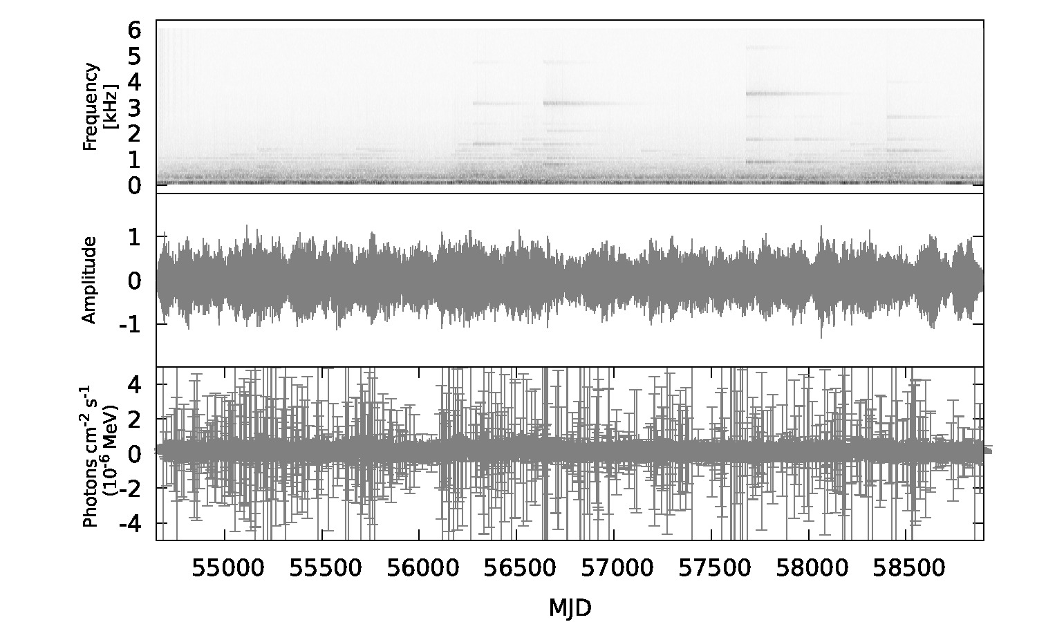
3.3.1 Waveforms and spectrograms
The visual representation of the objects were represented in three ways: the light curves, the waveforms and the spectrograms. All plots are paired in the dimension of time.
For the data of each blazar, these waveforms, are a representation of a sound wave in function of time, where the amplitude represents the volume of the sound. For all studied blazars, since the datasets were normalised, then the maximum amplitude is 1.
The spectrograms provide information about the frequencies that make up a sound, in which we can appreciate the graphic representation of how the frequency varies over time. Understanding the frequency, as the pitch of the instrument (in this case a tinkle bell instrument), the faster the wave repeats itself (given the frequency), the higher the pitch of the note.
It is important to mention that any physical object or phenomenon that emits noise periodically (hundreds or thousands of times per second) must have a perceptible tone. However, not all sound is periodic. For example, since white noise represents static sound, it is just a uniform distribution of audible frequencies, or Gaussian distribution. Therefore, because white noise is non-periodic, it does not have a noticeable pitch.
4 Discussion
Using a bell as a sonification instrument in this part of the production enhances clarity and auditory distinction. Its resonant tone makes it easier to perceive important events in the data without blending with other sounds.
Additionally, its sharp attack (well-defined onset) allows for precise marking of specific points in time, which is particularly useful for sonifying time series or discrete events. The bell also generates harmonics that enrich the tonal representation of data variations, helping to distinguish between different values or categories.
For example, in the light curves presented here, higher flux values translate into a more intense or higher-amplitude sound that gradually fades over time, fully covering the gaps in the curve. While these changes are evident in waveforms, they may go unnoticed in light curves. However, the ear can detect abrupt shifts in intensity or volume.
This is the advantage of sonification: what escapes the eye can be perceived by the ear.
Synchronising the three plots (light curve, waveform, and spectrogram) along the time axis provides a multidimensional representation of the data. The light curve illustrates how the intensity or flux of the signal changes over time, offering a global view of the source’s luminosity or intensity. This makes it possible to identify transient events such as peaks, dips, eclipses, explosions, or periodic variations.
The waveform, on the other hand, captures the full temporal evolution of the signal with high amplitude resolution. It acts as a detailed zoom into the temporal variations that might not be visible in the light curve. This allows for the analysis of precise dynamics, such as rapid pulses, subtle oscillations, or specific shapes. It also helps to distinguish noise from real signals and correlate light curve peaks with their exact amplitude and timing.
The spectrogram decomposes the signal into its frequency components, showing how they evolve over time. It helps to identify events linked to specific frequency bands, such as peaks or oscillation modes and distinguishes noise, characterised by specific spectral patterns, from significant signals.
Combining these three plots provides a multiscale analysis:
-
•
The light curve offers a general view of the signal’s behaviour over time.
-
•
The waveform adds fine detail about amplitude variations.
-
•
The spectrogram reveals frequency properties, uncovering patterns not evident in the other two.
This integrated approach enables the correlation of complex events. For instance, a peak in the light curve can be examined in the waveform to determine if it represents a sudden event and in the spectrogram to check for associated frequency changes. This is relevant for identifying specific physical phenomena, such as periodic pulses, spectral bursts, or emission changes, often observed in the study of blazars or binary stars.
Moreover, this combination is key to differentiate real signals from noise. An apparent change in the light curve that turns out to be noise can be confirmed using the waveform and spectrogram if no clear patterns in amplitude or frequency are detected. For transient events or explosions, the light curve can measure the event’s total duration and peak intensity, the waveform provides details about the pulse dynamics, and the spectrogram highlights the specific frequency bands involved.
For example, in the observation of a blazar, the light curve tracks global brightness variations, the waveform reveals rapid underlying pulses invisible on a larger scale, and the spectrogram identifies harmonic components or specific spectral features.
The synchronised combination of light curve, waveform, and spectrogram provides a comprehensive and integrated view of the data: intensity, temporal dynamics, and frequency structure. This enhanced analysis, facilitates the identification of complex events and improves the interpretation of physical phenomena.
As mentioned in the Introduction, there are already several works on data sonification in astronomy. These works provide important information from the perspective of sonifying the image, since the areas with the highest light intensity can be distinguished with the ear. In addition, they have a high pedagogical value, since they allow the public to have a didactic and playful approach to astronomy.
However, these works do not show on the time line how are the variations, trends, cyclicity, periodicity, seasonality of the phenomena or of the radiative processes. In this sense, the route that we have taken is that of sonification of the time series, or light curves, and the exercise that we have carried out has been on nine active galaxies that contain a supermassive black hole in their nucleus, an accretion disk that surrounds it, and a relativistic jet, so the radiation emission from these objects is multifrequency. Thus, sonification data for the Mrk 501, Mrk 1501, Mrk 421, BL Lacerta, AO 0235+164, 3C 66A (PKS 0219+428), OJ 049 (PKS 0829+046), OJ 287, and PKS J2134-0153 blazars were presented with their associated light curves, waveforms and spectrograms.
5 Conclusions
This study presents a multifrequency exploration of blazars, combining visualisation techniques (light curves, waveforms, and spectrograms) with sonification as complementary tools for representing and analysing their multifrequency variability. The integration of these methods not only enables a richer interpretation of the data but also provides perspectives for scientific communication, particularly for visually impaired communities.
Although this approach does not aim to definitively demonstrate periodicities, the auditory representation offers an innovative way to identify potential patterns, correlate events across different time scales, and explore the complex dynamics of these astrophysical objects. This work lays the groundwork for future research to delve deeper into the potential of sonification to highlight regularities and transient phenomena in astronomical data.
This multimodal approach contributes to a more inclusive and diverse understanding of blazar behaviour, paving the way to expand scientific analysis through methods that integrate both visual and auditory perception.
The radiation processes in the studied galaxies are multifrequency, so the data we have processed for sonification correspond to radio, optical, X-ray, and gamma-ray bands. Thus, the auditor can listen to the recorded signals that are emitted due to the radiative processes that distinguish the components of the active nucleus of the galaxy. Data were obtained from seven observatories: UMRAS, OVRO, AAVSO, Astrogeo-VLBI, Swift, Fermi, and ZTF.
The graphs presented for each of the blazars are specially useful for detecting changes over time, as well as getting a closer idea of sonification in visual terms. In these one can visualise what has been sounded, the changes in intensity (volume) and frequency (tone).
It is important to say that other fields in astronomy in which the sonification of data is present are in matters of education and public participation. There is a record of how sonifying images is impacting the dissemination of astronomy, and how citizen participation is increasing (Zanella et al., 2022).
The sonification of data is a way with which substantial information can be extracted, such as the search for periodicities, power increases, regularities, absences of information, etc. In addition to visualising the data, we have sonified it with the purpose of disseminating our advances to an even broader spectrum of society, at the same time that we investigate auditory events through the sense of hearing that help to distinguish periodicities.
Thus, the central interest of this work has been to disseminate the analysis of astrophysical data from a technique that is attractive to science in general, which is listening to the phenomena. In this sense, this is a work to bring the general public closer to astrophysics, from the sonification of the light curves of the active nuclei of galaxies, but also from the concern to socially include in science sectors of the population are blind or vision impaired (BVI) (Pérez-Montero, 2019).
Acknowledgements
This work was supported by a PAPIIT DGAPA-UNAM grants IN110522 and IN118325. GMG and SM acknowledge support from Secihti (378460,26344). We thank the OVRO 40-m monitoring program (Richards et al., 2011) for the radio database. The public OVRO database is supported by private funding from the California Institute of Technology and the Max Planck Institute for Radio Astronomy, and by NASA grants NNX08AW31G, NNX11A043G, and NNX14AQ89G and NSF grants AST-0808050 and AST- 1109911. We also thank the variable star database of observations from the AAVSO International Database contributed by observers worldwide. We thank the public data observations from the Swift data archive and the Fermi Gamma-Rays Space Telescope collaboration for the public database used in this work.
The operation of UMRAO is supported by funds from the University of Michigan Department of Astronomy, which we acknowledge too. ‘This research has made use of data from the University of Michigan Radio Astronomy Observatory which has been supported by the University of Michigan and by a series of grants from the National Science Foundation, most recently AST-0607523’.
We thank the use of archival calibrated VLBI data from the Astro-geo Center database maintained by Leonid Petrov.
This work has used observations obtained with the Samuel Oschin 48-inch Telescope at the Palomar Observatory as part of the Zwicky Transient Facility project. ZTF is supported by the National Science Foundation under Grant No. AST-1440341 and a collaboration including Caltech, IPAC, the Weizmann Institute for Science, the Oskar Klein Center at Stockholm University, the University of Maryland, the University of Washington, Deutsches Elektronen-Synchrotron and Humboldt University, Los Alamos National Laboratories, the TANGO Consortium of Taiwan, the University of Wisconsin at Mil- waukee, and Lawrence Berkeley National Laboratories. Operations are conducted by COO, IPAC, and UW. This work has made use of publicly available data from ZTF (https://irsa.ipac.caltech.edu/Missions/ztf.html).
Data Availability
The data underlying this article are available in the article and in its online supplementary material, together with the complementary webpage: https://www.guijongustavo.org/datasonification.
References
- Abbott et al. (2016) Abbott B. P., et al., 2016, Physical review letters, 116, 061102
- Abdo et al. (2009) Abdo A. A., et al., 2009, Science, 323, 1688
- Abdo et al. (2011a) Abdo A. A., et al., 2011a, ApJ, 727, 129
- Abdo et al. (2011b) Abdo A. A., et al., 2011b, ApJ, 736, 131
- Aller et al. (1985) Aller H. D., Aller M. F., Latimer G. E., Hodge P. E., 1985, ApJS, 59, 513
- Arsioli & Polenta (2018) Arsioli B., Polenta G., 2018, A&A, 616, A20
- Atwood et al. (2009) Atwood W., et al., 2009, The Astrophysical Journal, 697, 1071
- Berti (2016) Berti E., 2016, Physics Online Journal, 9, 17
- Bhatta (2019) Bhatta G., 2019, MNRAS, 487, 3990
- Blandford et al. (2019) Blandford R., Meier D., Readhead A., 2019, ARA&A, 57, 467
- Böttcher et al. (2005) Böttcher M., et al., 2005, ApJ, 631, 169
- Cabrera et al. (2013) Cabrera J. I., Coronado Y., Benítez E., Mendoza S., Hiriart D., Sorcia M., 2013, MNRAS, 434, L6
- Chandra (2003) Chandra 2003, Chandra "Hears" A Black Hole For The First Time, https://chandra.harvard.edu/press/03_releases/press_090903.html
- Chandra (2020) Chandra 2020, Data Sonification: Sounds from Around the Milky Way, https://chandra.harvard.edu/press/03_releases/press_090903.html
- Cohen et al. (1987) Cohen R. D., Smith H. E., Junkkarinen V. T., Burbidge E. M., 1987, ApJ, 318, 577
- D’Elia et al. (2015) D’Elia V., Padovani P., Giommi P., Turriziani S., 2015, MNRAS, 449, 3517
- Della Ceca et al. (1990) Della Ceca R., Palumbo G., Persic M., Boldt E., Marshall E., De Zotti G., 1990, The Astrophysical Journal Supplement Series, 72, 471
- Dorner et al. (2017) Dorner D., et al., 2017, PoS, ICRC2017, 609
- Errando et al. (2009) Errando M., Lindfors E., Mazin D., Prandini E., Tavecchio F., 2009, arXiv e-prints, p. arXiv:0907.0994
- Falomo (1991) Falomo R., 1991, AJ, 102, 1991
- Fichtel (1994) Fichtel C. E., 1994, ApJS, 90, 917
- Fiorucci, M. & Tosti, G. (1996) Fiorucci, M. Tosti, G. 1996, Astron. Astrophys. Suppl. Ser., 116, 403
- Fomalont et al. (2000) Fomalont E. B., Frey S., Paragi Z., Gurvits L. I., Scott W. K., Taylor A. R., Edwards P. G., Hirabayashi H., 2000, ApJS, 131, 95
- Fraija et al. (2017) Fraija N., et al., 2017, The Astrophysical Journal Supplement Series, 232, 7
- Friendly (2008) Friendly M., 2008, in , Handbook of data visualization. Springer, pp 15–56
- Graham et al. (2019) Graham M. J., et al., 2019, PASP, 131, 078001
- Grond & Berger (2011) Grond F., Berger J., 2011, in , The sonification handbook
- Guttman et al. (2005) Guttman S. E., Gilroy L. A., Blake R., 2005, Psychological science, 16, 228
- Hegg et al. (2018) Hegg J. C., Middleton J., Robertson B. L., Kennedy B. P., 2018, Heliyon, 4, e00532
- Hermann (2008) Hermann T., 2008.
- Hoffmeister (1929) Hoffmeister C., 1929, Astronomische Nachrichten, 236, 233
- Jansky (1933) Jansky K. G., 1933, Popular Astronomy, 41, 548
- Kellermann et al. (2020) Kellermann K. I., Bouton E. N., Brandt S. S., 2020, Open Skies: The National Radio Astronomy Observatory and Its Impact on US Radio Astronomy. Springer Nature
- Kramer et al. (1999) Kramer G., Walker B., Bargar R., for Auditory Display I. C., 1999, Sonification Report: Status of the Field and Research Agenda. International Community for Auditory Display, https://books.google.com.mx/books?id=Kv7yNwAACAAJ
- (35) LIGO Kernel Description, https://www.ligo.caltech.edu/video/ligo20160211v2#:~:text=As%20the%20black%20holes%20spiral,sound%20like%20a%20bird’s%20chirp
- Lainela et al. (1999) Lainela M., et al., 1999, ApJ, 521, 561
- Magallanes-Guijón & Mendoza (2022) Magallanes-Guijón G., Mendoza S., 2022, arXiv e-prints, p. arXiv:2210.15884
- Magallanes-Guijón (2020) Magallanes-Guijón G., 2020, Fermi-Tools Workshop: Light Curves, doi:10.13140/RG.2.2.25262.87365
- Mark (2016) Mark C. W., 2016, MIDITime Software, https://pypi.org/project/miditime
- Markarian et al. (1989) Markarian B. E., Lipovetsky V. A., Stepanian J. A., Erastova L. K., Shapovalova A. I., 1989, Soobshcheniya Spetsial’noj Astrofizicheskoj Observatorii, 62, 5
- Masetti (2013) Masetti M., 2013, Can You Hear a Black Hole?, https://asd.gsfc.nasa.gov/blueshift/index.php/2013/10/29/maggies-blog-can-you-hear-a-black-hole/
- Mattox (1998) Mattox J. R., 1998, in Zensus J. A., Taylor G. B., Wrobel J. M., eds, Astronomical Society of the Pacific Conference Series Vol. 144, IAU Colloq. 164: Radio Emission from Galactic and Extragalactic Compact Sources. p. 39
- Miller et al. (1978) Miller J. S., French H. B., Hawley S. A., 1978, ApJ, 219, L85
- Moretti et al. (2005) Moretti A., et al., 2005, in Siegmund O. H. W., ed., Society of Photo-Optical Instrumentation Engineers (SPIE) Conference Series Vol. 5898, UV, X-Ray, and Gamma-Ray Space Instrumentation for Astronomy XIV. pp 360–368, doi:10.1117/12.617164
- Morgan et al. (1997) Morgan E. H., Remillard R. A., Greiner J., 1997, ApJ, 482, 993
- Mukherjee et al. (1997) Mukherjee R., et al., 1997, ApJ, 490, 116
- NASA (2022) NASA 2022, Explore - From Space to Sound, https://www.nasa.gov/content/explore-from-space-to-sound
- Oke & Gunn (1974) Oke J. B., Gunn J. E., 1974, ApJ, 189, L5
- Padovani et al. (2012) Padovani P., Giommi P., Polenta G., Turriziani S., D’Elia V., Piranomonte S., 2012, arXiv e-prints, p. arXiv:1205.0647
- Parvizi et al. (2018) Parvizi J., Gururangan K., Razavi B., Chafe C., 2018, Epilepsia, 59, 877
- Penzias & Wilson (1965) Penzias A. A., Wilson R. W., 1965, ApJ, 142, 419
- Pérez-Montero (2019) Pérez-Montero E., 2019, Nature Astronomy, 3, 114
- Richards et al. (2011) Richards J. L., et al., 2011, ApJS, 194, 29
- Sargent & Searle (1970) Sargent W. L. W., Searle L., 1970, ApJ, 162, L155
- Sawe et al. (2020) Sawe N., Chafe C., Treviño J., 2020, Frontiers in Communication, 5, 46
- Shi et al. (2007) Shi W., Liu X., Song H., 2007, Ap&SS, 310, 59
- Smith et al. (2009) Smith P. S., Montiel E., Rightley S., Turner J., Schmidt G. D., Jannuzi B. T., 2009, Coordinated Fermi/Optical Monitoring of Blazars and the Great 2009 September Gamma-ray Flare of 3C 454.3, doi:10.48550/ARXIV.0912.3621, https://arxiv.org/abs/0912.3621
- Spinrad & Smith (1975) Spinrad H., Smith H. E., 1975, The Astrophysical Journal, 201, 275
- Torres-Zafra et al. (2018) Torres-Zafra J., Cellone S. A., Buzzoni A., Andruchow I., Portilla J. G., 2018, MNRAS, 474, 3162
- Truebenbach & Darling (2017) Truebenbach A. E., Darling J., 2017, The Astrophysical Journal Supplement Series, 233, 3
- Ulrich et al. (1975) Ulrich M. H., Kinman T. D., Lynds C. R., Rieke G. H., Ekers R. D., 1975, ApJ, 198, 261
- Ulrich et al. (1997) Ulrich M.-H., Maraschi L., Urry C. M., 1997, Annual Review of Astronomy and Astrophysics, 35, 445
- Valtonen et al. (2006) Valtonen M. J., et al., 2006, ApJ, 643, L9
- Vogt (2008) Vogt K., 2008, in inProc. of SysMus-1st International Conference of Students of Systematic Musicology, Graz, Austria.
- Zanella et al. (2022) Zanella A., Harrison C. M., Lenzi S., Cooke J., Damsma P., Fleming S. W., 2022, Nature Astronomy, 6, 1241
- von Montigny et al. (1995) von Montigny C., et al., 1995, ApJ, 440, 525