\headers

Exploring and Analyzing Wildland Fire Data via Machine Learning TechniquesD. Dulal, J. Charney, M. Gallagher, Carmeliza Navasca, N. Skowronski

Exploring and Analyzing Wildland Fire Data via Machine Learning Techniques

Dipak Dulal Department of Mathematics, University of Alabama at Birmingham, Birmingham, AL 35294 (, ) [email protected] [email protected] Joseph J. Charney USDA Forest Service, Northern Research Station - Climate, Fire, and Carbon Cycle Sciences, Lansing, MI 48910 () [email protected] Michael Gallagher USDA Forest Service, Northern Research Station - Climate, Fire, and Carbon Cycle Sciences, New Lisbon, NJ 08064 () [email protected] Carmeliza Navasca¹¹footnotemark: 1 Nicholas Skowronski USDA Forest Service, Northern Research Station - Climate, Fire, and Carbon Cycle Sciences, Morgantown, WV 26505 () [email protected]

Abstract

This research project investigated the correlation between a 10 Hz time series of thermocouple temperatures and turbulent kinetic energy (TKE) computed from wind speeds collected from a small experimental prescribed burn at the Silas Little Experimental Forest in New Jersey, USA. The primary objective of this project was to explore the potential for using thermocouple temperatures as predictors for estimating the TKE produced by a wildland fire. Machine learning models, including Deep Neural Networks, Random Forest Regressor, Gradient Boosting, and Gaussian Process Regressor, are employed to assess the potential for thermocouple temperature perturbations to predict TKE values. Data visualization and correlation analyses reveal patterns and relationships between thermocouple temperatures and TKE, providing insight into the underlying dynamics. The project achieves high accuracy in predicting TKE by employing various machine learning models despite a weak correlation between the predictors and the target variable. The results demonstrate significant success, particularly from regression models, in accurately estimating the TKE. The research findings contribute to fire behavior and smoke modeling science, emphasizing the importance of incorporating machine learning approaches and identifying complex relationships between fine-scale fire behavior and turbulence. Accurate TKE estimation using thermocouple temperatures allows for the refinement of models that can inform decision-making in fire management strategies, facilitate effective risk mitigation, and optimize fire management efforts. This project highlights the valuable role of machine learning techniques in analyzing wildland fire data, showcasing their potential to advance fire research and management practices.

keywords:

Wildland Fire, Machine Learning, Turbulence, and Fire Behavior

1 Introduction

Wildland fire is a natural and essential ecological process. Over the years, however, the frequency and area of wildfires have increased, which has led to dire consequences for public health and our ecological systems [17]. This phenomenon can be attributed to climate change, that is, fuel accumulation due to fire suppression. Over the past decade, wildfires have intensified, with 10 million acres burned annually in 2015, 2017, and 2020 [1]. Additionally, vegetation-related mortality is estimated to cause approximately 30,000 premature deaths annually [22]. To address this issue, a better understanding of the fundamental physical mechanisms of fire behavior is necessary, from the microscopic level (individual fuel particles) to entire landscapes. To this end, researchers have conducted highly instrumented field experiments [15] and developed computational fluid dynamics models [6] to improve our decision-making in the future. For example, Giannaros et al.[13] used coupled atmosphere-fire modeling to forecast fire spread, simulating a two-way interaction between fire and weather.
In this project, our primary objective was to investigate the intricate relationship between various fire characteristics and leverage the power of Artificial Intelligence and ML techniques to identify and estimate fire behavior, turbulence, and propagation. By examining the correlation between thermocouple temperature measurement and TKE, this research aims to provide valuable information on the dynamic nature of wildland fire behavior and its impact on local atmospheric conditions[6]. We implemented our models on the novel data generated from the wildland fire combustion process. See the data section 3.1. Figure 1 represents the architecture of our entire project.

Figure 1: Architecture of the Project

1.1 Related Works

Experts have recently studied wildland fires and their behavior using cutting-edge technologies such as deep neural networks, artificial intelligence, and machine learning. Classification and regression models have successfully predicted wildfires from remote sensing data, fire incident records, and explanatory variables such as vegetation, weather, and drought [18, 14]. DeCastro et al.[5] utilized synthetic aperture radar of band C, multispectral imagery, and tree mortality survey data to successfully estimate wildland fuel data by implementing the Random Forest model. The combination of satellite spatiotemporal data and transport models has been reliable in predicting $PM_{2.5}$ concentration in large fire events[20]. Mapulane Makhaba and Simon L Winberg[16]combined reinforcement[9] and supervised learning in the form of a Long-term Recurrent Convolutional Network (LRCN) to predict the spread of a large fire from its ignition point to the surrounding areas. An auto-encoder neural network (unsupervised machine learning) and coupled spatio-temporal auto-encoder (CSTAE) model have been implemented to train Sentinel 1 ground range detection (GRD) data to detect forest fires[8].

2 Contributions

Our study focuses on mainly three contributions

•

Temperature time series datasets collected from thermocouples in a 10x10m experimental fire grid at a frequency of 10 Hz have been primarily qualitatively analyzed in the past. However, our research has uncovered a correlation between these datasets and turbulence (TKE) values, highlighting the relationship between temperature fluctuations directly above the fire and nearby turbulence readings. We have developed a methodology to apply this analysis to similar experimental fires and other instruments. Studying the correlation between temperature and TKE has improved our understanding of how temperature changes due to wildfire combustion are linked to turbulence production. This knowledge helps evaluate existing tools and develop new ones for prescribed burns necessary for fuel reduction, forest management, and ecological maintenance.
•

This project utilized advanced machine learning and deep neural network models to analyze temperature fluctuations during the combustion process. The project successfully estimates the TKE of wildland fires by identifying patterns in these fluctuations. Introducing AI techniques to spatiotemporal wildland fire datasets and estimating fire turbulence and propagation behavior are new and innovative approaches.
•

We applied our correlation analysis and TKE estimation algorithms to the Burn20 dataset, which consisted of eight sets of data: B1, C1, B2, C2, B3, C3, B4, and C4, as well as their combinations B1C1, B2C2, B3C3, and B4C4, collected from different trusses mounted on different coordinates. Our findings indicated that the datasets did not follow the same pattern and that the positions and heights of the trusses played a significant role in correlation analysis with TKE and estimation algorithms.

3 Data

3.1 Data Aquisition

We obtained data from a set of highly instrumented intermediate-scale fire experiments conducted at the Silas Little Experimental Forest(SLEF) in New Lisbon, New Jersey. All experiments in the series were carried out within 10m $\times$ 10m research plots located within the SLEF research plantation, spanning from March 2018 to June 20l9 [15, 12, 4]. Figures 2(a),2(b),2(c), and 2(d) illustrate the equipment setup’s design, the anemometer’s placement, and images, both visible and infrared, taken during the burning period. During the experiments, data from multiple attributes of the fire were characterized in different formats: multi-band imagery with digital numbers, CSV files, and TIF data. However, our particular emphasis was on analyzing the sonic anemometer and thermocouple temperature data stored in CSV format. The main focus of the analysis presented here revolved around the B and C trusses, each subdivided into four distinct groups, as illustrated in Figure 2.

Refer to caption — (a) Complete instruments set up

3.2 Data Preprocessing and Visualization

We implemented two datasets, Burn20 B and C, each with four clusters from the trusses B1, B2, B3, B4, and C1, C2, C3, and C4, respectively. We divided the data into three parts: pre-burn, burn, and post-burn, based on the timestamps. Our correlation and machine learning model exploration concentrates on the burn period section. We computed TKE as our target variables from the perturbed windspeeds.

(1)

\displaystyle U^{\prime}=U-\bar{U},\hskip 2.84544ptV^{\prime}=V-\bar{V},\hskip 2.84544ptW^{\prime}=W-\bar{W}

where $\bar{U},\bar{U}$ , and $\bar{W}$ respectively are the average of the wind speeds U, V, and W representing east-west,north-south, and up-down direction during the pre-born period truncated between $-50^{0}$ and $+50^{0}$ Celcius. We computed TKE [7] as the following equation:

(2)

\displaystyle TKE=\frac{1}{2}(U^{{}^{\prime}2}+V^{{}^{\prime}2}+W^{{}^{\prime}2})

We observed the graphical representation of the computed TKE, which had a bit more fluctuation, and calculated the 10-point moving average of TKE. Figure 3 displays the wind speeds, the TKE, and the TKE moving average ( $TKE\_MA$ ).We focused on observing and executing our models on the anemometer temperatures( ${}^{o}C)$ $T_{1},T_{2},T_{3},T_{4},T_{5},T_{6}$ , and $T_{7}$ from the trusses mounted at 0, 5, 10, 20, 30, and 50 cm above the fuel beds. Figure 4 represents the cleaned thermocouple temperatures collected from different trusses. The spikes on the graph reflect the fire intensity during the burn.

4 Correlation Analysis

we calculated Pearson’s Correlation coefficient [21] and Spearman’s Rank Correlation coefficients [10]. These calculations were applied to discern the interrelation between thermocouple temperatures and TKE within each distinct cluster of the dataset. Furthermore, we extended this analysis to combinations derived from pairs of individual clustersThe main goal of this study is to thoroughly examine the complex connections between the turbulence features of wildland fires and their subsequent behavior and spread patterns, with a particular focus on correlations with thermocouple and sonic temperatures. Figures 5(a) and 5(b) show Pearson’s and Spearman’s rank correlation coefficients between thermocouple temperatures and TKE for datasets B and C. The correlation for datasets B4 and C4 is significantly stronger and positive, even though the overall coefficients remain subpar. On the other hand, datasets B1 and C1 have the most extreme negative correlation between the two variables. Figures 6(a) and 6(b) demonstrate that combining two sets from four trusses of B and C, B4C4, has the highest positive correlation coefficients.

5 Methodology

5.1 Problem Formulation

Let our dataset be represented as

(3)

\displaystyle\mathcal{D}=\{(\mathbf{x}^{(i)},y^{(i)})\}_{i=1}^{N}

where $\mathbf{x}^{(i)}\in\mathbb{R}^{8}$ such that

\mathbf{x}^{(i)}=[T1^{(i)},T2^{(i)},T3^{(i)},T4^{(i)},T5^{(i)},T6^{(i)},T7^{(i)},\text{sonic}\_T^{(i)}]

And $y^{(i)}\in\mathbb{R}$ is the corresponding output,i.e. TKE.

Our objective is to train a machine learning model $f(\mathbf{x};\bm{\theta})$ parametrized by $\bm{\theta}$ to approximate the function $g:\mathbb{R}^{8}\to\mathbb{R}$ that maps input vectors to TKE values. The objection function for our optimization problem is formulated as follows:

(4)

\displaystyle\bm{\theta}^{*}=\arg\min_{\bm{\theta}}\left(\sum_{i=1}^{N}L(y^{(i)},f(\mathbf{x}^{(i)};\bm{\theta}))+\lambda R(\bm{\theta})\right)

where $L$ is a loss function $R$ is a regularization term. We used on our algorithm ridge regression(L2) and Lasso Regression(L1) regularizers as necessary to our machine learning models, and $\lambda>0$ is the regularization strength.

5.2 Model Implementation and Description

5.2.1 Deep Neural Network (DNN)

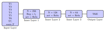
The deep neural network (DNN) comprises an input layer, three hidden layers, and an output layer. The layers are interconnected through weights and biases, optimized to minimize the objective function[11]. Figure 7 reflects our DNN algorithm structure.

5.2.2 Random Forest Regressor(RF)

Random Forest aggregates the predictions of multiple decision trees, offering an ensemble prediction:

(5)

\displaystyle\hat{y}=\frac{1}{M}\sum_{m=1}^{M}T_{m}(\bm{T})

where $M$ is the number of trees.

5.2.3 K-Nearest Neighbors (KNN) Regressor

KNN predicts TKE by averaging the values of the k-nearest training samples. Given a dataset $\mathcal{D}$ and $y^{(i)}\in\mathbb{R}$ is the corresponding TKE output, the k-NN regressor estimates the TKE as:

(6)

\displaystyle\hat{y}=\frac{1}{k}\sum_{i\in\mathcal{N}_{k}(\bm{T_{*}})}y^{(i)}

where $\mathcal{N}_{k}(\bm{T_{*}})$ denotes the set of k-nearest neighbors.

5.2.4 Gradient Boosting (GB) Regressor

GB constructs trees sequentially:

(7)

\displaystyle\hat{y}(\bm{T})=\sum_{j=1}^{J}\rho_{j}T_{j}(\bm{T})

with $\rho_{j}$ as step sizes and $J$ as the boosting stages.

5.2.5 XGBoost Regressor(XGB)

XGBoost’s objective integrates the number of leaves and leaf scores, further regularized by the L1 and L2 norms [3]:

(8)

\displaystyle\mathcal{O}(\Theta)=\sum_{i=1}^{n}L(y^{(i)}i,f(\bm{x^{(i)}};\Theta))+\gamma T+\frac{1}{2}\alpha\lVert w\rVert^{2}

where $T$ is the number of leaves and $w$ represents leaf scores.

5.2.6 Gaussian Process Regression with Regularization

A Gaussian Process (GP) [19] defines a distribution over functions, which can be fully specified by its mean function $m(\mathbf{x})$ and covariance function $k(\mathbf{x},\mathbf{x}^{\prime})$ . In our approach, we assume a zero mean function without loss of generality, and a suitable kernel is selected for the covariance function. The predictive distribution of a GP at a new point $\mathbf{x}_{*}$ is given by,

(9)

\displaystyle p(y_{*}|\mathbf{x}_{*},\mathcal{D})=\mathcal{N}(y_{*}|\mu_{*},\sigma^{2}_{*}),

where

(10)		$\displaystyle\mu_{*}$	$\displaystyle=\mathbf{k}_{*}^{T}(\mathbf{K}+\sigma_{n}^{2}\mathbf{I})^{-1}\mathbf{y},$
(11)		$\displaystyle\sigma^{2}_{*}$	$\displaystyle=k(\mathbf{x}_{},\mathbf{x}_{})-\mathbf{k}_{}^{T}(\mathbf{K}+\sigma_{n}^{2}\mathbf{I})^{-1}\mathbf{k}_{},$

with $\mathbf{k}_{*}$ being the covariance between the training inputs and $\mathbf{x}_{*}$ , $\mathbf{K}$ the covariance matrix of the training inputs, and $\sigma_{n}^{2}$ the noise term.

Lasso ( $L_{1}$ ) and Ridge ( $L_{2}$ ) regularization techniques are incorporated into the GP model to mitigate overfitting and enhance model generalization. The modified objective function with the regularizers is represented as:

(12)

\displaystyle\mathcal{L}(\mathbf{w})=\frac{1}{2}(\mathbf{y}-\mathbf{Kw})^{T}(\mathbf{y}-\mathbf{Kw})+\alpha\|\mathbf{w}\|_{1}+\beta\|\mathbf{w}\|_{2}^{2},

where $\mathbf{w}$ are the weights, $\alpha$ and $\beta$ are the regularization coefficients for Lasso and Ridge regularization, respectively.

6 Results and Evaluation

We initially attempted to estimate TKE using a Deep Neural Network (DNN). We conducted experiments with various numbers of layers and adjusted hyperparameters to obtain the best results. Ultimately, we found that three inner layers and lasso regression regularization in the third layer produced the best results despite having lower accuracy and efficiency than other ensemble models. Detailed evaluations of $R^{2}$ values of all models over individual datasets and the combination of two from each set are presented in Tables 1 and 2, respectively. Our findings show that DNN models are weaker compared to other models over all datasets, with GPR being the best for each dataset.

	Burn20 B				Burn20 C
ML Models	B1	B2	B3	B4	C1	C2	C3	C4
	Test (%)
DNN	52.6	52.4	60.2	64.6	60.9	61.5	63.2	61.2
RFR	84.8	86.0	81.2	84.5	87.3	85.6	86.6	84.3
KNN	93.6	93.8	92.4	91.4	82.5	81.3	92.2	88.4
GBR	79.4	80.9	75.3	79.5	81.1	81.3	82.1	81.5
GPR	93.7	92.6	92.4	90.4	82.4	81.3	87.2	84.4
XGB	92.4	90.6	89.7	89.3	92.2	89.4	92.4	87.1
	Val (%)
DNN	52.6	52.4	60.2	64.6	87.7	86.7	64.8	62.2
RFR	84.8	86.0	81.2	84.5	93.1	93.4	84.9	80.0
KNN	93.6	93.8	92.4	91.4	96.5	95.0	84.4	82.9
GBR	79.4	80.9	75.3	79.5	89.0	88.4	79.8	74.4
GPR	93.7	92.6	92.4	90.4	93.3	94.7	76.6	79.8
XGB	92.4	90.6	89.7	89.3	95.0	94.5	89.2	87.5

Table 1: ML prediction models comparison over

R^{2}

ML Models	B1C1(%)		B2C2(%)		B3C3(%)		B4C4(%)
ML Models	Test	Val	Test	Val	Test	Val	Test	Val
DNN	45.7	44.3	60.1	63.2	70.4	74.7	70.5	73.9
RFR	81.5	78.6	84.0	81.3	82.9	80.4	82.4	80.5
KNN	92.4	91.7	89.6	89.2	90.8	90.2	90.5	90.0
GBR	72.7	74.2	73.8	73.4	74.7	73.2	750.	73.6
GPR	92.0	89.8	91.1	89.4	90.3	91.01	90.1	91.0
XGB	91.5	90.9	89.8	89.6	90.1	89.8	89.2	87.1

Table 2: ML prediction models comparison over

R^{2}

on BC

To evaluate the performance of our models, we analyzed the residual plots and employed Kernel Density Estimation(KDE). KDE is a useful tool for visualizing data distribution over a continuous interval or period [2]. Our analysis revealed that the GPR model consistently exhibited a sharp peak at the 0 residual for all conditions, indicating superior performance. In contrast, the Random Forest model showed a broader distribution for almost all conditions. See figure 8.

The graph in figure 9 displays a steady decrease in errors, apart from some minor fluctuations on dataset B1C1.

The chart shown in figure 10 compares the predicted values of various machine learning models with actual data across four selected datasets. Each subplot displays the actual values in blue and the predicted values in orange. While all models show a decent level of adherence between actual and expected values across datasets, the GPR model has the most consistent results in this expanded dataset, especially in the B3 and B4C4 datasets.

The figure11 presents a performance comparison of six machine learning models across various data conditions using MSE and MAE metrics. Notably, GPR, KNN, and XGB consistently showcase superior predictive accuracy across most conditions. In contrast, DNN and RFR occasionally manifest higher errors, suggesting variability in model adaptability to different datasets.

7 Future Works and Conclusion

We investigated to explore the connections between thermocouple temperatures, sonic temperatures, and TKE. Although the correlation and covariance between the predictor variables and the target variable were not strong, our machine learning and deep learning algorithms could identify the hidden and intricate features of the predictor variables related to the target variable. Consequently, we were able to predict fire behavior accurately and spread through TKE estimation with the help of these algorithms. After a thorough hyperparameter tuning, exploration, and implementation of complex regularizers, we found that Gaussian Process Regressors were the most suitable model for estimating TKE with high precision and low error.
This study has revealed a connection between temperature and TKE time series that provides insight into how temperature changes caused by combustion are linked to the production of turbulence above and near a wildland fire. We determined that the correlation between the temperatures and TKE is not uniform across trusses, with some trusses contributing more than others. This knowledge will benefit wildland fire research scientists as they assess current tools and create new ones that fire managers can use to plan and carry out prescribed burns necessary for fuel reduction, forest management, and ecological restoration and upkeep.
In our subsequent research, we aim to delve deeper into the behavior and propagation of fires by synergizing high-dimensional IR image datasets with the complex physical behaviors of associated tools. Our primary emphasis will be on employing a rigorous Deep Neural Network methodology to analyze the Hyperspectral image datasets related to wildland fires.

8 Acknowledgments

This fellowship was funded by the National Science Foundation Oak Ridge Institute of Science and Education(NSF-ORISE) under the Mathematical Science Graduate Internship (MSGI). Data acquisition was funded by the US Department of Defense Strategic Environmental Research and Development Program Project RC-2641.

References

[1] in Wildfire Risk Report 2022, CoreLogic, ed., 2022, https://www.corelogic.com/intelligence/the-2022-wildfire-report/.
[2] T. K. Anderson, Kernel density estimation and k-means clustering to profile road accident hotspots, Accident Analysis & Prevention, 41 (2009), pp. 359–364, https://doi.org/https://doi.org/10.1016/j.aap.2008.12.014, https://www.sciencedirect.com/science/article/pii/S0001457508002340.
[3] T. Chen and C. Guestrin, Xgboost: A scalable tree boosting system, in Proceedings of the 22nd ACM SIGKDD International Conference on Knowledge Discovery and Data Mining, KDD ’16, New York, NY, USA, 2016, Association for Computing Machinery, p. 785–794, https://doi.org/10.1145/2939672.2939785, https://doi.org/10.1145/2939672.2939785.
[4] K. L. Clark et al., Multi-scale analyses of wildland fire combustion processes: Small-scale field experiments – three-dimensional wind and temperature, USDA, Research Data Archive, (2022), https://www.fs.usda.gov/rds/archive/catalog/RDS-2022-0081.
[5] A. L. DeCastro, T. W. Juliano, B. Kosović, H. Ebrahimian, and J. K. Balch, A computationally efficient method for updating fuel inputs for wildfire behavior models using sentinel imagery and random forest classification, Remote Sensing, 14 (2022), p. 1447, https://doi.org/10.3390/rs14061447, http://dx.doi.org/10.3390/rs14061447.
[6] A. Desai, S. Goodrick, and T. Banerjee, Investigating the turbulent dynamics of small-scale surface fires, Scientific Reports, 12 (2022), https://doi.org/10.1038/s41598-022-13226-w, https://doi.org/10.1038/s41598-022-13226-w.
[7] A. Desai, W. E. Heilman, N. S. Skowronski, K. L. Clark, M. R. Gallagher, C. B. Clements, and T. Banerjee, Features of turbulence during wildland fires in forested and grassland environments, Agricultural and Forest Meteorology, 338 (2023), p. 109501, https://doi.org/https://doi.org/10.1016/j.agrformet.2023.109501, https://www.sciencedirect.com/science/article/pii/S0168192323001922.
[8] T. Di Martino, B. Le Saux, R. Guinvarc’h, L. Thirion-Lefevre, and E. Colin, Detection of forest fires through deep unsupervised learning modeling of sentinel-1 time series, ISPRS International Journal of Geo-Information, 12 (2023), p. 332, https://doi.org/10.3390/ijgi12080332, http://dx.doi.org/10.3390/ijgi12080332.
[9] S. Ganapathi Subramanian and M. Crowley, Using spatial reinforcement learning to build forest wildfire dynamics models from satellite images, Frontiers in ICT, 5 (2018), https://doi.org/10.3389/fict.2018.00006, https://www.frontiersin.org/articles/10.3389/fict.2018.00006.
[10] T. D. Gauthier, Detecting trends using spearman’s rank correlation coefficient, Environmental Forensics, 2 (2001), pp. 359–362, https://doi.org/https://doi.org/10.1006/enfo.2001.0061, https://www.sciencedirect.com/science/article/pii/S1527592201900618.
[11] R. Ghali and M. A. Akhloufi, Deep learning approaches for wildland fires using satellite remote sensing data: Detection, mapping, and prediction, Fire, 6 (2023), https://doi.org/10.3390/fire6050192, https://www.mdpi.com/2571-6255/6/5/192.
[12] M. R. Ghallagher et al., Multi-scale analyses of wildland fire combustion processes: Small-scale field experiments – plot layout, and documentation, USDA, Research Data Archive, (2022), https://www.fs.usda.gov/rds/archive/catalog/RDS-2022-0083.
[13] T. M. Giannaros, V. Kotroni, and K. Lagouvardos, Iris – rapid response fire spread forecasting system: Development, calibration and evaluation, Agricultural and Forest Meteorology, 279 (2019), p. 107745, https://doi.org/https://doi.org/10.1016/j.agrformet.2019.107745, https://www.sciencedirect.com/science/article/pii/S0168192319303612.
[14] F. Huot, R. L. Hu, N. Goyal, T. Sankar, M. Ihme, and Y.-F. Chen, Next day wildfire spread: A machine learning dataset to predict wildfire spreading from remote-sensing data, IEEE Transactions on Geoscience and Remote Sensing, 60 (2022), pp. 1–13, https://doi.org/10.1109/TGRS.2022.3192974.
[15] C. L. et al., Multi-scale analyses of wildland fire combustion processes: Small-scale field experiments – temperature profile, USDA, Research Data Archive, (2022), https://www.fs.usda.gov/rds/archive/catalog/RDS-2022-0083.
[16] M. Makhaba and S. L. Winberg, Wildfire path prediction spread using machine learning, 2022 International Conference on Electrical, Computer and Energy Technologies (ICECET), (2022), pp. 1–5, https://api.semanticscholar.org/CorpusID:252166027.
[17] D. G. Neary, K. C. Ryan, and L. F. DeBano, Wildland fire in ecosystems: effects of fire on soils and water, tech. report, 2005, https://doi.org/10.2737/rmrs-gtr-42-v4, https://doi.org/10.2737%2Frmrs-gtr-42-v4.
[18] K. Pham, D. Ward, S. Rubio, D. Shin, L. Zlotikman, S. Ramirez, T. Poplawski, and X. Jiang, California wildfire prediction using machine learning, in 2022 21st IEEE International Conference on Machine Learning and Applications (ICMLA), 2022, pp. 525–530, https://doi.org/10.1109/ICMLA55696.2022.00086.
[19] C. E. Rasmussen and C. K. I. Williams, Gaussian Processes for Machine Learning, The MIT Press, 11 2005, https://doi.org/10.7551/mitpress/3206.001.0001, https://doi.org/10.7551/mitpress/3206.001.0001.
[20] C. E. Reid et al., Spatiotemporal prediction of fine particulate matter during the 2008 northern california wildfires using machine learning, Environmental Science & Technology, 49 (2015), pp. 3887–3896, https://doi.org/10.1021/es505846r. PMID: 25648639.
[21] P. Schober, C. Boer, and L. A. Schwarte, Correlation coefficients: Appropriate use and interpretation, Anesthesia & Analgesia, 126 (2018), https://journals.lww.com/anesthesia-analgesia/fulltext/2018/05000/correlation_coefficients__appropriate_use_and.50.aspx.
[22] G. R. van der Werf, J. T. Randerson, L. Giglio, T. T. van Leeuwen, Y. Chen, B. M. Rogers, M. Mu, M. J. E. van Marle, D. C. Morton, G. J. Collatz, R. J. Yokelson, and P. S. Kasibhatla, Global fire emissions estimates during 1997–2016, Earth System Science Data, 9 (2017), pp. 697–720, https://doi.org/10.5194/essd-9-697-2017, https://essd.copernicus.org/articles/9/697/2017/.