Exploration by Maximizing Rényi Entropy for Reward-Free RL Framework
Abstract
Exploration is essential for reinforcement learning (RL). To face the challenges of exploration, we consider a reward-free RL framework that completely separates exploration from exploitation and brings new challenges for exploration algorithms. In the exploration phase, the agent learns an exploratory policy by interacting with a reward-free environment and collects a dataset of transitions by executing the policy. In the planning phase, the agent computes a good policy for any reward function based on the dataset without further interacting with the environment. This framework is suitable for the meta RL setting where there are many reward functions of interest. In the exploration phase, we propose to maximize the Rényi entropy over the state-action space and justify this objective theoretically. The success of using Rényi entropy as the objective results from its encouragement to explore the hard-to-reach state-actions. We further deduce a policy gradient formulation for this objective and design a practical exploration algorithm that can deal with complex environments. In the planning phase, we solve for good policies given arbitrary reward functions using a batch RL algorithm. Empirically, we show that our exploration algorithm is effective and sample efficient, and results in superior policies for arbitrary reward functions in the planning phase.
1 Introduction
The trade-off between exploration and exploitation is at the core of reinforcement learning (RL). Designing efficient exploration algorithm, while being a highly nontrivial task, is essential to the success in many RL tasks (Burda et al. 2019b; Ecoffet et al. 2019). Hence, it is natural to ask the following high-level question: What can we achieve by pure exploration? To address this question, several settings related to meta reinforcement learning (meta RL) have been proposed (see e.g., Wang et al. 2016; Duan et al. 2016; Finn, Abbeel, and Levine 2017). One common setting in meta RL is to learn a model in a reward-free environment in the meta-training phase, and use the learned model as the initialization to fast adapt for new tasks in the meta-testing phase (Eysenbach et al. 2019; Gupta et al. 2018; Nagabandi et al. 2019). Since the agent still needs to explore the environment under the new tasks in the meta-testing phase (sometimes it may need more new samples in some new task, and sometimes less), it is less clear how to evaluate the effectiveness of the exploration in the meta-training phase. Another setting is to learn a policy in a reward-free environment and test the policy under the task with a specific reward function (such as the score in Montezuma’s Revenge) without further training with the task (Burda et al. 2019b; Ecoffet et al. 2019; Burda et al. 2019a). However, there is no guarantee that the algorithm has fully explored the transition dynamics of the environment unless we test the learned model for arbitrary reward functions. Recently, Jin et al. (2020) proposed reward-free RL framework that fully decouples exploration and exploitation. Further, they designed a provably efficient algorithm that conducts a finite number of steps of reward-free exploration and returns near-optimal policies for arbitrary reward functions. However, their algorithm is designed for the tabular case and can hardly be extended to continuous or high-dimensional state spaces since they construct a policy for each state.
The reward-free RL framework is as follows: First, a set of policies are trained to explore the dynamics of the reward-free environment in the exploration phase (i.e., the meta-training phase). Then, a dataset of trajectories is collected by executing the learned exploratory policies. In the planning phase (i.e., the meta-testing phase), an arbitrary reward function is specified and a batch RL algorithm (Lange, Gabel, and Riedmiller 2012; Fujimoto, Meger, and Precup 2019) is applied to solve for a good policy solely based on the dataset, without further interaction with the environment. This framework is suitable to the scenarios when there are many reward functions of interest or the reward is designed offline to elicit desired behavior. The key to success in this framework is to obtain a dataset with good coverage over all possible situations in the environment with as few samples as possible, which in turn requires the exploratory policy to fully explore the environment.
Several methods that encourage various forms of exploration have been developed in the reinforcement learning literature. The maximum entropy framework (Haarnoja et al. 2017) maximizes the cumulative reward in the meanwhile maximizing the entropy over the action space conditioned on each state. This framework results in several efficient and robust algorithms, such as soft Q-learning (Schulman, Chen, and Abbeel 2017; Nachum et al. 2017), SAC (Haarnoja et al. 2018) and MPO (Abdolmaleki et al. 2018). On the other hand, maximizing the state space coverage may results in better exploration. Various kinds of objectives/regularizations are used for better exploration of the state space, including information-theoretic metrics (Houthooft et al. 2016; Mohamed and Rezende 2015; Eysenbach et al. 2019) (especially the entropy of the state space, e.g., Hazan et al. (2019); Islam et al. (2019)), the prediction error of a dynamical model (Burda et al. 2019a; Pathak et al. 2017; de Abril and Kanai 2018), the state visitation count (Burda et al. 2019b; Bellemare et al. 2016; Ostrovski et al. 2017) or others heuristic signals such as novelty (Lehman and Stanley 2011; Conti et al. 2018), surprise (Achiam and Sastry 2016) or curiosity (Schmidhuber 1991).
In practice, it is desirable to obtain a single exploratory policy instead of a set of policies whose cardinality may be as large as that of the state space (e.g., Jin et al. 2020; Misra et al. 2019). Our exploration algorithm outputs a single exploratory policy for the reward-free RL framework by maximizing the Rényi entropy over the state-action space in the exploration phase. In particular, we demonstrate the advantage of using state-action space, instead of the state space via a very simple example (see Section 3 and Figure 1). Moreover, Rényi entropy generalizes a family of entropies, including the commonly used Shannon entropy. We justify the use of Rényi entropy as the objective function theoretically by providing an upper bound on the number of samples in the dataset to ensure that a near-optimal policy is obtained for any reward function in the planning phase.
Further, we derive a gradient ascent update rule for maximizing the Rényi entropy over the state-action space. The derived update rule is similar to the vanilla policy gradient update with the reward replaced by a function of the discounted stationary state-action distribution of the current policy. We use variational autoencoder (VAE) (Kingma and Welling 2014) as the density model to estimate the distribution. The corresponding reward changes over iterations which makes it hard to accurately estimate a value function under the current reward. To address this issue, we propose to estimate a state value function using the off-policy data with the reward relabeled by the current density model. This enables us to efficiently update the policy in a stable way using PPO (Schulman et al. 2017). Afterwards, we collect a dataset by executing the learned policy. In the planning phase, when a reward function is specified, we augment the dataset with the rewards and use a batch RL algorithm, batch constrained deep Q-learning (BCQ) (Fujimoto, Meger, and Precup 2019; Fujimoto et al. 2019), to plan for a good policy under the reward function. We conduct experiments on several environments with discrete, continuous or high-dimensional state spaces. The experiment results indicate that our algorithm is effective, sample efficient and robust in the exploration phase, and achieves good performance under the reward-free RL framework.
Our contributions are summarized as follows:
-
•
(Section 3) We consider the reward-free RL framework that separates exploration from exploitation and therefore places a higher requirement for an exploration algorithm. To efficiently explore under this framework, we propose a novel objective that maximizes the Rényi entropy over the state-action space in the exploration phase and justify this objective theoretically.
-
•
(Section 4) We propose a practical algorithm based on a derived policy gradient formulation to maximize the Rényi entropy over the state-action space for the reward-free RL framework.
-
•
(Section 5) We conduct a wide range of experiments and the results indicate that our algorithm is efficient and robust in the exploration phase and results in superior performance in the downstream planning phase for arbitrary reward functions.
2 Preliminary
A reward-free environment can be formulated as a controlled Markov process (CMP) 111 Although some literature use CMP to refer to MDP, we use CMP to denote a Markov process (Silver 2015) equipped with a control structure in this paper. which specifies the state space with , the action space with , the transition dynamics , the initial state distribution and the discount factor . A (stationary) policy parameterized by specifies the probability of choosing the actions on each state. The stationary discounted state visitation distribution (or simply the state distribution) under the policy is defined as . The stationary discounted state-action visitation distribution (or simply the state-action distribution) under the policy is defined as . Unless otherwise stated, we use to denote the state-action distribution. We also use to denote the distribution started from the state-action pair instead of the initial state distribution .
When a reward function is specified, CMP becomes the Markov decision process (MDP) (Sutton and Barto 2018) . The objective for MDP is to find a policy that maximizes the expected cumulative reward , where is the state value function. We indicate the dependence on to emphasize that there may be more than one reward function of interest. The policy gradient for this objective is (Williams 1992), where is the Q function.
Rényi entropy for a distribution is defined as , where is the probability mass or the probability density function on (and the summation becomes integration in the latter case). When , Rényi entropy becomes Hartley entropy and equals the logarithm of the size of the support of . When , Rényi entropy becomes Shannon entropy (Bromiley, Thacker, and Bouhova-Thacker 2004; Sanei, Borzadaran, and Amini 2016).
Given a distribution , the corresponding density model parameterized by gives the probability density estimation of based on the samples drawn from . Variational auto-encoder (VAE) (Kingma and Welling 2014) is a popular density model which maximizes the variational lower bound (ELBO) of the log-likelihood. Specifically, VAE maximizes the lower bound of , i.e., , where and are the decoder and the encoder respectively and is a prior distribution for the latent variable .
3 The objective for the exploration phase
The objective for the exploration phase under the reward-free RL framework is to induce an informative and compact dataset: The informative condition is that the dataset should have good coverage such that the planning phase generates good policies for arbitrary reward functions. The compact condition is that the size of the dataset should be as small as possible to ensure a successful planning. In this section, we show that the Rényi entropy over the state-action space (i.e., ) is a good objective function for the exploration phase. We first demonstrate the advantage of maximizing the state-action space entropy over maximizing the state space entropy with a toy example. Then, we provide a motivation to use Rényi entropy by analyzing a deterministic setting. At last, we provide an upper bound on the number of samples needed in the dataset for a successful planning if we have access to a policy that maximizes the Rényi entropy over the state-action space. For ease of analysis, we assume the state-action space is discrete in this section and derive a practical algorithm that deals with continuous state-action space in the next section.

Why maximize the entropy over the state-action space? We demonstrate the advantage of maximizing the entropy over the state-action space with a toy example shown in Figure 1. The example contains an MDP with two actions and five states. The first action always drives the agent back to the first state while the second action moves the agent to the next state. For simplicity of presentation, we consider a case with a discount factor , but other values are similar. The policy that maximizes the entropy of the state distribution is a deterministic policy that takes the actions shown in red. The dataset obtained by executing this policy is poor since the planning algorithm fails when, in the planning phase, a sparse reward is assigned to one of the state-action pairs that it visits with zero probability (e.g., a reward function that equals to on and equals to otherwise). In contrast, a policy that maximizes the entropy of the state-action distribution avoids the problem. For example, executing the policy that maximizes the Rényi entropy with over the state-action space, the expected size of the induced dataset is only 44 such that the dataset contains all the state-action pairs (cf. Appendix The toy example in Figure 1). Note that, when the transition dynamics is known to be deterministic, a dataset containing all the state-action pairs is sufficient for the planning algorithm to obtain an optimal policy since the full transition dynamics is known.
Why using Rényi entropy? We analyze a deterministic setting where the transition dynamics is known to be deterministic. In this setting, the objective for the framework can be expressed as a specific objective function for the exploration phase. This objective function is hard to optimize but motivates us to use Rényi entropy as the surrogate.
We define as the cardinality of the state-action space. Given an exploratory policy , we assume the dataset is collected in a way such that the transitions in the dataset can be treated as i.i.d. samples from , where is the state-action distribution induced by the policy .
In the deterministic setting, we can recover the exact transition dynamics of the environment using a dataset of transitions that contains all the state-action pairs. Such a dataset leads to a successful planning for arbitrary reward functions, and therefore satisfies the informative condition. In order to obtain such a dataset that is also compact, we stop collecting samples if the dataset contains all the pairs. Given the distribution from which we collect samples, the average size of the dataset is , where
| (1) |
which is a result of the coupon collector’s problem (Flajolet, Gardy, and Thimonier 1992). Accordingly, the objective for the exploration phase can be expressed as , where is the set of all the feasible policies. (Notice that due to the limitation of the transition dynamics, the feasible state-action distributions form only a subset of .) We show the contour of this function on in Figure 2a. We can see that, when any component of the distribution approaches zeros, increases rapidly forming a barrier indicated by the black arrow. This barrier prevents the agent to visit a state-action with a vanishing probability, and thus encourages the agent to explore the hard-to-reach state-actions.
However, this function involves an improper integral which is hard to handle, and therefore cannot be directly used as an objective function in the exploration phase. One common choice for a tractable objective function is Shannon entropy, i.e., (Hazan et al. 2019; Islam et al. 2019), whose contour is shown in Figure 2b. We can see that, Shannon entropy may still be large when some component of approaches zero (e.g., the black arrow indicates a case where the entropy is relatively large but ). Therefore, maximizing Shannon entropy may result in a policy that visits some state-action pair with a vanishing probability. We find that the contour of Rényi entropy (shown in Figure 2c/d) aligns better with and alleviates this problem. In general, the policy that maximizes Rényi entropy may correspond to a smaller than that resulted from maximizing Shannon entropy for different CMPs (more evidence of which can be found in Appendix An example to illustrate the advantage of using Rényi entropy).

Theoretical justification for the objective function. Next, we formally justify the use of Rényi entropy over the state-action space with the following theorem. For ease of analysis, we consider a standard episodic setting: The MDP has a finite planning horizon and stochastic dynamics with the objective to maximize the cumulative reward , where . We assume the reward function is deterministic. A (non-stationary, stochastic) policy specifies the probability of choosing the actions on each state and on each step. The state-action distribution induced by on the -th step is .
Theorem 3.1.
Denote as a set of policies , where and . Construct a dataset with trajectories, each of which is collected by first uniformly randomly choosing a policy from and then executing the policy . Assume
where and is an absolute constant. Then, there exists a planning algorithm such that, for any reward function , with probability at least , the output policy of the planning algorithm based on is -optimal, i.e., , where .
We provide the proof in Appendix Proof of Theorem 3.1. The theorem justifies that Rényi entropy with small is a proper objective function for the exploration phase since the number of samples needed to ensure a successful planning is bounded when is small. When , the bound becomes infinity. The algorithm proposed by Jin et al. (2020) requires to sample trajectories where hides a logarithmic factor, which matches our bound when . However, they construct a policy for each state on each step, whereas we only need policies which easily adapts for the non-tabular case.
4 Method
In this section, we develop an algorithm for the non-tabular case. In the exploration phase, we update the policy to maximize . We first deduce a gradient ascent update rule which is similar to vanilla policy gradient with the reward replaced by a function of the state-action distribution of the current policy. Afterwards, we estimate the state-action distribution using VAE. We also estimate a value function and update the policy using PPO, which is more sample efficient and robust than vanilla policy gradient. Then, we obtain a dataset by collecting samples from the learned policy. In the planning phase, we use a popular batch RL algorithm, BCQ, to plan for a good policy when the reward function is specified. One may also use other batch RL algorithms. We show the pseudocode of the process in Algorithm 1, the details of which are described in the following paragraphs.


Policy gradient formulation. Let us first consider the gradient of the objective function , where the policy is approximated by a policy network with the parameters denoted as . We omit the dependency of on . The gradient of the objective function is
| (2) | ||||
As a special case, when , the Rényi entropy becomes the Shannon entropy and the gradient turns into
| (3) | ||||
Due to space limit, the derivation can be found in Appendix Policy gradient of state-action space entropy. There are two terms in the gradients. The first term equals to with the reward or , which resembles the policy gradient (of cumulative reward) for a standard MDP. This term encourages the policy to choose the actions that lead to the rarely visited state-action pairs. In a similar way, the second term resembles the policy gradient of instant reward and encourages the agent to choose the actions that are rarely selected on the current step. The second term in (3) equals to . For stability, we also replace the second term in (2) with 222 We found that using this term leads to more stable performance empirically since this term does not suffer from the high variance induced by the estimation of (see also Appendix Practical implementation). . Accordingly, we update the policy based on the following formula where is a hyperparameter:
| (4) | ||||
Discussion. Islam et al. (2019) motivate the agent to explore by maximizing the Shannon entropy over the state space resulting in an intrinsic reward which is similar to ours when . Bellemare et al. (2016) use an intrinsic reward where is an estimation of the visit count of . Our algorithm with induces a similar reward.
Sample collection. To estimate for calculating the underlying reward, we collect samples in the following way (cf. Line 5 in Algorithm 1): In the -th iteration, we sample trajectories. In each trajectory, we terminate the rollout on each step with probability . In this way, we obtain a set of trajectories where is the length of the -th trajectory. Then, we can use VAE to estimate based on , i.e., using ELBO as the density estimation (cf. Line 6 in Algorithm 1).
Value function. Instead of performing vanilla policy gradient, we update the policy using PPO which is more robust and sample efficient. However, the underlying reward function changes across iterations. This makes it hard to learn a value function incrementally that is used to reduce variance in PPO. We propose to train a value function network using relabeled off-policy data. In the -th iteration, we maintain a replay buffer that stores the trajectories of the last iterations (cf. Line 5 in Algorithm 1). Next, we calculate the reward for each state-action pair in with the latest density estimator , i.e., we assign or for each . Based on these rewards, we can estimate the target value for each state using the truncated TD() estimator (Sutton and Barto 2018) which balances bias and variance (see the detail in Appendix Value function estimator). Then, we train the value function network (where is the parameter) to minimize the mean squared error w.r.t. the target values:
| (5) |
Policy network. In each iteration, we update the policy network to maximize the following objective function that is used in PPO:
| (6) | ||||
where and is the advantage estimated using GAE (Schulman et al. 2016) and the learned value function .


5 Experiments
We first conduct experiments on the MultiRooms environment from minigrid (Chevalier-Boisvert, Willems, and Pal 2018) to compare the performance of MaxRenyi with several baseline exploration algorithms in the exploration phase and the downstream planning phase. We also compare the performance of MaxRenyi with different s, and show the advantage of using a PPO based algorithm and maximizing the entropy over the state-action space by comparing with ablated versions. Then, we conduct experiments on a set of Atari (with image-based observations) (Machado et al. 2018) and Mujoco (Todorov, Erez, and Tassa 2012) tasks to show that our algorithm outperforms the baselines in complex environments for the reward-free RL framework. We also provide detailed results to investigate why our algorithm succeeds. More experiments and the detailed experiment settings/hyperparameters can be found in Appendix Experiment settings, hyperparameters and more experiments..
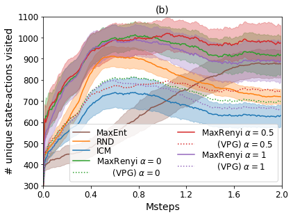
Experiments on MultiRooms. The observation in MultiRooms is the first person perspective from the agent which is high-dimensional and partially observable, and the actions are turning left/right, moving forward and opening the door (cf. Figure 3a above). This environment is hard to explore for standard RL algorithms due to sparse reward. In the exploration phase, the agent has to navigate and open the doors to explore through a series of rooms. In the planning phase, we randomly assign a goal state-action pair, reward the agent upon this state-action, and then train a policy with this reward function. We compare our exploration algorithm MaxRenyi with ICM (Pathak et al. 2017), RND (Burda et al. 2019b) (which use different prediction errors as the intrinsic reward), MaxEnt (Hazan et al. 2019) (which maximizes the state space entropy) and an ablated version of our algorithm MaxRenyi(VPG) (that updates the policy directly by vanilla policy gradient using (2) and (3)).
For the exploration phase, we show the performance of different algorithms in Figure 3b. First, we see that variants of MaxRenyi performs better than the baseline algorithms. Specifically, MaxRenyi is more stable than ICM and RND that explores well at the start but later degenerates when the agent becomes familiar with all the states. Second, we observe that MaxRenyi performs better than MaxRenyi(VPG) with different s, indicating that MaxRenyi benefits from adopting PPO which reduces variance with a value function and update the policy conservatively. Third, MaxRenyi with performs better than which is consistent with our theory. However, we observe that MaxRenyi with is more likely to be unstable empirically and results in slightly worse performance. At last, we show the visitation frequency of the exploratory policies resulted from different algorithms in Figure 3a. We see that MaxRenyi visits the states more uniformly compared with the baseline algorithms, especially the hard-to-reach states such as the corners of the rooms.
For the planning phase, we collect datasets of different sizes by executing different exploratory policies, and use the datasets to compute policies with different reward functions using BCQ. We show the performance of the resultant policies in Figure 3c. First, we observe that the datasets generated by running random policies do not lead to a successful planning, indicating the importance of learning a good exploratory policy in this framework. Second, the dataset with only 8k samples leads to a successful planning (with a normalized cumulative reward larger than 0.8) using MaxRenyi, whereas a dataset with 16k samples is needed to succeed in the planning phase when using ICM, RND or MaxEnt. This illustrates that MaxRenyi leads to a better performance in the planning phase (i.e., attains good policies with fewer samples) than the previous exploration algorithms.
Further, we compare MaxRenyi that maximizes the entropy over the state-action space with two ablated versions: “State + bonus” that maximizes the entropy over the state space with an entropy bonus (i.e., using to estimate the state distribution in Algorithm 1), and “State” that maximizes the entropy over the state space (i.e., additionally setting in (6)). Notice that the reward-free RL framework requires that a good policy is obtained for arbitrary reward functions in the planning phase. Therefore, we show the lowest normalized cumulative reward of the planned policies across different reward functions for the algorithms in Table 1. We see that maximizing the entropy over the state-action space results in better performance for this framework.
| 2k | 4k | 8k | 16k | |
|---|---|---|---|---|
| MaxRenyi | 0.14 | 0.52 | 0.87 | 0.91 |
| State + bonus | 0.14 | 0.48 | 0.78 | 0.87 |
| State | 0.07 | 0.15 | 0.41 | 0.57 |
Experiments on Atari and Mujoco. In the exploration phase, we run different exploration algorithms in the reward-free environment of Atari (Mujoco) for 200M (10M) steps and collect a dataset with 100M (5M) samples by executing the learned policy. In the planning phase, a policy is computed offline to maximize the performance under the extrinsic game reward using the batch RL algorithm based on the dataset. We show the performance of the planned policies in Table 2. We can see that MaxRenyi performs well on a range of tasks with high-dimensional observations or continuous state-actions for the reward-free RL framework.
| MaxRenyi | RND | ICM | Random | |
| Montezuma | 8,100 | 4,740 | 380 | 0 |
| Venture | 900 | 840 | 240 | 0 |
| Gravitar | 1,850 | 1,890 | 940 | 340 |
| PrivateEye | 6,820 | 3,040 | 100 | 100 |
| Solaris | 2,192 | 1,416 | 1,844 | 1,508 |
| Hopper | 973 | 819 | 704 | 78 |
| HalfCheetah | 1,466 | 1,083 | 700 | 54 |
We also provide detailed results for Montezuma’s Revenge and Hopper. For Montezuma’s Revenge, we show the result for the exploration phase in Figure 4a. We observe that although MaxRenyi learns an exploratory policy in a reward-free environment, it achieves reasonable performance under the extrinsic game reward and performs better than RND and ICM. We also provide the number of visited rooms along the training in Appendix Experiment settings, hyperparameters and more experiments., which demonstrates that our algorithm performs better in terms of the state space coverage as well. In the planning phase, we design two different sparse reward functions that only reward the agent if it goes through Room 3 or Room 7 (to the next room). We show the trajectories of the policies planned with the two reward functions in red and blue respectively in Figure 4b. We see that although the reward functions are sparse, the agent chooses the correct path (e.g., opening the correct door in Room 1 with the only key) and successfully reaches the specified room. This indicates that our algorithm generates good policies for different reward functions based on an offline planning in complex environments. For Hopper, we show the t-SNE (Maaten and Hinton 2008) plot of the state-actions randomly sampled from the trajectories generated by different policies in Figure 5. We can see that MaxRenyi generates state-actions that are distributed more uniformly than RND and overlap those from the expert policy. This indicates that the good performance of our algorithm in the planning phase is resulted from the better coverage of our exploratory policy.

6 Conclusion
In this paper, we consider a reward-free RL framework, which is useful when there are multiple reward functions of interest or when we design reward functions offline. In this framework, an exploratory policy is learned by interacting with a reward-free environment in the exploration phase and generates a dataset. In the planning phase, when the reward function is specified, a policy is computed offline to maximize the corresponding cumulative reward using the batch RL algorithm based on the dataset. We propose a novel objective function, the Rényi entropy over the state-action space, for the exploration phase. We theoretically justify this objective and design a practical algorithm to optimize for this objective. In the experiments, we show that our exploration algorithm is effective under this framework, while being more sample efficient and more robust than the previous exploration algorithms.
Acknowledgement
Chuheng Zhang and Jian Li are supported in part by the National Natural Science Foundation of China Grant 61822203, 61772297, 61632016, 61761146003, and the Zhongguancun Haihua Institute for Frontier Information Technology, Turing AI Institute of Nanjing and Xi’an Institute for Interdisciplinary Information Core Technology. Yuanying Cai and Longbo Huang are supported in part by the National Natural Science Foundation of China Grant 61672316, and the Zhongguancun Haihua Institute for Frontier Information Technology, China.
References
- Abdolmaleki et al. (2018) Abdolmaleki, A.; Springenberg, J. T.; Tassa, Y.; Munos, R.; Heess, N.; and Riedmiller, M. 2018. Maximum a posteriori policy optimisation. In Proceedings of the 6th International Conference on Learning Representations.
- Achiam and Sastry (2016) Achiam, J.; and Sastry, S. 2016. Surprise-based intrinsic motivation for deep reinforcement learning. In Deep RL Workshop, Advances in Neural Information Processing Systems.
- Agarwal et al. (2019) Agarwal, A.; Kakade, S. M.; Lee, J. D.; and Mahajan, G. 2019. Optimality and approximation with policy gradient methods in markov decision processes. arXiv preprint arXiv:1908.00261 .
- Auer, Cesa-Bianchi, and Fischer (2002) Auer, P.; Cesa-Bianchi, N.; and Fischer, P. 2002. Finite-time analysis of the multiarmed bandit problem. Machine Learning 47(2-3): 235–256.
- Bellemare et al. (2016) Bellemare, M.; Srinivasan, S.; Ostrovski, G.; Schaul, T.; Saxton, D.; and Munos, R. 2016. Unifying count-based exploration and intrinsic motivation. In Advances in Neural Information Processing Systems, 1471–1479.
- Brockman et al. (2016) Brockman, G.; Cheung, V.; Pettersson, L.; Schneider, J.; Schulman, J.; Tang, J.; and Zaremba, W. 2016. OpenAI Gym.
- Bromiley, Thacker, and Bouhova-Thacker (2004) Bromiley, P.; Thacker, N.; and Bouhova-Thacker, E. 2004. Shannon entropy, Renyi entropy, and information. Statistics and Inf. Series (2004-004) .
- Burda et al. (2019a) Burda, Y.; Edwards, H.; Pathak, D.; Storkey, A.; Darrell, T.; and Efros, A. A. 2019a. Large-scale study of curiosity-driven learning. In Proceedings of the 7th International Conference on Learning Representations.
- Burda et al. (2019b) Burda, Y.; Edwards, H.; Storkey, A.; and Klimov, O. 2019b. Exploration by random network distillation. In Proceedings of the 7th International Conference on Learning Representations.
- Chevalier-Boisvert, Willems, and Pal (2018) Chevalier-Boisvert, M.; Willems, L.; and Pal, S. 2018. Minimalistic Gridworld Environment for OpenAI Gym. https://github.com/maximecb/gym-minigrid.
- Conti et al. (2018) Conti, E.; Madhavan, V.; Such, F. P.; Lehman, J.; Stanley, K.; and Clune, J. 2018. Improving exploration in evolution strategies for deep reinforcement learning via a population of novelty-seeking agents. In Advances in Neural Information Processing Systems, 5027–5038.
- Dann, Lattimore, and Brunskill (2017) Dann, C.; Lattimore, T.; and Brunskill, E. 2017. Unifying PAC and regret: Uniform PAC bounds for episodic reinforcement learning. In Advances in Neural Information Processing Systems, 5713–5723.
- de Abril and Kanai (2018) de Abril, I. M.; and Kanai, R. 2018. Curiosity-driven reinforcement learning with homeostatic regulation. In Proceedings of the International Joint Conference on Neural Networks (IJCNN), 1–6. IEEE.
- Duan et al. (2016) Duan, Y.; Schulman, J.; Chen, X.; Bartlett, P. L.; Sutskever, I.; and Abbeel, P. 2016. RL2: Fast reinforcement learning via slow reinforcement learning. arXiv preprint arXiv:1611.02779 .
- Ecoffet et al. (2019) Ecoffet, A.; Huizinga, J.; Lehman, J.; Stanley, K. O.; and Clune, J. 2019. Go-explore: a new approach for hard-exploration problems. arXiv preprint arXiv:1901.10995 .
- Eysenbach et al. (2019) Eysenbach, B.; Gupta, A.; Ibarz, J.; and Levine, S. 2019. Diversity is all you need: Learning skills without a reward function. In Proceedings of the 7th International Conference on Learning Represention.
- Finn, Abbeel, and Levine (2017) Finn, C.; Abbeel, P.; and Levine, S. 2017. Model-agnostic meta-learning for fast adaptation of deep networks. In Proceedings of the 34th International Conference on Machine Learning, volume 70, 1126–1135. JMLR.
- Flajolet, Gardy, and Thimonier (1992) Flajolet, P.; Gardy, D.; and Thimonier, L. 1992. Birthday paradox, coupon collectors, caching algorithms and self-organizing search. Discrete Applied Mathematics 39(3): 207–229.
- Fujimoto et al. (2019) Fujimoto, S.; Conti, E.; Ghavamzadeh, M.; and Pineau, J. 2019. Benchmarking Batch Deep Reinforcement Learning Algorithms. In Deep RL Workshop, Advances in Neural Information Processing Systems.
- Fujimoto, Meger, and Precup (2019) Fujimoto, S.; Meger, D.; and Precup, D. 2019. Off-Policy Deep Reinforcement Learning without Exploration. In Proceedings of the 36th International Conference on Machine Learning, volume 97, 2052–2062. JMLR.
- Gupta et al. (2018) Gupta, A.; Eysenbach, B.; Finn, C.; and Levine, S. 2018. Unsupervised meta-learning for reinforcement learning. arXiv preprint arXiv:1806.04640 .
- Haarnoja et al. (2017) Haarnoja, T.; Tang, H.; Abbeel, P.; and Levine, S. 2017. Reinforcement learning with deep energy-based policies. In Proceedings of the 34th International Conference on Machine Learning, volume 70, 1352–1361. JMLR.
- Haarnoja et al. (2018) Haarnoja, T.; Zhou, A.; Abbeel, P.; and Levine, S. 2018. Soft actor-critic: Off-policy maximum entropy deep reinforcement learning with a stochastic actor. In Proceedings of the 35th International Conference on Machine Learning, volume 80, 1861–1870. JMLR.
- Hazan et al. (2019) Hazan, E.; Kakade, S.; Singh, K.; and Van Soest, A. 2019. Provably Efficient Maximum Entropy Exploration. In Proceedings of the 36th International Conference on Machine Learning, volume 97, 2681–2691. JMLR.
- Houthooft et al. (2016) Houthooft, R.; Chen, X.; Duan, Y.; Schulman, J.; De Turck, F.; and Abbeel, P. 2016. Vime: Variational information maximizing exploration. In Advances in Neural Information Processing Systems, 1109–1117.
- Islam et al. (2019) Islam, R.; Seraj, R.; Bacon, P.-L.; and Precup, D. 2019. Entropy Regularization with Discounted Future State Distribution in Policy Gradient Methods. In Optimization Foundations of RL Workshop, Advances in Neural Information Processing Systems.
- Jin et al. (2020) Jin, C.; Krishnamurthy, A.; Simchowitz, M.; and Yu, T. 2020. Reward-Free Exploration for Reinforcement Learning. In Proceedings of the 37th International Conference on Machine Learning. JMLR.
- Kingma and Welling (2014) Kingma, D. P.; and Welling, M. 2014. Auto-encoding variational bayes. In Proceedings of the 2nd International Conference on Learning Representations.
- Lai and Robbins (1985) Lai, T. L.; and Robbins, H. 1985. Asymptotically efficient adaptive allocation rules. Advances in Applied Mathematics 6(1): 4–22.
- Lange, Gabel, and Riedmiller (2012) Lange, S.; Gabel, T.; and Riedmiller, M. 2012. Batch reinforcement learning. In Reinforcement learning, 45–73. Springer.
- Lehman and Stanley (2011) Lehman, J.; and Stanley, K. O. 2011. Novelty search and the problem with objectives. In Genetic programming theory and practice IX, 37–56. Springer.
- Maaten and Hinton (2008) Maaten, L. v. d.; and Hinton, G. 2008. Visualizing data using t-SNE. Journal of machine learning research 9(Nov): 2579–2605.
- Machado et al. (2018) Machado, M. C.; Bellemare, M. G.; Talvitie, E.; Veness, J.; Hausknecht, M. J.; and Bowling, M. 2018. Revisiting the Arcade Learning Environment: Evaluation Protocols and Open Problems for General Agents. Journal of Artificial Intelligence Research 61: 523–562.
- Misra et al. (2019) Misra, D.; Henaff, M.; Krishnamurthy, A.; and Langford, J. 2019. Kinematic State Abstraction and Provably Efficient Rich-Observation Reinforcement Learning. arXiv preprint arXiv:1911.05815 .
- Mohamed and Rezende (2015) Mohamed, S.; and Rezende, D. J. 2015. Variational information maximisation for intrinsically motivated reinforcement learning. In Advances in Neural Information Processing Systems, 2125–2133.
- Nachum et al. (2017) Nachum, O.; Norouzi, M.; Xu, K.; and Schuurmans, D. 2017. Bridging the gap between value and policy based reinforcement learning. In Advances in Neural Information Processing Systems, 2775–2785.
- Nagabandi et al. (2019) Nagabandi, A.; Clavera, I.; Liu, S.; Fearing, R. S.; Abbeel, P.; Levine, S.; and Finn, C. 2019. Learning to adapt in dynamic, real-world environments through meta-reinforcement learning. In Proceedings of the 7th International Conference on Learning Representations.
- Ostrovski et al. (2017) Ostrovski, G.; Bellemare, M. G.; van den Oord, A.; and Munos, R. 2017. Count-based exploration with neural density models. In Proceedings of the 34th International Conference on Machine Learning-Volume 70, 2721–2730. JMLR. org.
- Pathak et al. (2017) Pathak, D.; Agrawal, P.; Efros, A. A.; and Darrell, T. 2017. Curiosity-driven exploration by self-supervised prediction. In Proceedings of the IEEE Conference on Computer Vision and Pattern Recognition Workshops, 16–17.
- Puterman (2014) Puterman, M. L. 2014. Markov decision processes: discrete stochastic dynamic programming. John Wiley & Sons.
- Sanei, Borzadaran, and Amini (2016) Sanei, M.; Borzadaran, G. R. M.; and Amini, M. 2016. Renyi entropy in continuous case is not the limit of discrete case. Mathematical Sciences and Applications E-Notes 4.
- Schmidhuber (1991) Schmidhuber, J. 1991. A possibility for implementing curiosity and boredom in model-building neural controllers. In Proceedings of the international conference on simulation of adaptive behavior: From animals to animats, 222–227.
- Schulman, Chen, and Abbeel (2017) Schulman, J.; Chen, X.; and Abbeel, P. 2017. Equivalence between policy gradients and soft q-learning. arXiv preprint arXiv:1704.06440 .
- Schulman et al. (2016) Schulman, J.; Moritz, P.; Levine, S.; Jordan, M.; and Abbeel, P. 2016. High-dimensional continuous control using generalized advantage estimation. In Proceedings of the 4th International Conference of Learning Representations.
- Schulman et al. (2017) Schulman, J.; Wolski, F.; Dhariwal, P.; Radford, A.; and Klimov, O. 2017. Proximal policy optimization algorithms. arXiv preprint arXiv:1707.06347 .
- Silver (2015) Silver, D. 2015. Lecture 2: Markov Decision Processes. UCL. Retrieved from www0. cs. ucl. ac. uk/staff/d. silver/web/Teaching_files/MDP. pdf .
- Strehl and Littman (2008) Strehl, A. L.; and Littman, M. L. 2008. An analysis of model-based interval estimation for Markov decision processes. Journal of Computer and System Sciences 74(8): 1309–1331.
- Sutton and Barto (2018) Sutton, R. S.; and Barto, A. G. 2018. Reinforcement Learning: An Introduction. MIT press Cambridge.
- Todorov, Erez, and Tassa (2012) Todorov, E.; Erez, T.; and Tassa, Y. 2012. Mujoco: A physics engine for model-based control. In 2012 IEEE/RSJ International Conference on Intelligent Robots and Systems, 5026–5033. IEEE.
- Wang et al. (2016) Wang, J. X.; Kurth-Nelson, Z.; Tirumala, D.; Soyer, H.; Leibo, J. Z.; Munos, R.; Blundell, C.; Kumaran, D.; and Botvinick, M. 2016. Learning to reinforcement learn. arXiv preprint arXiv:1611.05763 .
- Williams (1992) Williams, R. J. 1992. Simple statistical gradient-following algorithms for connectionist reinforcement learning. Machine Learning 8(3-4): 229–256.
The toy example in Figure 1
In this example, the initial state is fixed to be . Due to the simplicity of this toy example, we can solve for the policy that maximizes the Rényi entropy of the state-action distribution with and . The optimal policy is
where represents the probability of choosing on . The corresponding state-action distribution is
where the -th element represents the probability density of the state-action distribution on . Using equation (1), we obtain which is the expected number of samples collected form this distribution that contains all the state-action pairs.
An example to illustrate the advantage of using Rényi entropy
Although we did not justify theoretically that Rényi entropy serves as a better surrogate function of than Shannon entropy in the main text, here we illustrate that this may hold in general. Specifically, we try to show that the corresponding of the policy that maximizes Rényi entropy with small is always smaller than that of the policy that maximizes Shannon entropy. Notice that when the dynamics is known to be deterministic, indicates how many samples are needed in expectation to ensure a successful planning. In the stochastic setting, also serves as a good indicator since this is the lower bound of the number of samples needed for a successful planning.
To show that Rényi entropy is a good surrogate function, we can use brute-force search to check if there exists a CMP on which the Shannon entropy is better than Rényi entropy in terms of . As an illustration, we only consider CMPs with two states and two actions. Specifically, for this family of CMPs, there are 5 free parameters to be searched: 4 parameters for the transition dynamics and 1 parameter for the initial state distribution. We set step size for searching to 0.1 for each parameter and use , . The result shows there does not exists any CMP on which the Shannon entropy is better than Rényi entropy in term of out of the searched CMPs.
To further investigate, we consider a specific CMP. The transition matrix of this CMP is
where the rows corresponds to respectively and the columns corresponds the next states ( and respectively). The initial state distribution of this CMP is
For this CMP, the value of the policy that maximizes Shannon entropy is 88, while the values are only 39 and 47 for policies that maximize Rényi entropy with , respectively. The optimal value is 32. This indicates that we may need 2x more samples to accurately estimate the dynamics of the CMP. We observe is much harder to reach than on this CMP: The initial state is always and taking action will always reach . In order to visit more, policies should take with a high probability on . In fact, the policy that maximizes Shannon entropy takes on with the probability of only 0.58, while the policies that maximize Rényi entropy with and take on with probabilities 0.71 and 0.64 respectively.
This example illustrates the following essence that widely exists in other CMPs: A good objective function should encourage the policy to visit the hard-to-reach state-actions as frequently as possible and Rényi entropy does a better job than Shannon entropy from this perspective.
Proof of Theorem 3.1
We provide Theorem 3.1 to justify our objective that maximizes the entropy over the state-action space in the exploration phase for the reward-free RL framework. In the following analysis, we consider the standard episodic and tabular case as follows: The MDP is defined as , where is the state space with , is the action space with , is the length of each episode, is the set of unknown transition matrices, is the set of the reward functions and is the unknown initial state distribution. We denote as the transition probability from to on the -th step. We assume that the instant reward for taking the action on the state on the -th step is deterministic. A policy specifies the probability of choosing the actions on each state and on each step. We denote the set of all such policies as .
The agent with policy interacts with the MDP as follows: At the start of each episode, an initial state is sampled from the distribution . Next, at each step , the agent first observes the state and then selects an action from the distribution . The environment returns the reward and transits to the next state according to the probability . The state-action distribution induced by on the -th step is .
The state value function for a policy is defined as . The objective is to find a policy that maximizes the cumulative reward .
The proof goes through in a similar way to that of Jin et al. (2020).
Input: A dataset of transitions ; The reward function ; The level of accuracy .
Proof of Theorem 3.1.
Given the dataset specified in the theorem, a reward function and the level of accuracy , we use the planning algorithm shown in Algorithm 2 to obtain a near-optimal policy . The planning algorithm first estimates a transition matrix based on and then solves for a policy based on the estimated transition matrix and the reward function .
Define and is the value function on the MDP with the transition dynamics . We first decompose the error into the following terms:
Then, the proof of the theorem goes as follows:
To bound the two evaluation error terms, we first present Lemma .4 to show that the policy which maximizes Rényi entropy is able to visit the state-action space reasonably uniformly, by leveraging the convexity of the feasible region in the state-action distribution space (Lemma .2). Then, with Lemma .4 and the concentration inequality Lemma .5, we show that the two evaluation error terms can be bounded by for any policy and any reward function (Lemma .7).
To bound the optimization error term, we use the natural policy gradient (NPG) algorithm as the APPROXIMATE-MDP-SOLVER in Algorithm 2 to solve for a near-optimal policy on the estimated and the given reward function . Finally, we apply the optimization bound for the NPG algorithm (Agarwal et al. 2019) to bound the optimization error term (Lemma .8).
∎
Definition .1 ().
is defined as the feasible region in the state-action distribution space , , where is the cardinality of the state-action space.
Hazan et al. (Hazan et al. 2019) proved the convexity of such feasible regions in the infinite-horizon and discounted setting. For completeness, we provide a similar proof on the convexity of in the episodic setting.
Lemma .2.
[Convexity of ] is convex. Namely, for any and , denote and , there exists a policy such that .
Proof of Lemma .2.
Define a mixture policy that first chooses from with probability and respectively at the start of each episode, and then executes the chosen policy through the episode. Define the state distribution (or the state-action distribution) for this mixture policy on each layer as . Obviously, . For any mixture policy , we can construct a policy where such that (Puterman 2014). In this way, we find a policy such that . ∎
Similar to Jin et al. (Jin et al. 2020), we define -significance for state-action pairs on each step and show that the policy that maximizes Rényi entropy is able to reasonably uniformly visit the significant state-action pairs.
Definition .3 (-significance).
A state-action pair on the -th step is -significant if there exists a policy , such that the probability to reach following the policy is greater than , i.e., .
Recall the way we construct the dataset : With the set of policies where and , we first uniformly randomly choose a policy from at the start of each episode, and then execute the policy through the episode. Note that there is a set of policies that maximize the Rényi entropy on the -th layer since the policy on the subsequent layers does not affect the entropy on the -th layer. We denote the induced state-action distribution on the -th step as , i.e., the dataset can be regarded as being sampled from for each step . Therefore, .
Lemma .4.
If , then
| (7) |
Proof of Lemma .4.
For any -significant , consider the policy . Denote . We can treat as a vector with dimensions and use the first dimension to represent , i.e., . Denote . Since , . By Lemma .2, . Since is concave over when , will monotonically increase as we increase from 0 to , i.e.,
This is true when , i.e., when , we have
Since are non-negative, we have
Note that , we have
| (8) |
Since , we have . Using the fact that , we can obtain the inequality in (7). ∎
When , we have
When ,
Lemma .5.
Suppose is the empirical transition matrix estimated from samples that are i.i.d. drawn from and is the true transition matrix, then with probability at least , for any and any value function , we have:
| (9) |
Proof of Lemma .5.
The lemma is proved in a similar way to that of Lemma C.2 in (Jin et al. 2020) that uses a concentration inequality and a union bound. The proof differs in that we do not need to count the different events on the action space for the union bound since the state-action distribution is given here (instead of only the state distribution). This results in a missing factor in the logarithm term compared with their lemma. ∎
Lemma .6 (Lemma E.15 in Dann et al. (Dann, Lattimore, and Brunskill 2017)).
For any two MDPs and with rewards and and transition probabilities and , the difference in values and with respect to the same policy is
Lemma .7.
Under the conditions of Theorem 3.1, with probability at least , for any reward function and any policy , we have:
| (10) |
Proof of Lemma .7.
The proof is similar to Lemma 3.6 in Jin et al. (Jin et al. 2020) but differs in several details. Therefore, we still provide the proof for completeness. The proof is based on the following observations: 1) The total contribution of all insignificant state-action pairs is small; 2) is reasonably accurate for significant state-action pairs due to the concentration inequality in Lemma .5.
Using Lemma .6 on and with the true transition dynamics and the estimated transition dynamics respectively, we have
Let be the set of -significant state-action pairs on the -th step. We have
By the definition of -significant pairs, we have
As for , by Cauchy-Shwartz inequality and Lemma .4, we have
By Lemma .5, we have
Thus, we have
Therefore, combining inequalities above, we have
where and . With , it is sufficient to ensure that , if we set
Especially, for , we have
To establish (10), we can choose and set for sufficiently large absolute constant . ∎
We use the natural policy gradient (NPG) algorithm as the approximate MDP solver.
Policy gradient of state-action space entropy
In the following derivation, we use the notation that sums over the states or the state-action pairs. Nevertheless, it can be easily extended to continuous state-action spaces by simply replacing summation by integration. Note that, although the Rényi entropy for continuous distributions is not the limit of the Rényi entropy for discrete distributions (since they differs by a constant (Sanei, Borzadaran, and Amini 2016)), their gradients share the same form. Therefore, the derivation still holds for the continuous case.
Lemma .1 (Gradient of discounted state visitation distribution).
A policy is parameterized by . The gradient of the discounted state visitation distribution induced by the policy w.r.t. the parameter is
| (12) |
Proof.
The discounted state visitation distribution started from one state-action pair can be written as the distribution started from the next state-action pair.
where .
Then, the proof follows an unrolling procedure on the discounted state visitation distribution as follows:
At last,
∎
Lemma .2 (Policy gradient of the Shannon entropy over the state-action space).
Given a policy parameterized by , the gradient of w.r.t. the parameter is as follows:
| (13) |
Proof.
First, we can calculate the gradient of Shannon entropy where is the state-action distribution and is a normalization factor. Then, we observe that .
Using the standard chain rule and Lemma .1, we can obtain the policy gradient:
where is the cross-entropy between the two distributions. We use the fact in the first line. ∎
Lemma .3 (Policy gradient of the Rényi entropy over the state-action space).
Given a policy parameterized by and , the gradient of w.r.t. the parameter is as follows:
| (14) |
Proof.
First, we note that the gradient of Rényi entropy is
where is a constant normalizer. Given a vector and a real number , we use to denote the vector . Similarly, using the chain rule and Lemma .1, we have
∎
We should note that when , ; and when , . Especially, we can write down the case for :
| (15) |
This leads to a policy gradient update with reward . This inverse-square-root style reward is frequently used as the exploration bonus in standard RL problems (Strehl and Littman 2008; Bellemare et al. 2016) and similar to the UCB algorithm (Auer, Cesa-Bianchi, and Fischer 2002; Lai and Robbins 1985) in the bandit problem.
Practical implementation
Recall the deduced policy gradient formulations of the entropies on a CMP in (13) and (14). We observe that if we set the reward function (when ) or (when ), these policy gradient formulations can be compared with the policy gradient for a standard MDP: The first term resembles the policy gradient of cumulative reward and the second term resembles the policy gradient of instant reward .
For the first term, a wide range of existing policy gradient based algorithms can be used to estimate this term. Since these algorithms such as PPO do not retain the scale of the policy gradient, we induce a coefficient to adjust for the scale between this term and the second term.
For the second term, when , this term can be reduced to
where denotes the Shannon entropy over the action distribution conditioned on the state sample . Although the two sides are equivalent in expectation, the right hand side leads to smaller variance when estimated using samples due to the following reasons: First, the left hand side is calculated with the values of a density estimator (that estimates ) on the state-action samples and the density estimator suffers from high variance. In contrast, the right hand side does not involve the density estimation. Second, to estimate the expectation with samples, the left hand side uses both the state samples and the action samples while the right hand side uses only the state samples and the action distributions conditioned on these states. This reduces the variance in the estimation. When , since the second term in equation (2) can hardly be reduced to such a simple form, we still use as the approximation.
Value function estimator
In this section, we provide the detail of the truncated TD() estimator (Sutton and Barto 2018) that we use in our algorithm. Recall that in the -th iteration, we maintain the replay buffer as where is the length of the -th trajectory and is the total number of trajectories in the replay buffer. Correspondingly, the reward calculated using the latest density estimator is denoted as or for each , .
The truncated n-step value function estimator can be written as:
where is the current value function network with the parameter . Notice that, since the discount rate is considered when we collect sample, here we estimate the undiscounted sum. When (i.e., ), this corresponds to the Monte Carlo estimator whose variance is high. When (i.e., ), this corresponds to the TD(0) estimator that has large bias. To balance variance and bias, we use the truncated TD() estimator which is the weighted sum of the truncated n-step estimators with different , i.e.,
where and are the hyperparameters.
Experiment settings, hyperparameters and more experiments.
.1 Experiment settings and hyperparameters
Throughout the experiments, we set the hyperparameters as follows: The coefficient that balances the two terms in the policy gradient formulation is . The parameter for computing GAE and the target state values is . The steps for computing the target state values is . The learning rate for the policy network is and the learning rate for VAE and the value function .
In Pendulum and FourRooms (see Appendix .2), we use and store samples of the latest 10 iterations in the replay buffer. To estimate the corresponding Rényi entropy of the policy during the training in the top of Figure 6, we sample several trajectories in each iteration. In each trajectory, we terminate the trajectory on each step with probability . For and , we sample 1000 trajectories to estimate the distribution and then calculate the Rényi entropy over the state-action space. For , we sample 50 groups of trajectories. In the -th group, we sample 20 trajectories and count the number of unique state-action pairs visited . We use as the estimation of the Rényi entropy when . The corresponding entropy of the optimal policy is estimated in a same manner. The bottom figures in Figure 6 is plotted using 100 trajectories, each of which is also collected in a same manner.
In MultiRooms, we use and store samples of the latest 10 iterations in the replay buffer. We use the MiniGrid-MultiRoom-N6-v0 task from minigrid. We fix the room configuration for a single run of the algorithm and use different room configurations in different runs. The four actions are turning left/right, moving forward and opening the door. In the planning phase, we randomly pick grids and construct the corresponding reward functions. The reward function gives the agent a reward if the agent reaches the corresponding state and gives a reward otherwise. We show the means and the standard deviations of five runs with different random seeds in the figures.
For Atari games, we use and store samples of the latest 20 iterations in the replay buffer. For Mujoco tasks, we use and only store samples of the current iteration. In Figure 4b, the two reward functions in the planning phase are designed as follows: Assume the rooms are numbered in the default order by the environment (cf. the labels in Figure 4b). Under the first reward function, when the agent goes from Room 3 to Room 9 (the room below Room 3) for the first time, we assign a unit reward to the agent. Otherwise, we assign zero rewards to the agent. Similarly, under the second reward function, we give a reward to the agent when it goes from Room 7 to Room 13 (the room below Room 7).
We will release the source code for this experiments once the paper is published.
.2 Convergence of MaxRenyi
Convergence is one of the most critical properties of an algorithm. The algorithm based on maximizing Shannon entropy has a convergence guarantee leveraging the existing results on the convergence of standard RL algorithms and its similar form to the standard RL problem (noting that and ) (Hazan et al. 2019). On the other hand, MaxRenyi does not have such a guarantee not only due to the form of Rényi entropy but also due to the techniques we use. Therefore, we present a set of experiments here to illustrate whether our exploration algorithm MaxRenyi empirically converges to near-optimal policies in terms of the entropy over the state-action space. To answer this question, we compare the entropy induced by the agent during the training in MaxRenyi with the maximum entropy the agent can achieve. We implement MaxRenyi for two simple environments, Pendulum and FourRooms, where we can solve for the maximum entropy by brute force search. Pendulum from OpenAI Gym (Brockman et al. 2016) has a continuous state-action space. For this task, the entropy is estimated by discretizing the state space into grids and the action space into two discrete actions. FourRooms is a grid world environment with four actions and deterministic transitions. We show the results in Figure 6. The results indicate that our exploration algorithm approaches the optimal in terms of the corresponding state-action space entropy with different in both discrete and continuous settings.


.3 More results for Atari games and Mujoco tasks
The reward-free RL framework contains two phases, the exploration phase and the planning phase. Due to space limit, we only show the final performance of the algorithms (i.e., the performance of the agent planned based on the data collected using the learned exploratory policy) in the main text. Here, we also show the performance of the exploration algorithms in the exploration phase (i.e., the performance for the reward-free exploration setting). We show the results in Table 3. First, the scores for the exploration phase are measured using the extrinsic game rewards of the tasks. However, the exploration algorithms are trained in the reward-free exploration setting (i.e., do not receive such extrinsic game rewards). The results indicate that, although MaxRenyi is designed for the reward-free RL framework, it outperforms other exploration algorithms in the reward-free exploration setting. Then, the average scores for the planning phase is the same as those in Table 1. In addition, we present the standard deviations over five random seeds. The results indicate that the stability of MaxRenyi is comparable to RND and ICM while achieving better performance on average.
| MaxRenyi | RND | ICM | Random | ||
|---|---|---|---|---|---|
| Exploration phase | Montezuma | 7,540(2210) | 4,220(736) | 1,140(1232) | 0 |
| Venture | 460(273) | 740(546) | 120(147) | 0 | |
| Gravitar | 1,420(627) | 1,010(886) | 580(621) | 173 | |
| PrivateEye | 6,480(7,813) | 6,220(7,505) | 100(0) | 25 | |
| Solaris | 1,284(961) | 1,276(712) | 1,136(928) | 1,236 | |
| Hopper | 207(628) | 72(92) | 86(75) | 31 | |
| HalfCheetah | 456(328) | 137(126) | 184(294) | -82 | |
| Planning phase | Montezuma | 8,100(1,124) | 4,740(2,216) | 380(146) | 0(0) |
| Venture | 900(228) | 840(307) | 240(80) | 0(0) | |
| Gravitar | 1,850(579) | 1,890(665) | 940(281) | 340(177) | |
| PrivateEye | 6,820(7,058) | 3,040(5,880) | 100(0) | 100(0) | |
| Solaris | 2,192(1,547) | 1,416(734) | 1,844(173) | 1,508(519) | |
| Hopper | 973(159) | 819(87) | 704(59) | 78(36) | |
| HalfCheetah | 1,466(216) | 1,083(377) | 700(488) | 54(50) |
.4 More results for Montezuma’s Revenge
Although the extrinsic game reward in Montezuma’s Revenge aligns with the coverage of the state space, the number of rooms visited in one episode may be a more direct measure for an exploration algorithm. Therefore, we also provide the curves for the number of rooms visited during the reward-free exploration. Compared with Figure 4a, we observe that, although MaxRenyi visits only slightly more rooms than RND, it yields higher returns by visiting more scoring states. This is possibly because our algorithm encourages the agent to visit the hard-to-reach states more.

Moreover, our algorithm is less likely to fail under different reward functions in the planning phase. There is a failure mode for the planning phase in Montezuma’s Revenge: For example, with the reward to go across Room 3, the trained agent may first go to Room 7 to obtain an extra key and then return to open the door toward Room 0, which is not the shortest path. Out of 5 runs, our algorithms fail 2 times where RND fails all the 5 times.