Exploration and Anti-Exploration with Distributional Random Network Distillation
Abstract
Exploration remains a critical issue in deep reinforcement learning for an agent to attain high returns in unknown environments. Although the prevailing exploration Random Network Distillation (RND) algorithm has been demonstrated to be effective in numerous environments, it often needs more discriminative power in bonus allocation. This paper highlights the “bonus inconsistency” issue within RND, pinpointing its primary limitation. To address this issue, we introduce the Distributional RND (DRND), a derivative of the RND. DRND enhances the exploration process by distilling a distribution of random networks and implicitly incorporating pseudo counts to improve the precision of bonus allocation. This refinement encourages agents to engage in more extensive exploration. Our method effectively mitigates the inconsistency issue without introducing significant computational overhead. Both theoretical analysis and experimental results demonstrate the superiority of our approach over the original RND algorithm. Our method excels in challenging online exploration scenarios and effectively serves as an anti-exploration mechanism in D4RL offline tasks. Our code is publicly available at https://github.com/yk7333/DRND.
1 Introduction
Exploration is a pivotal consideration in reinforcement learning, especially when dealing with environments that offer sparse or intricate reward information. Several methods have been proposed to promote deep exploration (Osband et al., 2016), including count-based and curiosity-driven approaches. Count-based techniques in environments with constrained state spaces rely on recording state visitation frequencies to allocate exploration bonuses (Strehl & Littman, 2008; Azar et al., 2017). However, this method encounters challenges in massive or continuous state spaces. In expansive state spaces, “pseudo counts” have been introduced as an alternative (Bellemare et al., 2016; Lobel et al., 2023; Ostrovski et al., 2017; Machado et al., 2020). However, establishing a correlation between counts and probability density requires rigorous criteria (Ostrovski et al., 2017), complicating the implementation of density-based pseudo counts resulting in a significant dependency on network design and hyperparameters.
Curiosity-driven methods motivate agents to explore and learn by leveraging intrinsic motivation. This inherent motivation, often called “curiosity”, pushes the agent to explore unfamiliar states or actions. Certain approaches derive intrinsic rewards from the prediction loss of environmental dynamics (Achiam & Sastry, 2017; Burda et al., 2018a; Pathak et al., 2017). As states and actions become more familiar, these methods become more efficient. However, these methods can face difficulties when essential information is missing or the target function is inherently stochastic, as highlighted by the “noisy-TV” problem (Pathak et al., 2017). The Random Network Distillation (RND) method uses the matching loss of two networks for a particular state to be the intrinsic motivation (Burda et al., 2018a). It leverages a randomly initialized target network to generate a fixed value for specific states and trains a prediction network to match this output. RND has demonstrated remarkable results in exploration-demanding environments with sparse rewards, such as Montezuma’s Revenge. However, RND has its limitations. While its reliance on network loss for intrinsic rewards lacks a robust mathematical foundation, its interpretability should be more evident compared to count-based techniques. Moreover, the RND method grapples with the issue of bonus inconsistency, which becomes apparent during the initial stages of training when no states have been encountered, leading to bonuses that exhibit considerable deviations from a random distribution. RND struggles to precisely represent the dataset’s distribution as training progresses, resulting in indistinguishable bonuses.
We introduce the Distributional Random Network Distillation (DRND) approach to tackle the challenge of bonus inconsistency in RND. In contrast to the RND method, our approach employs a predictor network to distill multiple random target networks. Our findings demonstrate that the DRND predictor effectively operates as a pseudo-count model. This unique characteristic allows DRND to seamlessly merge the advantages of count-based techniques with the RND method, thereby enhancing performance without incurring additional computational and spatial overheads, as the target networks remain fixed and do not require updates. The curiosity-driven RND method and the pseudo-count Coin Flip Network (CFN, (Lobel et al., 2023)) method are special cases of our DRND method. Through theoretical analysis and an initial experiment (see Section 5.1), we validate that, compared to RND, DRND demonstrates improved resilience to variations in initial state values, provides a more accurate estimate of state transition frequencies, and better discriminates dataset distributions. As a result, DRND outperforms RND by providing better intrinsic rewards.
In online experiments, we combine the DRND method with Proximal Policy Optimization (PPO, (Schulman et al., 2017)). On the image-based exploration benchmark environments Montezuma’s Revenge, Gravitar, and Venture, DRND outperforms baseline PPO, RND, pseudo-count method CFN, and curiosity-driven method ICM (Pathak et al., 2017). In continuous-control gym-robotics environments, our method also outperforms existing approaches. Furthermore, we demonstrate that DRND can also serve as a good anti-exploration penalty term in the offline setting, confirming its ability to provide a better bonus based on the dataset distribution. We follow the setting of SAC-RND (Nikulin et al., 2023) and propose a novel offline RL algorithm, SAC-DRND. We run experiments in D4RL (Fu et al., 2020) offline tasks and find that SAC-DRND outperforms many recent strong baselines across various D4RL locomotion and Antmaze datasets.

2 Related Work
Count-based exploration. Count-based exploration is a strategy in RL where an agent uses count information to guide its exploration of unknown environments. By keeping track of counts for different states or actions, the agent can estimate the level of unknowns associated with each state or action, prioritizing exploration of those with high unknowns (Bellemare et al., 2016; Machado et al., 2020; Martin et al., 2017; Tang et al., 2017). These approaches use or , aiming to balance exploration and exploitation in stochastic MDPs (Strehl & Littman, 2008). Various methods, including CTS (Bellemare et al., 2016), PixelCNN (Ostrovski et al., 2017), Successor Counts (Machado et al., 2020), and CFN (Lobel et al., 2023), have explored calculating pseudocounts in large state spaces to approximate . Furthermore, count-based techniques (Kim & Oh, 2023; Hong et al., 2022) are employed in offline RL to do anti-exploration. While effective in finite state spaces, these methods heavily rely on the network’s ability to approximate probability density functions in large state spaces. Accurately estimating density requires a significant number of samples, which limits the effectiveness of counting methods in situations with small sample sizes or regions of low probability density.
Curiosity-driven exploration. In curiosity-driven methods, the agent’s motivation stems from intrinsic curiosity, often quantified using information-theoretic or novelty-based metrics. One widely used metric involves employing a dynamic model to predict the difference between the expected and actual states, serving as the intrinsic reward (Stadie et al., 2015; Achiam & Sastry, 2017; Pathak et al., 2017), which helps identify unfamiliar patterns, encouraging exploration in less familiar areas. Alternatively, some approaches use information gain as an intrinsic reward (Still & Precup, 2012; Houthooft et al., 2016). Still, they demand computationally intensive network fitting and can struggle in highly stochastic environments due to the “noise TV” problem (Burda et al., 2018b).
Another curiosity-driven method is RND (Burda et al., 2018b), which is a prominent RL exploration baseline. RND employs two neural networks: a static prior and a trainable predictor. Both networks map states to embeddings, with state novelty assessed based on their prediction error, which serves as an exploration bonus. This simplicity has bolstered RND’s popularity in exploration algorithms and demonstrated its potential in supervised settings, even suggesting its use as an ensemble alternative for estimating epistemic uncertainty (Ciosek et al., 2019; Kuznetsov et al., 2020). However, common practices, such as using identical architectures for both networks and estimating novelty solely from states, can result in substantial inconsistencies in reward bonuses.
Anti-Exploration in Model-free Offline RL Offline RL addresses the problem of learning policies from a logged static dataset. Model-free offline algorithms do not require an estimated model and focus on correcting the extrapolation error (Fujimoto et al., 2019) in the off-policy algorithms. The first category emphasizes regularizing the learned policy to align with the behavior policy (Kostrikov et al., 2021; Wang et al., 2018, 2020; Wu et al., 2019; Xie et al., 2021; Fujimoto & Gu, 2021). The second category aims to prevent the OOD actions by modifying the value function (Kumar et al., 2020; Lyu et al., 2023, 2022b; An et al., 2021; Ghasemipour et al., 2022; Yang et al., 2022). These methods employ dual penalization techniques in actor-critic algorithms to facilitate effective offline RL policy learning. These approaches can be further categorized into ensemble-free methods and ensemble-based methods. The ensemble-based methods quantify the uncertainty with ensemble techniques to obtain a robust value function, such as SAC-N (An et al., 2021) and RORL (Yang et al., 2022). The ensemble-free methods adapt conservatism to a value function instead of many value functions (Kumar et al., 2020; Lyu et al., 2022b; Rezaeifar et al., 2022). These methods require punishment for states and actions outside of the dataset distribution, which is called an “anti-exploration” bonus (Rezaeifar et al., 2022) for the agent. Unlike online RL, where novelty bonuses incentivize exploration, offline RL leans towards conservatism, aiming to reduce rewards in uncharted scenarios. In this work, we introduce a distributional random network distillation approach to serve as a novel anti-exploration method, demonstrating the efficacy of SAC-DRND across various offline RL datasets.
3 Preliminaries
MDP. We base our framework on the conventional Markov Decision Process (MDP) formulation as described in (Sutton et al., 1998). In this setting, an agent perceives an observation and executes an action . The transition probability function, denoted by , governs the progression from the current state to the subsequent state upon the agent’s action . Concurrently, the agent is awarded a reward , determined by the reward function . The agent’s objective is to ascertain a policy that optimizes the anticipated cumulative discounted returns, represented as , where serves as the discount factor.


Intrinsic reward. To enhance exploration, a common approach involves augmenting the agent’s rewards in the environment with intrinsic rewards as a bonus. These intrinsic rewards, denoted as , incentivize agents to explore unfamiliar states and take unfamiliar actions. In offline RL, the intrinsic reward is an anti-exploration penalty term to discourage OOD actions. Upon incorporating the intrinsic reward into the original target of the Q value function, the adjusted target can be expressed as follows:
where is the scale of the bonus for the update of the value network.
4 Method
The RND method utilizes two neural networks: a fixed, randomly initialized target network , and a predictor network trained on agent-collected data, where is the observation space. In this section, we highlight RND’s primary issue and introduce our method, Distributional Random Network Distillation (DRND).
4.1 Bonus Inconsistencies in Random Network Distillation
The RND method faces challenges with bonus inconsistencies, which can be categorized into initial and final bonus inconsistencies. The initial bonus inconsistency relates to the uneven distribution of bonuses among states at the beginning of training. Addressing this issue is crucial to preventing significant bonus value disparities among states. Conversely, the final bonus inconsistency arises when the final bonuses do not align with the dataset distribution, making it hard for the agent to effectively distinguish between frequently visited states and those encountered relatively fewer times. This issue becomes particularly pronounced after substantial updates to the predictor network, which hinders the agent’s ability to engage in deep exploration. This issue is depicted in Figure 1.
To tackle this, we introduce a method that distills a random distribution, enhancing performance with minimal computational overhead and addressing the bonus inconsistency challenges.
4.2 Distill the target network of random distribution

Unlike RND, which only has one target network , the DRND algorithm has target networks , which are from a random distribution with randomly initialized parameters and do not participate in training. In DRND, we use as input in the online setting and pair as input in the offline setting. For simplicity, we define (offline setting) or (online setting). For each state-action pair , we construct a variable that satisfies the distribution:
For simplicity, we use some symbols to record the moments of the distribution:
| (1) | ||||
| (2) |
Each time occurs, is sampled from this distribution. We use a predictive network to learn the variable , although using a fixed network to learn a random variable is impossible. We use the MSE loss function to force to align with and the loss is
| (3) |
By minimizing the loss, the optimal when the state-action pair appears times is
| (4) |
where is defined as at the - occurrence of state . For RND, the more times the predictor network is trained in the same state, the closer the output of the target network is. Therefore, directly using loss as a bonus encourages agents to explore new states. The bonus of our method is not equal to the loss since the loss of random variable fitting is unstable. The expected value of the prediction net is given by
| (5) |
where is the count of occurrences of . After multiple training iterations, this value approaches the mean of the target network distribution. Hence, to measure the deviation from this mean, the first bonus of DRND is defined as
| (6) |
Compared to predicting the output of one target net, predicting the mean of multiple networks is equivalent to passing through a high-pass filter on the output of multiple networks, which can avoid the problem of initial bonus inconsistency due to extreme values in one network. Especially if the network is linear, this bonus inconsistency can be quantitatively calculated.
Lemma 4.1.
Let and be i.i.d. samples from . Given the linear model , the expected mean squared error is
| (7) |
where is the variance of .
The complete proof can be seen in Appendix A.1 . Lemma 4.1 shows that if the predictor parameters and target parameters are sampled from the same distribution, the expectation of the first bonus is a function of input .
Lemma 4.2.
Under the assumptions of Lemma 4.1, let , . The bonus difference of and is .
Proof Sketch.
When , the variance of is a constant . The right side of Equation 7 can be rewritten as . So the bonus difference of and is . ∎
| Metrics | RND | DRND |
|---|---|---|
| (Before training) | 0.03770.0248 | 0.00700.0063 |
| (After training) | 0.09460.0409 | 0.04760.0389 |
| Metrics | |||
|---|---|---|---|
| (Before training) | 0.00670.0035 | 0.00700.0038 | 0.01040.0055 |
| (After training) | 0.05240.0248 | 0.07030.0404 | 0.03960.0209 |
Lemma 4.2 suggests that when the input is confined to a bounded interval, and when Equation 6 is utilized to calculate the initial bonus, the expected maximal difference is modulated by the number of target networks. Importantly, this anticipated discrepancy tends to decrease as increases. This observation substantiates that our DRND method, equipped with target networks, exhibits lower bonus inconsistency under a uniform distribution than the RND method, which uses only a single target network.
However, it is essential to note that the network fitting loss determines this bonus. Consequently, it cannot distinguish between states visited multiple times, which stands in contrast to count-based and pseudo-count methods, which do not address the issue of final bonus inconsistency.


4.3 The DRND predictor is secretly a pseudo-count model
It is essential to track data occurrence frequencies to address inconsistent final bonuses. Traditional count-based methods use large tables to record state visitations, while pseudo-count strategies use neural networks for estimation, providing a scalable insight into state visits. However, these methods introduce computational and storage complexities, particularly when dealing with high-dimensional inputs. We constructed a statistic that indirectly estimates state occurrences without extra auxiliary functions.
Lemma 4.3.
Let be the optimal function which satisfy Equation 4, the statistic
| (8) |
is an unbiased estimator of with consistency.
The complete proof can be found in Appendix A.2. Lemma 4.3 shows that when is large, this statistic can effectively recover the number of occurrences of the state , thus implicitly recording the number of occurrences of the state like the pseudo-count method. By minimizing Equation 3 can make and infinitely close, so we replace in with and approximately assume that they are equal. The DRND predictor potentially stores in its weights how much of each state vector is present in the dataset. To correspond to of the count-based method, the second bonus of the DRND agent is
| (9) |
which is the estimation of .
4.4 Bonus of the DRND agent
The total bonus that combines Equations 6 and 9 gives
| (10) |
where represents the scaling factor for the two bonus terms. Figure 2 shows the diagram of our method and the RND method. For smaller values of , the variance of the second bonus estimate is substantial, rendering the first bonus a more dependable measure for states with infrequent occurrences. Conversely, as increases, the variance of the second bonus approaches zero, enhancing its reliability. From the experiments, we found that during the initial training phase, the magnitudes of the two bonuses, denoted as and , are nearly the same. However, as training progresses, the rate at which the first bonus decreases is much faster than that of the second bonus . Eventually, the magnitude of becomes approximately two orders of magnitude lower than . Therefore, if we want to dominate during the early stages of training and have dominate during the later stages, we do not need to set a dynamic coefficient to achieve this functionality. Instead, we can simply set it as a fixed constant . The distribution of various bonuses as well as the total bonus of the DRND method before and after training can be seen in Figure 3.
The aforementioned heatmap serves as a qualitative illustration. We now provide quantitative experimental results to demonstrate that DRND offers superior bonuses compared to RND. In count-based exploration methods, it is common to assess the rationality of the bonus distribution by comparing it with the distribution, where represents the state visitation count. We evaluate the discrepancy between the intrinsic reward distribution and the uniform distribution before training, and the distribution of after training using KL divergence. We randomly select 100 initial dataset distributions and report the mean and variance of the KL divergence. This assessment is denoted as and , where represents the distribution of RND bonus or DRND bonus. The results obtained are presented in Table 1. It is evident that the KL divergence between the bonuses of DRND and the uniform distribution is smaller during the initial training stages, effectively promoting uniform exploration by the agent. In the later stages of training, DRND better aligns with the distribution of , thereby facilitating deeper exploration by the agent.
To validate that gives better and more uniform bonuses during the early stages of training, while better captures the state visitation count later on, we similarly measure the KL divergence between each bonus term , , the overall bonus and (a) the uniform distribution before training; (b) the distribution of after training. The results are presented in Table 2.
From the table, it can be observed that in the early stages of training, performs better, providing a better solution to the initial bonus inconsistency. Conversely, in the later stages of training, performs better, addressing the final bonus inconsistency more effectively. Moreover, from the KL divergence of the total bonus, it is evident that setting a fixed value for achieves the desired effect of having dominate during the early stages and dominate during the later stages, without the need for dynamic adjustments.
The combination of and depends on the environment and task at hand. In some environments, may be more crucial, while in others, the contribution of might be greater. However, regardless of the specifics, properly integrating both can lead to improved performance.
4.5 Connections between DRND and prior methods
The target network of the DRND method remains static throughout the training process. Moreover, its loss and intrinsic reward computations do not entail additional backpropagation steps, thereby maintaining computational efficiency comparable to that of the RND algorithm. Specifically, when the hyperparameters and are set to 1, the expressions for the loss and intrinsic reward become simplified to , which coincides with the formulation utilized in the RND framework. In contrast to count-based and pseudo-count methods, we forgo the utilization of an additional network or table to track state occurrences. Instead, we estimate these occurrences using the statistical information derived from the prediction network itself. When is set to 0 and follows the distribution , the expressions for the loss and intrinsic reward are simplified to and , which align with the pseudo-count approach CFN.


5 Experiment
In this section, we provide empirical evaluations of DRND. Initially, we demonstrate that DRND offers a better bonus than RND, both before and after training. Our online experiments reveal that DRND surpasses numerous baselines, achieving the best results in exploration-intensive environments. In the offline setting, we use DRND as an anti-exploration penalty term and propose the SAC-DRND algorithm, which beats strong baselines in many D4RL datasets.
5.1 Bonus prediction comparison
In this sub-section, we introduce our inconsistency experiments to compare bonus predictions for both RND and DRND. We created a mini-dataset resembling those used in offline RL or online RL replay buffers in the experiments. This small dataset contains data categories labeled from to , with each data type occurring times proportional to its label. Each data point is represented as a one-hot vector with dimensions, where is set to 100. We train both the RND and DRND networks on the dataset and record both the initial intrinsic reward and the final intrinsic reward.
The left panel in Figure 4 illustrates the difference in initial intrinsic rewards between RND and DRND, with the x-axis representing the number of target networks. As increases, the y-axis, representing the range of intrinsic rewards, becomes narrower, resulting in a more uniform distribution of rewards. In the right panel of Figure 4, we display the intrinsic reward distribution trained on the mini-dataset, showing that DRND’s rewards have a stronger correlation with sample count than RND, as indicated by the regression lines.
5.2 Performance on Online experiments
Like many other exploration methods, we conduct our DRND approach in Atari games, Adroit environments (Rajeswaran et al., 2017), and fetch manipulation tasks (Plappert et al., 2018), which need deep exploration to get a high score. We integrate our method with the PPO (Schulman et al., 2017) algorithm. We compare our approach with the RND method, the pseudo-count method CFN (Lobel et al., 2023), the curiosity-driven method ICM (Pathak et al., 2017), and the baseline PPO method. The solid lines in the figures represent the mean of multiple experiments, and the shading represents the standard deviation interval.
Atari Games. We chose three Atari games — Montezuma’s Revenge, Gravitar, and Venture — to evaluate our algorithms. These games require deep exploration to achieve high scores, making them ideal for assessing algorithmic exploratory capabilities. We benchmarked our method against the RND and PPO algorithms, with results presented in Figure 5. Our DRND method converges faster and attains the highest final scores in these environments.
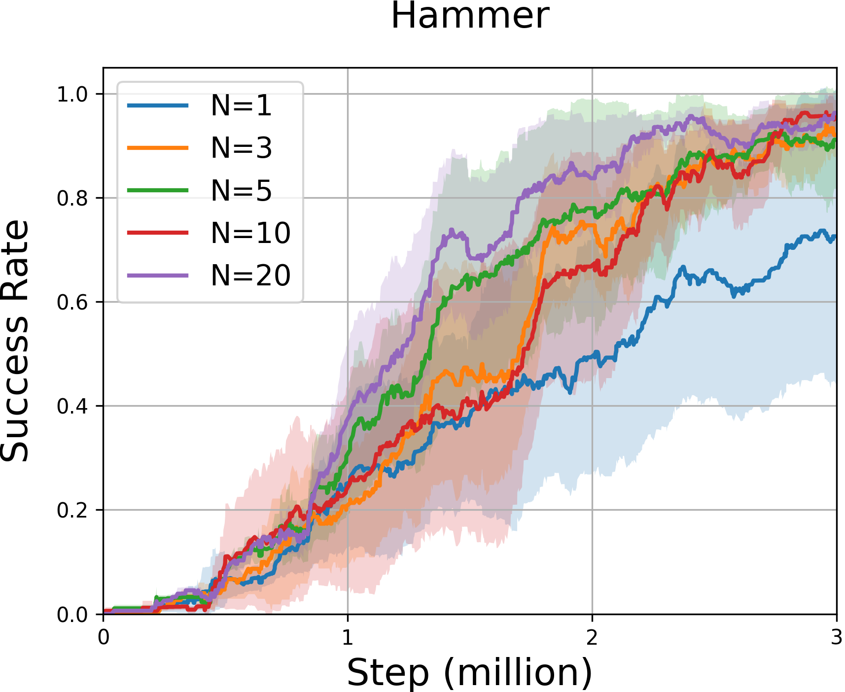
Adroit Experiments. We further delve into the Adroit continuous control tasks. In these challenges, a robot must skillfully manipulate a hand to perform various actions, such as adjusting a pen’s orientation or unlocking a door. Considering the complexity of the tasks and the robot’s high-dimensional state space, it becomes imperative to explore methods that can facilitate the robot’s learning. Figure 6 illustrates that our DRND method outperforms all the other methods in exploration, especially in the challenging ‘Hammer’ and ‘Relocate’ environments. However, in the ‘Pen’ environment, our method does not exhibit a significant improvement compared to other exploration algorithms. This could be attributed to the relatively simpler nature of this environment, which does not demand deep exploration.
Fetch Manipulation Tasks. The Fetch manipulation tasks involve various gym-robotics environments, challenging the Fetch robot arm with complex tasks like reaching, pushing, sliding, and pick-and-place actions. Due to their complexity, these tasks demand advanced exploration strategies. Our evaluation of exploration algorithms in this context highlights their effectiveness in handling intricate robotic manipulations. As shown in Figure 7, our DRND approach excels in assisting the robot in these tasks. Our DRND method effectively combines the strengths of these approaches, outperforming results achievable with either pseudo-count or curiosity-driven methods alone. Consequently, our DRND algorithm performs significantly better than the RND method and other exploration algorithms.
| Dataset | SAC | TD3+BC | CQL | IQL | SAC-RND | ReBRAC | SAC-DRND |
| hopper-random | 9.9 ± 1.5 | 8.5 ± 0.6 | 5.3 ± 0.6 | 10.1 ± 5.9 | 19.6 ± 12.4 | 8.1 ± 2.4 | 32.7 ± 0.4 |
| hopper-medium | 0.8 ± 0.0 | 59.3 ± 4.2 | 61.9 ± 6.4 | 65.2 ± 4.2 | 91.1 ± 10.1 | 102.0 ± 1.0 | 98.5 ± 1.1 |
| hopper-expert | 0.7 ± 0.0 | 107.8 ± 7.0 | 106.5 ± 9.1 | 108.8 ± 3.1 | 109.7 ± 0.5 | 100.1 ± 8.3 | 109.7 ± 0.3 |
| hopper-medium-expert | 0.7 ± 0.0 | 98.0 ± 9.4 | 96.9 ± 15.1 | 85.5 ± 29.7 | 109.8 ± 0.6 | 107.0 ± 6.4 | 108.7 ± 0.5 |
| hopper-medium-replay | 7.4 ± 0.5 | 60.9 ± 18.8 | 86.3 ± 7.3 | 89.6 ± 13.2 | 97.2 ± 9.0 | 98.1 ± 5.3 | 100.5 ± 1.0 |
| hopper-full-replay | 41.1 ± 17.9 | 97.9 ± 17.5 | 101.9 ± 0.6 | 104.4 ± 10.8 | 107.4 ± 0.8 | 107.1 ± 0.4 | 108.2 ± 0.7 |
| halfcheetah-random | 29.7 ± 1.4 | 11.0 ± 1.1 | 31.1 ± 3.5 | 19.5 ± 0.8 | 27.6 ± 2.1 | 29.5 ± 1.5 | 30.4 ± 4.0 |
| halfcheetah-medium | 55.2 ± 27.8 | 48.3 ± 0.3 | 46.9 ± 0.4 | 50.0 ± 0.2 | 66.4 ± 1.4 | 65.6 ± 1.0 | 68.3 ± 0.2 |
| halfcheetah-expert | -0.8 ± 1.8 | 96.7 ± 1.1 | 97.3 ± 1.1 | 95.5 ± 2.1 | 102.6 ± 4.2 | 105.9 ± 1.7 | 106.2 ± 3.7 |
| halfcheetah-medium-expert | 28.4 ± 19.4 | 90.7 ± 4.3 | 95.0 ± 1.4 | 92.7 ± 2.8 | 107.6 ± 2.8 | 101.1 ± 5.2 | 108.5 ± 1.1 |
| halfcheetah-medium-replay | 0.8 ± 1.0 | 44.6 ± 0.5 | 45.3 ± 0.3 | 42.1 ± 3.6 | 51.2 ± 3.2 | 51.0 ± 0.8 | 52.1 ± 4.8 |
| halfcheetah-full-replay | 86.8 ± 1.0 | 75.0 ± 2.5 | 76.9 ± 0.9 | 75.0 ± 0.7 | 81.2 ± 1.3 | 82.1 ± 1.1 | 81.4 ± 1.7 |
| walker2d-random | 0.9 ± 0.8 | 1.6 ± 1.7 | 5.1 ± 1.7 | 11.3 ± 7.0 | 18.7 ± 6.9 | 18.1 ± 4.5 | 21.7 ± 0.1 |
| walker2d-medium | -0.3 ± 0.2 | 83.7 ± 2.1 | 79.5 ± 3.2 | 80.7 ± 3.4 | 91.6 ± 2.8 | 82.5 ± 3.6 | 95.2 ± 0.7 |
| walker2d-expert | 0.7 ± 0.3 | 110.2 ± 0.3 | 109.3 ± 0.1 | 96.9 ± 32.3 | 104.5 ± 22.8 | 112.3 ± 0.2 | 114.0± 0.5 |
| walker2d-medium-expert | 1.9 ± 3.9 | 110.1 ± 0.5 | 109.1 ± 0.2 | 112.1 ± 0.5 | 104.6 ± 11.2 | 111.6 ± 0.3 | 109.6 ± 1.0 |
| walker2d-medium-replay | -0.4 ± 0.3 | 81.8 ± 5.5 | 76.8 ± 10.0 | 75.4 ± 9.3 | 88.7 ± 7.7 | 77.3 ± 7.9 | 91.0 ± 2.9 |
| walker2d-full-replay | 27.9 ± 47.3 | 90.3 ± 5.4 | 94.2 ± 1.9 | 97.5 ± 1.4 | 105.3 ± 3.2 | 102.2 ± 1.7 | 109.6 ± 0.7 |
| average score | 16.2 | 67.5 | 73.6 | 72.9 | 82.6 | 81.2 | 86.0 |
| Dataset | SAC | TD3+BC | CQL | IQL | SAC-RND | ReBRAC | SAC-DRND |
| antmaze-umaze | 0.0 | 78.6 | 74.0 | 83.3 ± 4.5 | 97.0 ± 1.5 | 97.8 ± 1.0 | 95.8 ± 2.4 |
| antmaze-umaze-diverse | 0.0 | 71.4 | 84.0 | 70.6 ± 3.7 | 66.0 ± 25.0 | 88.3 ± 13.0 | 87.2 ± 3.2 |
| antmaze-medium-play | 0.0 | 10.6 | 61.2 | 64.6 ± 4.9 | 38.5 ± 29.4 | 84.0 ± 4.2 | 86.2 ± 5.4 |
| antmaze-medium-diverse | 0.0 | 3.0 | 53.7 | 61.7 ± 6.1 | 74.7 ± 10.7 | 76.3 ± 13.5 | 83.0 ±3.8 |
| antmaze-large-play | 0.0 | 0.2 | 15.8 | 42.5 ± 6.5 | 43.9 ± 29.2 | 60.4 ± 26.1 | 53.2 ± 4.1 |
| antmaze-large-diverse | 0.0 | 0.0 | 14.9 | 27.6 ± 7.8 | 45.7 ± 28.5 | 54.4 ± 25.1 | 50.8 ± 10.5 |
| average score | 0.0 | 27.3 | 50.6 | 58.3 | 60.9 | 76.8 | 76.0 |
5.3 D4RL Offline experiments
We assessed our method using the D4RL (Fu et al., 2020) offline datasets, integrating the DRND approach with the SAC algorithm (Haarnoja et al., 2018). Considering all available datasets in each domain, we tested SAC-DRND on Gym-MuJoCo and the more intricate AntMaze D4RL tasks. Our analysis compares against notable algorithms as detailed in (Rezaeifar et al., 2022), including IQL (Kostrikov et al., 2021), CQL (Kumar et al., 2020), and TD3+BC (Fujimoto & Gu, 2021). It is worth noting that although our method also has target networks, they are fixed and not trained, making it ensemble-free. Our SAC-DRND is ensemble-free and only involves training double critics networks. We compare our methods against recent strong model-free offline RL algorithms in Table 3. Additionally, we compare SAC-DRND against strong ensemble-based algorithms like SAC-N in Appendix E.1. Only the results of the ensemble-free methods are shown in the main text. The results are evaluated at the final gradient step over 10 different seeds.
It can be seen that SAC-DRND excels in the majority of MuJoCo tasks, attaining the best results among all ensemble-free methods. On Antmaze tasks, DRND also reached a level similar to SOTA. Compared to SAC-RND, which has comparable computational and storage requirements as our approach, SAC-DRND more effectively captures the dataset distribution, as reflected in its superior average scores and decreased variance. We also conducted experiments on Adroit tasks (Appendix E.2), hyperparameters sensitivity experiments (Appendix E.3) using Expected Online Performance (EOP, (Kurenkov & Kolesnikov, 2022)) and offline-to-online experiments (Appendix E.8).
6 Conclusion
Our research highlights the “bonus inconsistency” issue inherent in RND, which hinders its capacity for deep exploration. We introduce DRND, which distills a random target from a random distribution. Our approach efficiently records state-action occurrences without substantial time and space overhead by utilizing specially designed statistics to extract pseudo-counts. Theoretical analysis and empirical results show our method’s effectiveness in tackling bonus inconsistency. We observe promising results across Atari games, gym-robotics tasks, and offline D4RL datasets.
Acknowledgements
This work was supported by the STI 2030-Major Projects under Grant 2021ZD0201404.
Impact Statement
This paper presents work whose goal is to advance the field of Machine Learning. There are many potential societal consequences of our work, none which we feel must be specifically highlighted here.
References
- Achiam & Sastry (2017) Achiam, J. and Sastry, S. Surprise-based intrinsic motivation for deep reinforcement learning. arXiv preprint arXiv:1703.01732, 2017.
- An et al. (2021) An, G., Moon, S., Kim, J.-H., and Song, H. O. Uncertainty-based offline reinforcement learning with diversified q-ensemble. Advances in neural information processing systems, 34:7436–7447, 2021.
- Azar et al. (2017) Azar, M. G., Osband, I., and Munos, R. Minimax regret bounds for reinforcement learning. In International Conference on Machine Learning, pp. 263–272. PMLR, 2017.
- Bellemare et al. (2016) Bellemare, M., Srinivasan, S., Ostrovski, G., Schaul, T., Saxton, D., and Munos, R. Unifying count-based exploration and intrinsic motivation. Advances in neural information processing systems, 29, 2016.
- Bradbury et al. (2018) Bradbury, J., Frostig, R., Hawkins, P., Johnson, M. J., Leary, C., Maclaurin, D., Necula, G., Paszke, A., VanderPlas, J., Wanderman-Milne, S., et al. Jax: composable transformations of python+ numpy programs. 2018.
- Burda et al. (2018a) Burda, Y., Edwards, H., Pathak, D., Storkey, A., Darrell, T., and Efros, A. A. Large-scale study of curiosity-driven learning. arXiv preprint arXiv:1808.04355, 2018a.
- Burda et al. (2018b) Burda, Y., Edwards, H., Storkey, A., and Klimov, O. Exploration by random network distillation. arXiv preprint arXiv:1810.12894, 2018b.
- Ciosek et al. (2019) Ciosek, K., Fortuin, V., Tomioka, R., Hofmann, K., and Turner, R. Conservative uncertainty estimation by fitting prior networks. In International Conference on Learning Representations, 2019.
- Fu et al. (2020) Fu, J., Kumar, A., Nachum, O., Tucker, G., and Levine, S. D4rl: Datasets for deep data-driven reinforcement learning. arXiv preprint arXiv:2004.07219, 2020.
- Fujimoto & Gu (2021) Fujimoto, S. and Gu, S. S. A minimalist approach to offline reinforcement learning. Advances in neural information processing systems, 34:20132–20145, 2021.
- Fujimoto et al. (2019) Fujimoto, S., Meger, D., and Precup, D. Off-policy deep reinforcement learning without exploration. In International conference on machine learning, pp. 2052–2062. PMLR, 2019.
- Ghasemipour et al. (2022) Ghasemipour, K., Gu, S. S., and Nachum, O. Why so pessimistic? estimating uncertainties for offline rl through ensembles, and why their independence matters. Advances in Neural Information Processing Systems, 35:18267–18281, 2022.
- Haarnoja et al. (2018) Haarnoja, T., Zhou, A., Abbeel, P., and Levine, S. Soft actor-critic: Off-policy maximum entropy deep reinforcement learning with a stochastic actor. In International conference on machine learning, pp. 1861–1870. PMLR, 2018.
- Hong et al. (2022) Hong, J., Kumar, A., and Levine, S. Confidence-conditioned value functions for offline reinforcement learning. arXiv preprint arXiv:2212.04607, 2022.
- Houthooft et al. (2016) Houthooft, R., Chen, X., Duan, Y., Schulman, J., De Turck, F., and Abbeel, P. Vime: Variational information maximizing exploration. Advances in neural information processing systems, 29, 2016.
- Jayakumar et al. (2020) Jayakumar, S. M., Czarnecki, W. M., Menick, J., Schwarz, J., Rae, J., Osindero, S., Teh, Y. W., Harley, T., and Pascanu, R. Multiplicative interactions and where to find them. 2020.
- Kim & Oh (2023) Kim, B. and Oh, M.-h. Model-based offline reinforcement learning with count-based conservatism. 2023.
- Kostrikov et al. (2021) Kostrikov, I., Nair, A., and Levine, S. Offline reinforcement learning with implicit q-learning. arXiv preprint arXiv:2110.06169, 2021.
- Kumar et al. (2020) Kumar, A., Zhou, A., Tucker, G., and Levine, S. Conservative q-learning for offline reinforcement learning. Advances in Neural Information Processing Systems, 33:1179–1191, 2020.
- Kurenkov & Kolesnikov (2022) Kurenkov, V. and Kolesnikov, S. Showing your offline reinforcement learning work: Online evaluation budget matters. In International Conference on Machine Learning, pp. 11729–11752. PMLR, 2022.
- Kuznetsov et al. (2020) Kuznetsov, A., Shvechikov, P., Grishin, A., and Vetrov, D. Controlling overestimation bias with truncated mixture of continuous distributional quantile critics. In International Conference on Machine Learning, pp. 5556–5566. PMLR, 2020.
- Lobel et al. (2022) Lobel, S., Gottesman, O., Allen, C., Bagaria, A., and Konidaris, G. Optimistic initialization for exploration in continuous control. In Proceedings of the AAAI Conference on Artificial Intelligence, volume 36, pp. 7612–7619, 2022.
- Lobel et al. (2023) Lobel, S., Bagaria, A., and Konidaris, G. Flipping coins to estimate pseudocounts for exploration in reinforcement learning. arXiv preprint arXiv:2306.03186, 2023.
- Lyu et al. (2022a) Lyu, J., Li, X., and Lu, Z. Double check your state before trusting it: Confidence-aware bidirectional offline model-based imagination. In Thirty-sixth Conference on Neural Information Processing Systems, 2022a.
- Lyu et al. (2022b) Lyu, J., Ma, X., Li, X., and Lu, Z. Mildly conservative q-learning for offline reinforcement learning. In Thirty-sixth Conference on Neural Information Processing Systems, 2022b.
- Lyu et al. (2023) Lyu, J., Gong, A., Wan, L., Lu, Z., and Li, X. State advantage weighting for offline RL. In International Conference on Learning Representation tiny paper, 2023. URL https://openreview.net/forum?id=PjypHLTo29v.
- Machado et al. (2020) Machado, M. C., Bellemare, M. G., and Bowling, M. Count-based exploration with the successor representation. In Proceedings of the AAAI Conference on Artificial Intelligence, volume 34, pp. 5125–5133, 2020.
- Martin et al. (2017) Martin, J., Sasikumar, S. N., Everitt, T., and Hutter, M. Count-based exploration in feature space for reinforcement learning. arXiv preprint arXiv:1706.08090, 2017.
- Nikulin et al. (2023) Nikulin, A., Kurenkov, V., Tarasov, D., and Kolesnikov, S. Anti-exploration by random network distillation. arXiv preprint arXiv:2301.13616, 2023.
- Osband et al. (2016) Osband, I., Blundell, C., Pritzel, A., and Van Roy, B. Deep exploration via bootstrapped dqn. Advances in neural information processing systems, 29, 2016.
- Ostrovski et al. (2017) Ostrovski, G., Bellemare, M. G., Oord, A., and Munos, R. Count-based exploration with neural density models. In International conference on machine learning, pp. 2721–2730. PMLR, 2017.
- Paszke et al. (2019) Paszke, A., Gross, S., Massa, F., Lerer, A., Bradbury, J., Chanan, G., Killeen, T., Lin, Z., Gimelshein, N., Antiga, L., et al. Pytorch: An imperative style, high-performance deep learning library. Advances in neural information processing systems, 32, 2019.
- Pathak et al. (2017) Pathak, D., Agrawal, P., Efros, A. A., and Darrell, T. Curiosity-driven exploration by self-supervised prediction. In International conference on machine learning, pp. 2778–2787. PMLR, 2017.
- Plappert et al. (2018) Plappert, M., Andrychowicz, M., Ray, A., McGrew, B., Baker, B., Powell, G., Schneider, J., Tobin, J., Chociej, M., Welinder, P., et al. Multi-goal reinforcement learning: Challenging robotics environments and request for research. arXiv preprint arXiv:1802.09464, 2018.
- Rajeswaran et al. (2017) Rajeswaran, A., Kumar, V., Gupta, A., Vezzani, G., Schulman, J., Todorov, E., and Levine, S. Learning complex dexterous manipulation with deep reinforcement learning and demonstrations. arXiv preprint arXiv:1709.10087, 2017.
- Rezaeifar et al. (2022) Rezaeifar, S., Dadashi, R., Vieillard, N., Hussenot, L., Bachem, O., Pietquin, O., and Geist, M. Offline reinforcement learning as anti-exploration. In Proceedings of the AAAI Conference on Artificial Intelligence, volume 36, pp. 8106–8114, 2022.
- Schulman et al. (2017) Schulman, J., Wolski, F., Dhariwal, P., Radford, A., and Klimov, O. Proximal policy optimization algorithms. arXiv preprint arXiv:1707.06347, 2017.
- Stadie et al. (2015) Stadie, B. C., Levine, S., and Abbeel, P. Incentivizing exploration in reinforcement learning with deep predictive models. arXiv preprint arXiv:1507.00814, 2015.
- Still & Precup (2012) Still, S. and Precup, D. An information-theoretic approach to curiosity-driven reinforcement learning. Theory in Biosciences, 131:139–148, 2012.
- Strehl & Littman (2008) Strehl, A. L. and Littman, M. L. An analysis of model-based interval estimation for markov decision processes. Journal of Computer and System Sciences, 74(8):1309–1331, 2008.
- Sutton et al. (1998) Sutton, R. S., Barto, A. G., et al. Introduction to reinforcement learning, volume 135. MIT press Cambridge, 1998.
- Tang et al. (2017) Tang, H., Houthooft, R., Foote, D., Stooke, A., Xi Chen, O., Duan, Y., Schulman, J., DeTurck, F., and Abbeel, P. # exploration: A study of count-based exploration for deep reinforcement learning. Advances in neural information processing systems, 30, 2017.
- Tarasov et al. (2022) Tarasov, D., Nikulin, A., Akimov, D., Kurenkov, V., and Kolesnikov, S. Corl: Research-oriented deep offline reinforcement learning library. arXiv preprint arXiv:2210.07105, 2022.
- Tarasov et al. (2023) Tarasov, D., Kurenkov, V., Nikulin, A., and Kolesnikov, S. Revisiting the minimalist approach to offline reinforcement learning. arXiv preprint arXiv:2305.09836, 2023.
- Wang et al. (2018) Wang, Q., Xiong, J., Han, L., Liu, H., Zhang, T., et al. Exponentially weighted imitation learning for batched historical data. Advances in Neural Information Processing Systems, 31, 2018.
- Wang et al. (2020) Wang, Z., Novikov, A., Zolna, K., Merel, J. S., Springenberg, J. T., Reed, S. E., Shahriari, B., Siegel, N., Gulcehre, C., Heess, N., et al. Critic regularized regression. Advances in Neural Information Processing Systems, 33:7768–7778, 2020.
- Wu et al. (2019) Wu, Y., Tucker, G., and Nachum, O. Behavior regularized offline reinforcement learning. arXiv preprint arXiv:1911.11361, 2019.
- Xie et al. (2021) Xie, T., Cheng, C.-A., Jiang, N., Mineiro, P., and Agarwal, A. Bellman-consistent pessimism for offline reinforcement learning. Advances in neural information processing systems, 34:6683–6694, 2021.
- Yang et al. (2022) Yang, R., Bai, C., Ma, X., Wang, Z., Zhang, C., and Han, L. Rorl: Robust offline reinforcement learning via conservative smoothing. Advances in Neural Information Processing Systems, 35:23851–23866, 2022.
Appendix A Proof
In this section, we will provide all the proofs in the main text.
A.1 proof of lemma 4.1
Since and are i.i.d., . So we have:
A.2 proof pf lemma 4.3
For simplicity, we use some symbols to record the moments of the distribution of :
The calculation of moment is as follows:
The statistic is:
and its expectation is:
This indicates that the statistic is an unbiased estimator for the reciprocal of the frequency of . The variance of is:
where
so we have:
When tends to infinity, the variance of the statistic tends to zero, which reflects the stability or consistency of .
Appendix B DRND Pseudo-code
|
|
|
|
|
|
|
|
Appendix C Implementation Details and Experimental Settings
Our experiments were performed by using the following hardware and software:
-
•
GPUs: NVIDIA GeForce RTX 3090
-
•
Python 3.10.8
-
•
Numpy 1.23.4
-
•
Gymnasium 0.28.1
-
•
Gymnasium-robotics 1.2.2
-
•
Pytorch 1.13.0
-
•
MuJoCo-py 2.1.2.14
-
•
MuJoCo 2.3.1
-
•
D4RL 1.1
-
•
Jax 0.4.13
The architecture of predictor networks in Figure 1 and Figure 3 is 3 linear layers, the input dim is 2, hidden dim and output dim is 16, activate function is ReLU. Target networks’ architecture is 2 linear layers, the input dim is 2, hidden dim and output dim is 16, activate function is ReLU. We set the state as 2-dimensional, with the state space defined as the 2-dimensional space [0,1]x[0,1]. The given distribution is regarded as the dataset distribution of the current agent passing through states, and the dimensions can be arbitrary. Setting it as 2-dimensional is merely for visualization convenience.
In our experiments, for a fair comparison, all methods employed the same predictor and target networks. The fundamental parameters of the base algorithm such as learning rate and batch size were kept identical across all methods. For the hyperparameters of the utilized exploration algorithms, we utilized the author-recommended hyperparameters from respective papers (e.g., CFN). Since the CFN method was originally proposed for off-policy strategies, it utilized a trick of importance sampling for sampling from the replay buffer. However, in our PPO-based approach, there is no replay buffer, and we consider the use of the importance sampling trick unfair compared to other methods. Therefore, we only employed the core formula from the paper as the intrinsic reward, where represents the output dimension of the predictor network.
In our D4RL experiments, all experiments use the dataset of the ‘v2’ version. We use specific hyperparameters for each task due to varying anti-exploration penalties. Because most of the offline experiment time is spent on gradient calculation of data, we use the faster Jax framework (Bradbury et al., 2018) than the Pytorch framework (Paszke et al., 2019) for the experiments. In the online experiments, we still use the easier-to-read and more portable Pytorch framework instead of the faster computing Jax framework because most of the online experiment time is spent interacting with the environment rather than gradient computing.
We employ the ‘NoFrameskip-v4’ version in our Atari game experiments to execute the environments. These experiments encompass 128 parallel environments and adhere to the default configurations and network architecture as delineated in (Burda et al., 2018b). For Adroit and Fetch manipulation tasks, we employ the ‘v0’ version for Adroit tasks and the ‘v2’ version for Fetch tasks. In the ‘Relocate’ task, we truncate the episode when the ball leaves the table. These tasks pose a significant challenge for conventional methods to learn from, primarily due to the dataset consisting of limited human demonstrations in a sparse-reward, complex, high-dimensional robotic manipulation task (Lyu et al., 2022a). We do not include random state restarts, as they may undermine the necessity for exploration by the observations made by (Lobel et al., 2022). To set the goal locations for the non-default versions of the tasks, we follow the setting of (Lobel et al., 2023).
In the context of the D4RL framework, we make specific architectural choices. Instead of simply concatenating the state and action dimensions, we employ a bilinear structure in the first layer, as proposed by (Jayakumar et al., 2020). Additionally, we apply FiLM (Feature-wise Linear Modulation) architecture on the penultimate layer before the nonlinearity. This modification is effective for offline tasks, as indicated by (Nikulin et al., 2023).
Appendix D Hyperparameters
The hyperparameters are shown in Table 6 in online experiments. We employ distinct parameters and networks for Atari games and continuous control environments because Atari game observations are images, while observations for Adroit and Fetch tasks consist of states. The hyperparameters we use in the D4RL offline experiment are shown in Table 4. In D4RL offline datasets, we apply varying scales in each experiment due to the differing dataset qualities, as illustrated in Table 5.
| Name | Description | Value |
|---|---|---|
| learning rate of the actor network | 1e-3 (1e-4 on Antmaze) | |
| learning rate of the critic network | 1e-3 (1e-4 on Antmaze) | |
| learning rate of the DRND network | 1e-6 (1e-5 on Antmaze) | |
| optimizer | type of optimizer | Adam |
| target entropy | target entropy of the actor | -action_dim |
| soft update rate | 0.005 | |
| discount return | 0.99 (0.999 on Antmaze) | |
| batch size of the dataset | 1024 | |
| number of hidden layer dimensions | 256 | |
| number of DRND output dimensions | 32 | |
| number of hidden layers | 4 | |
| activation function | ReLU | |
| number of DRND training epochs | 100 | |
| maximum iteration number of SAC | 3000 | |
| gradient updates per iteration | 1000 | |
| number of DRND target networks | 10 | |
| the scale of two intrinsic reward items | 0.9 |
| Dataset Name | ||
|---|---|---|
| hopper-random | 1.0 | 1.0 |
| hopper-medium | 15.0 | 15.0 |
| hopper-expert | 10.0 | 10.0 |
| hopper-medium-expert | 10.0 | 10.0 |
| hopper-medium-replay | 5.0 | 10.0 |
| hopper-full-replay | 2.0 | 2.0 |
| halfcheetah-random | 0.05 | 0.05 |
| halfcheetah-medium | 1.0 | 0.1 |
| halfcheetah-expert | 5.0 | 5.0 |
| halfcheetah-medium-expert | 0.1 | 0.1 |
| halfcheetah-medium-replay | 0.1 | 0.1 |
| halfcheetah-full-replay | 1.0 | 1.0 |
| walker2d-random | 1.0 | 1.0 |
| walker2d-medium | 10.0 | 10.0 |
| walker2d-expert | 5.0 | 5.0 |
| walker2d-medium-expert | 15.0 | 20.0 |
| walker2d-medium-replay | 5.0 | 10.0 |
| walker2d-full-replay | 3.0 | 3.0 |
| antmaze-umaze | 5.0 | 0.001 |
| antmaze-umaze-diverse | 3.0 | 0.001 |
| antmaze-medium-play | 3.0 | 0.005 |
| antmaze-medium-diverse | 2.0 | 0.001 |
| antmaze-large-play | 1.0 | 0.01 |
| antmaze-large-diverse | 0.5 | 0.01 |
| Name | Description | Value |
|---|---|---|
| learning rate of the actor network | 3e-4 (1e-4 on Atari) | |
| learning rate of the critic network | 3e-4 (1e-4 on Atari) | |
| learning rate of the DRND network | 3e-4 (1e-4 on Atari) | |
| optimizer | type of optimizer | Adam |
| soft update rate | 0.005 | |
| discount return | 0.99 | |
| coefficient of GAE | 0.95 | |
| PPO clip coefficient | 0.1 | |
| number of environments | 128 | |
| number of hidden layer dimensions | 64 (512 on Atari) | |
| number of output dimensions | 64 (512 on Atari) | |
| activation function | ReLU | |
| number of training epochs | 4 | |
| number of DRND target networks | 10 | |
| coefficient of intrinsic reward | 1 | |
| the scale of two intrinsic reward items | 0.9 |
Appendix E Additional Experimental Results
E.1 Comparing to Ensemble-based Methods
As described in (Osband et al., 2016), the ensemble method estimates the Q-posterior, leading to varied predictions and imposing significant penalties in regions with limited data. We add the results of ensemble-based methods like SAC-N (An et al., 2021), EDAC (An et al., 2021), and RORL (Yang et al., 2022). Table 7 displays our results in these experiments. An underlined number represents the peak value for ensemble-free methods, while a bold number denotes each task’s top score. SAC-DRND outperforms most ensemble-based methods, such as SAC-N and RORL, in total scores on most MuJoCo tasks. For Antmaze tasks, our method leads among ensemble-free approaches and holds its own against ensemble-based methods.
| Ensemble-free | Ensemble-based | Ours | ||||||||
| Dataset | SAC | TD3+BC | CQL | IQL | SAC-RND | ReBRAC | SAC-N | EDAC | RORL | SAC-DRND |
| hopper-random | 9.9 ± 1.5 | 8.5 ± 0.6 | 5.3 ± 0.6 | 10.1 ± 5.9 | 19.6 ± 12.4 | 8.1 ± 2.4 | 28.0 ± 0.9 | 25.3 ± 10.4 | 31.4 ± 0.1 | 32.7 ± 0.4 |
| hopper-medium | 0.8 ± 0.0 | 59.3 ± 4.2 | 61.9 ± 6.4 | 65.2 ± 4.2 | 91.1 ± 10.1 | 102.0 ± 1.0 | 100.3 ± 0.3 | 101.6 ± 0.6 | 104.8 ± 0.1 | 98.5 ± 1.1 |
| hopper-expert | 0.7 ± 0.0 | 107.8 ± 7.0 | 106.5 ± 9.1 | 108.8 ± 3.1 | 109.7 ± 0.5 | 100.1 ± 8.3 | 110.3 ± 0.3 | 110.1 ± 0.1 | 112.8 ± 0.2 | 109.7 ± 0.3 |
| hopper-medium-expert | 0.7 ± 0.0 | 98.0 ± 9.4 | 96.9 ± 15.1 | 85.5 ± 29.7 | 109.8 ± 0.6 | 107.0 ± 6.4 | 110.1 ± 0.3 | 110.7 ± 0.1 | 112.7 ± 0.2 | 108.7 ± 0.5 |
| hopper-medium-replay | 7.4 ± 0.5 | 60.9 ± 18.8 | 86.3 ± 7.3 | 89.6 ± 13.2 | 97.2 ± 9.0 | 98.1 ± 5.3 | 101.8 ± 0.5 | 101.0 ± 0.5 | 102.8 ± 0.5 | 100.5 ± 1.0 |
| hopper-full-replay | 41.1 ± 17.9 | 97.9 ± 17.5 | 101.9 ± 0.6 | 104.4 ± 10.8 | 107.4 ± 0.8 | 107.1 ± 0.4 | 102.9 ± 0.3 | 105.4 ± 0.7 | - | 108.2 ± 0.7 |
| halfcheetah-random | 29.7 ± 1.4 | 11.0 ± 1.1 | 31.1 ± 3.5 | 19.5 ± 0.8 | 27.6 ± 2.1 | 29.5 ± 1.5 | 28.0 ± 0.9 | 28.4 ± 1.0 | 28.5 ± 0.8 | 30.4 ± 4.0 |
| halfcheetah-medium | 55.2 ± 27.8 | 48.3 ± 0.3 | 46.9 ± 0.4 | 50.0 ± 0.2 | 66.4 ± 1.4 | 65.6 ± 1.0 | 67.5 ± 1.2 | 65.9 ± 0.6 | 66.8 ± 0.7 | 68.3 ± 0.2 |
| halfcheetah-expert | -0.8 ± 1.8 | 96.7 ± 1.1 | 97.3 ± 1.1 | 95.5 ± 2.1 | 102.6 ± 4.2 | 105.9 ± 1.7 | 105.2 ± 2.6 | 106.8 ± 3.4 | 105.2 ± 0.7 | 106.2 ± 3.7 |
| halfcheetah-medium-expert | 28.4 ± 19.4 | 90.7 ± 4.3 | 95.0 ± 1.4 | 92.7 ± 2.8 | 107.6 ± 2.8 | 101.1 ± 5.2 | 107.1 ± 2.0 | 106.3 ± 1.9 | 107.8 ± 1.1 | 108.5 ± 1.1 |
| halfcheetah-medium-replay | 0.8 ± 1.0 | 44.6 ± 0.5 | 45.3 ± 0.3 | 42.1 ± 3.6 | 51.2 ± 3.2 | 51.0 ± 0.8 | 63.9 ± 0.8 | 61.3 ± 1.9 | 61.9 ± 1.5 | 52.1 ± 4.8 |
| halfcheetah-full-replay | 86.8 ± 1.0 | 75.0 ± 2.5 | 76.9 ± 0.9 | 75.0 ± 0.7 | 81.2 ± 1.3 | 82.1 ± 1.1 | 84.5 ± 1.2 | 84.6 ± 0.9 | - | 81.4 ± 1.7 |
| walker2d-random | 0.9 ± 0.8 | 1.6 ± 1.7 | 5.1 ± 1.7 | 11.3 ± 7.0 | 18.7 ± 6.9 | 18.1 ± 4.5 | 21.7 ± 0.0 | 16.6 ± 7.0 | 21.4 ± 0.2 | 21.7 ± 0.1 |
| walker2d-medium | -0.3 ± 0.2 | 83.7 ± 2.1 | 79.5 ± 3.2 | 80.7 ± 3.4 | 91.6 ± 2.8 | 82.5 ± 3.6 | 87.9 ± 0.2 | 92.5 ± 0.8 | 102.4 ± 1.4 | 95.2 ± 0.7 |
| walker2d-expert | 0.7 ± 0.3 | 110.2 ± 0.3 | 109.3 ± 0.1 | 96.9 ± 32.3 | 104.5 ± 22.8 | 112.3 ± 0.2 | 107.4 ± 2.4 | 115.1 ± 1.9 | 115.4 ± 0.5 | 114.0± 0.5 |
| walker2d-medium-expert | 1.9 ± 3.9 | 110.1 ± 0.5 | 109.1 ± 0.2 | 112.1 ± 0.5 | 104.6 ± 11.2 | 111.6 ± 0.3 | 116.7 ± 0.4 | 114.7 ± 0.9 | 121.2 ± 1.5 | 109.6 ± 1.0 |
| walker2d-medium-replay | -0.4 ± 0.3 | 81.8 ± 5.5 | 76.8 ± 10.0 | 75.4 ± 9.3 | 88.7 ± 7.7 | 77.3 ± 7.9 | 78.7 ± 0.7 | 87.1 ± 2.4 | 90.4 ± 0.5 | 91.0 ± 2.9 |
| walker2d-full-replay | 27.9 ± 47.3 | 90.3 ± 5.4 | 94.2 ± 1.9 | 97.5 ± 1.4 | 105.3 ± 3.2 | 102.2 ± 1.7 | 94.6 ± 0.5 | 99.8 ± 0.7 | - | 109.6 ± 0.7 |
| average score | 16.2 | 67.5 | 73.6 | 72.9 | 82.6 | 81.2 | 84.4 | 85.2 | 85.7 | 86.0 |
| Dataset | SAC | TD3+BC | CQL | IQL | SAC-RND | ReBRAC | RORL | MSG | SAC-DRND |
| antmaze-umaze | 0.0 | 78.6 | 74.0 | 83.3 ± 4.5 | 97.0 ± 1.5 | 97.8 ± 1.0 | 97.7 ± 1.9 | 97.9 ± 1.3 | 95.8 ± 2.4 |
| antmaze-umaze-diverse | 0.0 | 71.4 | 84.0 | 70.6 ± 3.7 | 66.0 ± 25.0 | 88.3 ± 13.0 | 90.7 ± 2.9 | 79.3 ± 3.0 | 87.2 ± 3.2 |
| antmaze-medium-play | 0.0 | 10.6 | 61.2 | 64.6 ± 4.9 | 38.5 ± 29.4 | 84.0 ± 4.2 | 76.3 ± 2.5 | 85.9 ± 3.9 | 86.2 ± 5.4 |
| antmaze-medium-diverse | 0.0 | 3.0 | 53.7 | 61.7 ± 6.1 | 74.7 ± 10.7 | 76.3 ± 13.5 | 69.3 ± 3.3 | 84.6 ± 5.2 | 83.0 ±3.8 |
| antmaze-large-play | 0.0 | 0.2 | 15.8 | 42.5 ± 6.5 | 43.9 ± 29.2 | 60.4 ± 26.1 | 16.3 ± 11.1 | 64.3 ± 12.7 | 53.2 ± 4.1 |
| antmaze-large-diverse | 0.0 | 0.0 | 14.9 | 27.6 ± 7.8 | 45.7 ± 28.5 | 54.4 ± 25.1 | 41.0 ± 10.7 | 71.3 ± 5.3 | 50.8 ± 10.5 |
| average score | 0.0 | 27.3 | 50.6 | 58.3 | 60.9 | 76.8 | 65.2 | 80.5 | 76.0 |
E.2 Results on Adroit Tasks
In this subsection, we show the scores of SAC-DRND on Adroit tasks in Table 8.
| Task Name | BC | TD3+BC | IQL | CQL | SAC-RND | ReBRAC | SAC-DRND |
|---|---|---|---|---|---|---|---|
| pen-human | 34.4 | 81.8 ± 14.9 | 81.5 ± 17.5 | 37.5 | 5.6 ± 5.8 | 103.5 ± 14.1 | 42.3 ± 11.8 |
| pen-cloned | 56.9 | 61.4 ± 19.3 | 77.2 ± 17.7 | 39.2 | 2.5 ± 6.1 | 91.8 ± 21.7 | 39.5 ± 33.4 |
| pen-expert | 85.1 | 146.0 ± 7.3 | 133.6 ± 16.0 | 107.0 | 45.4 ± 22.9 | 154.1 ± 5.4 | 65.0 ± 17.1 |
| door-human | 0.5 | -0.1 ± 0.0 | 3.1 ± 2.0 | 9.9 | 0.0 ± 0.1 | 0.0 ± 0.0 | 1.3 ± 0.8 |
| door-cloned | -0.1 | 0.1 ± 0.6 | 0.8 ± 1.0 | 0.4 | 0.2 ± 0.8 | 1.1 ± 2.6 | 0.3 ± 0.1 |
| door-expert | 34.9 | 84.6 ± 44.5 | 105.3 ± 2.8 | 101.5 | 73.6 ± 26.7 | 104.6 ± 2.4 | 85.3 ± 37.9 |
| hammer-human | 1.5 | 0.4 ± 0.4 | 2.5 ± 1.9 | 4.4 | -0.1 ± 0.1 | 0.2 ± 0.2 | 0.3 ± 0.2 |
| hammer-cloned | 0.8 | 0.8 ± 0.7 | 1.1 ± 0.5 | 2.1 | 0.1 ± 0.4 | 6.7 ± 3.7 | 1.1 ± 0.8 |
| hammer-expert | 125.6 | 117.0 ± 30.9 | 129.6 ± 0.5 | 86.7 | 24.8 ± 39.4 | 133.8 ± 0.7 | 37.1 ± 47.2 |
| relocate-human | 0.0 | -0.2 ± 0.0 | 0.1 ± 0.1 | 0.2 | 0.0 ± 0.0 | 0.0 ± 0.0 | 0.0 ± 0.1 |
| relocate-cloned | -0.1 | -0.1 ± 0.1 | 0.2 ± 0.4 | -0.1 | 0.0 ± 0.0 | 0.9 ± 1.6 | 0.0 ± 0.0 |
| relocate-expert | 101.3 | 107.3 ± 1.6 | 106.5 ± 2.5 | 95.0 | 3.4 ± 4.5 | 106.6 ± 3.2 | 10.1 ± 7.1 |
| Average w/o expert | 11.7 | 18.0 | 20.8 | 11.7 | 1.0 | 25.5 | 10.6 |
| Average | 36.7 | 49.9 | 53.4 | 40.3 | 12.9 | 58.6 | 23.5 |
E.3 Expected Online Performance
We calculated the EOP on Gym-MuJoCo and AntMaze tasks, as shown in Table 9.
| Domain | Algorithm | 1 policy | 2 policies | 3 policies | 5 policies | 10 policies | 15 policies | 20 policies |
|---|---|---|---|---|---|---|---|---|
| Gym-MuJoCo | TD3+BC | 49.8 ± 21.4 | 61.0 ± 14.5 | 65.3 ± 9.3 | 67.8 ± 3.9 | - | - | - |
| IQL | 65.0 ± 9.1 | 69.9 ± 5.6 | 71.7 ± 3.5 | 72.9 ± 1.7 | 73.6 ± 0.8 | 73.8 ± 0.7 | 74.0 ± 0.6 | |
| ReBRAC | 62.0 ± 17.1 | 70.6 ± 9.9 | 73.3 ± 5.5 | 74.8 ± 2.1 | 75.6 ± 0.8 | 75.8 ± 0.6 | 76.0 ± 0.5 | |
| SAC-DRND | 69.9 ± 30.1 | 73.2 ± 19.0 | 79.4 ± 11.9 | 82.5 ± 7.8 | 84.0 ± 6.0 | 84.9 ± 3.1 | 85.3 ± 2.0 | |
| AntMaze | TD3+BC | 6.9 ± 7.0 | 10.7 ± 6.8 | 13.0 ± 6.0 | 15.5 ± 4.6 | - | - | - |
| IQL | 29.8 ± 15.5 | 38.0 ± 15.4 | 43.1 ± 13.8 | 48.7 ± 10.2 | 53.2 ± 4.4 | 54.3 ± 2.1 | 54.7 ± 1.2 | |
| ReBRAC | 67.9 ± 10.0 | 73.6 ± 7.4 | 76.1 ± 5.5 | 78.3 ± 3.4 | 79.9 ± 1.7 | 80.4 ± 1.1 | - | |
| SAC-DRND | 69.3 ± 15.9 | 75.3 ± 10.1 | 78.5 ± 7.6 | 81.5 ± 4.0 | 83.7 ± 3.1 | 84.5 ± 1.5 | 84.9 ± 0.9 |
We also show the EOP line for each task, as shown in Figure 8.


E.4 Parameter Study on the Number of Target Network
Our study explored the relationship between the number of different targets and their corresponding final scores in both online MuJoCo tasks and D4RL offline tasks. In our approach, if is not equal to 1, then must satisfy the condition . In the following charts, we fill in the values of RND at as a reference for the single target network results.
E.4.1 Online Tasks
We conduct adversarial attack experiments with different numbers of target networks in DRND. As shown in Figure 9, the robustness of DRND generally improves with an increase in the target number . Considering both runtime and performance, we chose as the optimal number of targets for our online experiments.


E.4.2 Offline Tasks
The results are shown in Table LABEL:target. The results indicate that the average score demonstrates an upward trend as the number of targets increases. At the same time, its variance decreases, which suggests that a higher number of targets generally leads to improved and more consistent outcomes. However, it’s worth noting that there are diminishing returns; for instance, the differences between the results at and are marginal. Considering these considerations, we chose for our offline experiments. Furthermore, the algorithm exhibits limited sensitivity to variations in the number of targets in online and offline settings.
| hopper-medium | 92.1 ± 8.4 | 93.3 ± 3.7 | 97.8 ± 2.4 | 98.5 ± 1.1 | 99.0 ± 0.6 |
| halfcheetah-medium | 66.4 ± 1.4 | 65.8 ± 1.8 | 66.7 ± 0.6 | 67.3 ± 0.2 | 67.4 ± 0.4 |
| walker2d-medium | 91.6 ± 2.8 | 94.5 ± 0.9 | 94.0 ± 1.6 | 95.2 ± 1.2 | 94.7 ± 1.2 |
| average score | 83.4 | 84.5 | 86.2 | 87.0 | 87.0 |
E.5 Runtime comparison
To verify no significant increase in computational overhead between our method and the RND method, we conducted experiments on the medium datasets in the offline D4RL tasks, comparing the computational costs of both methods, as shown in Figure 10. It can be observed that the runtime of our method is slightly less than that of the RND method. And it can be seen that as the number of targets increases, the running time does not significantly improve.

E.6 Parameter Study on
In this subsection, we provide the results of different with both online and offline tasks. We use varying .
E.6.1 Online Tasks
We study the performance under attacks with different in online tasks. We chose Adroit continuous control environments as our experiment environments. In the results shown in Figure 11, We observed that the performance is excellent when or in all four environments. The performance when is not as good as when , which indirectly confirms the effect of the second bonus term. We chose as the hyperparameter for our online experiments.


E.6.2 Offline Tasks
We examine the influence of on offline tasks using the D4RL dataset. We employ various values of to train an offline agent on the ‘medium’ datasets. The final scores are presented in Table LABEL:alpha, and the training curves are shown in Figure 12. It is observed that in some cases, when , the final score is higher, and the training curve exhibits greater stability. Consequently, we consistently opted for in our offline experiments. When , only the first bonus term comes into play, and the results are not as favorable as when , demonstrating the effectiveness of the second bonus term. Additionally, when examining the final results, it becomes evident that our first bonus outperforms the RND.
Also, for ease of comparison, we provide the training curves of SAC-RND on three datasets: hopper-medium, halfcheetah-medium, and walker2d-medium in Figure 14.


| SAC-RND | ||||||
|---|---|---|---|---|---|---|
| hopper-medium | 54.0 ± 31.1 | 42.3 ± 4.95 | 85.5 ± 8.7 | 98.5 ± 5.6 | 91.9 ± 4.9 | 91.1 ± 10.1 |
| halfcheetah-medium | 65.3 ± 1.3 | 67.5 ± 1.2 | 67.3 ± 0.6 | 68.6± 0.4 | 67.1 ± 0.2 | 66.4 ± 1.4 |
| walker2d-medium | -0.0 ± 0.1 | 3.1 ± 1.7 | 27.6 ± 31.9 | 94.7 ± 1.0 | 93.0 ± 1.8 | 91.6 ± 2.8 |
| average score | 39.8 | 37.6 | 60.1 | 87.2 | 84.0 | 83.0 |
E.7 Parameter Study on
We present the results of our parameter study on , which are detailed in the table below. We choose some environments and show the results. All experiments are conducted across 5 seeds, and we report the mean and standard deviation of their results.
| - | - | ||
| - | - |
| - | - | ||
| - | - |
| - | - | ||
| - | - |
| - | - | ||
| - | - |
| - | - | ||
| - | - |
| - | - | ||
| - | - |
E.8 Evaluation on offline-to-online D4RL
We report offline-to-online performance on AntMaze tasks. We followed the methodology outlined by (Tarasov et al., 2022). We report the scores after the offline stage and online tuning in Table 18.
| Task Name | TD3+BC | IQL | ReBRAC | SAC-DRND |
|---|---|---|---|---|
| antmaze-umaze | 66.8 91.4 | 77.00 96.50 | 97.8 99.8 | 95.8 98.3 |
| antmaze-umaze-diverse | 59.1 48.4 | 59.50 63.75 | 85.7 98.1 | 87.2 98.0 |
| antmaze-medium-play | 59.2 94.8 | 71.75 89.75 | 78.4 97.7 | 86.2 98.3 |
| antmaze-medium-diverse | 62.6 94.1 | 64.25 92.25 | 78.6 98.5 | 83.0 95.9 |
| antmaze-large-play | 21.5 0.1 | 38.5 64.50 | 47.0 39.5 | 53.2 51.5 |
| antmaze-large-diverse | 9.5 0.4 | 26.75 64.25 | 66.7 77.6 | 50.8 55.9 |
| Average | 46.4 54.8(+8.4) | 56.29 78.50(+22.21) | 75.7 85.2(+8.5) | 76.0 83.0(+7.0) |
E.9 More Detailed Change Process of RND Bonus


