Exploiting the Einstein Telescope to solve the Hubble tension
Abstract
We probe four cosmological models which, potentially, can solve the Hubble tension according to the dark energy equation of state. In this context, we demonstrate that the Einstein Telescope is capable of achieving a relative accuracy below on the Hubble constant independently of the specific dark energy model. We firstly build mock catalogs containing gravitational wave events for one, five and ten years of observations, and above Signal-to-Noise Ratio equal to nine. From these catalogs, we extract the events which are most likely associated with possible electromagnetic counterpart detected by THESEUS. Finally, we select four dark energy models, namely a non-flat CDM, an interacting dark energy, an emergent dark energy, and a time varying gravitational constant model, to forecast the precision down to which the Einstein Telescope can bound the corresponding cosmological parameters. We foresee that the Hubble constant is always constrained with less than uncertainty, thereby offering a potential solution to the Hubble tension. The accuracy on the other cosmological parameters is at most comparable with the one currently obtained using multiple probes, except for the emergent dark energy model for which the Einstein Telescope alone will be able to improve the current limits by more than one order of magnitude.
I Introduction
The detection of Gravitational Waves (GWs) from the coalescence of merging Binary Black Holes (BBH) and Binary Neutron Stars (BNS) [1, 2] opened a new window to test the General Relativity, relativistic astrophysics, and cosmology [2, 3, 4]. As it is well known, the GWs bring direct information on the luminosity distance of sources and, therefore, they can be used as rulers to measure distances in the Universe. Indeed, they are usually called standard sirens [5, 6], and are fully complementary to the standard candles, such as Cepheids and Supernovae Type Ia (SNeIa) among the others, that are instead based on the detection of their electromagnetic emission and need to be calibrated on closer sources in order to get a measure of their luminosity distance. Although GWs offer an alternative method to obtain distances in cosmology and are not affected by calibration problems, they are not free of issues. Indeed, the GWs waveform encodes both information on the systems, such as masses, spin, and inclination angle among others, and information on the cosmology such as the distance. Furthermore, they encode information on a given theory of gravity and, potentially, can probe it [7, 8, 9]. However, information on masses and redshift is completely degenerate, and the only way to break such degeneracy is to have prior information on the redshift from an electromagnetic counterpart. There are several ways to get accurate information on the redshift. For instance, one can assign to the GWs source the redshift of the host galaxy [5, 6, 10] or, alternatively, looking at the electromagnetic emission following the GWs such as short Gamma-Ray Burst (GRB) [11, 2] and kilonovae [2]. However, the host galaxy can be accurately detected only up to redshift below one [12], and kilonovae will be detected up to redshift [13]. On the contrary, short GRBs may be detected using forthcoming satellites, such as Transient High Energy Sources and Early Universe Surveyor (THESEUS), up to redshift [14, 15, 16]. Such high redshift detections can allow also to deeply test the cosmological evolution [17, 18, 19, 20]. Furthermore, a complementary avenue to obtain the redshift information is represented by the observation of tidal deformation in BNS mergers [21, 22]. Indeed, it may supply redshift estimation with an accuracy ranging from % to % depending on the choice of the equation of state (EoS).
Nowadays, the LIGO/Virgo/KAGRA collaborations have explored several ways to constrain cosmological models from GWs events. A turning point was the event GW170817, i.e. the first merger of a BNS with the simultaneous detection of the GRB 170817A [2], yielding to the first estimation of the Hubble constant with GWs, km s-1 Mpc-1 at 68% of confidence level [23]. Afterward, the LIGO/Virgo/KAGRA collaborations have explored the possibility to constrain by analyzing the population distribution of BBH mergers, and searching for the host galaxy identification [24]. However, these new measurements of the Hubble constant are in agreement with both the late-time and the early-time measurements of and, therefore, do not help to solve the so-called Hubble tension [25, 26, 27, 28, 29] which may, however, be alleviated to a 2.1 tension if the errors on the Hubble constant were underestimated [30]. Other examples of solutions to the Hubble tension may rely on modifications of fundamental laws [31, 32, 33]. Nevertheless, the next generation of GW detectors, e.g. the Einstein Telescope (ET), can strongly improve the accuracy on the Hubble constant reducing it below 1% [34, 35], and promise to offer a solution to such a tension pointing out its correct value. Therefore, there is an important need to study also the theoretical framework related to the Hubble tension. Let us remember that the Hubble tension is discrepancy between the measurements of obtained by fitting the CMB power spectra [36], and using the standard candles such as Cepheids [37] both in the framework of the concordance cosmological model, also known as Cold Dark Matter (CDM) model.
Since the nature of Dark Energy (DE) is still a puzzle (for a comprehensive review see Ref. [26]), there are many attempts to explain the tension modifying the DE EoS [38, 39, 25, 26, 40, 41], or the underlying theory of gravity [42, 43, 26, 44]. Several analyses have been carried out to measure the Hubble constant and DE EoS with GWs making use of different techniques such as the identification of the electromagnetic counterpart of GW sources [45, 46, 47], the cross-correlation between GW sources and galaxies [48], the statistical host identification techniques with galaxies [12, 49, 50, 51, 52], the hierarchical inference without galaxy surveys [53, 54, 55], the study of lensed events [56, 57] and the analysis of NS EoS [58, 59, 60].
It is worth noting that the CDM model has its own issues such as, for instance, the well-known small-scale problem of the CDM paradigm and the extremely small value of the cosmological constant compared to the expectation from quantum field theory [61]. Therefore, alternative approaches have been considered to overcome both the lack of experimental detection of the dark ingredients and the small-scale issues of CDM as well. For instance, the modification of the underlying theory of gravity can explain the acceleration of the Universe by means of extra degrees of freedom arising from higher-order curvature invariants or extra scalar fields [62, 63]. Alternatively, models of non-homogeneous universes or violations of the Copernican principle can also account for the accelerated expansion [64, 65]. Nevertheless, the debate on whether there is or not a real need to shift from the CDM to a more complicated model is still under debate [66].
Here, we will focus on a set of models which modify the DE EoS in view of solving the Hubble tension [25, 26]. For each model, we will predict the accuracy down to which ET will be able to detect departures from the CDM offering in such a way a theoretical framework of DE capable of solving the Hubble tension. In Sec. II, we will briefly introduce the DE models. In Sec. III, we will summarize the procedure adopted to build mock data that will mimic the ET observations of the luminosity distance. In Sec. IV, we will give details of our statistical analysis, while in Sec. V we will show results. Finally, in Sec. VI we will give our final discussion and conclusions.
II Dark Energy models
We focus on four DE models which may help in solving the Hubble tension [25, 26, 67, 68], and differ from each other in the way they affect the DE EoS leading to a modification of the luminosity distance. In the context of General Relativity, and of the Friedman–Lemaître–Robertson–Walker (FLRW) cosmology, the luminosity distance is defined as
| (1) |
where is the redshift, is the speed of light, is the Hubble constant, is the value of the curvature parameter at , and
| (2) |
where is the value of the matter density parameter at , and is the DE density parameter as a function of the redshift. In the CDM model, . Since Eq. (2) is strictly related to the Friedman equations and to the DE EoS, changing the DE model leads to different expressions of the function [69]. To study the proprieties of DE component in a general framework, one can consider the ratio of the DE pressure to its energy density as a function of redshift [70, 71]:
| (3) |
Again, CDM model is recovered for . In the next subsections, we will discuss four DE models whose modifications of the Eq. (2) may serve to solve the Hubble tension. Moreover, we will also discuss the limits in which such models recover the CDM cosmology.
II.1 Non-flat CDM
We focus on the simplest extension of the CDM model in which is a constant, but it can assume values different from , i.e. the cosmological constant. Hence, the modification to Eq. (2) appears as [72]
| (4) |
In [73], it was shown using the CMB + BAO + SN + dataset observations, the aforementioned model may solve the Hubble tension at 95% Confidence Level (CL). The best-fit values are: km s-1 Mpc-1 and . In [39], generating a mock dataset of combined events by ET and THESEUS, they obtained the following accuracy on the cosmological parameter :
II.2 Interacting Dark Energy
Another scenario capable of solving the Hubble tension considers that Dark Matter (DM) and DE interact not only gravitationally. This is the so-called Interacting Dark Energy (IDE) model. Following [75, 76], one can parameterize the interaction between DM and DE as follows
| (5) | ||||
| (6) |
where and are the energy-momentum tensors for the DM and DE, respectively. The coefficient encodes the coupling between the two dark components. Although different functional forms of have been explored [76, 77, 78], we select the following coupled model: ; because a generic interaction coupling might have several instabilities, while the model we choose can avoid them under some suitable conditions on and [76, 77]. Hence, the DM and DE background evolve with respect to the cosmic time as [76]
| (7) | ||||
| (8) |
Since the DM density must be positive along the cosmic evolution if and , we need to impose the following condition: [76].
Solving the Eqs. (7) and (8), one can rewrite the Eq. (2) for the case of an IDE model as
| (9) | |||
where . In order to avoid the early time instability, the quantities and must have opposite sign [76]. It is worth noticing that the CDM is recovered by setting and . In our analysis, we will consider two cases: (i) is fixed to and is a free parameter, (ii) and are both free parameters.
Using the CMB dataset, it has been shown, for case (i), that the IDE model is capable of solving the Hubble tension making early and late time measurements of agree at 68% CL [79, 80, 81]. The best-fit values are: km s-1 Mpc-1 and . In the case (ii), using CMB+Cepehids, the best-fit values are: km s-1 Mpc-1, and .
II.3 Emergent Dark Energy
Another solution to the Hubble constant is that DE contributes to the total energy density budget of the Universe only at late time [82, 83]. In such a case, the Eq. (2) can be re-written as follows
| (10) |
In the simplest parameterization, the DE evolves as [82]
| (11) |
In this parameterization, there are the same degrees of freedom of the CDM model. Indeed, there is only one free parameter, namely . Despite this is not a sever modification of the parameter space, the statistical analysis of the temperature fluctuations of the CMB data data [36] provides a higher value of the Hubble constant, [84], with respect to the CDM cosmology, which results to agree with the late-time measurements of at 68% CL.
We will focus on a generalization of the aforementioned model where the DE contribution arises at a specific transition redshift . In such a model the DE critical density can be written as [85]
| (12) |
where is a free parameter and is the epoch where the matter-energy density and the DE density are equal. More precisely, is defined by the following equality:
| (13) |
In this case, there is only one extra free parameter, , which can discriminate between the CDM model, which is recovered for , and the emergent DE parameterization given in Eqs. (10) and (12), with . Under the parameterization in Eq. (12), it has been shown using CMB+BAO+Cepheids that the tension reduces to with the best-fit values of and [86].
Finally, we focus on the second parameterization in Eq. (12) because it admits a direct limit to the CDM cosmological model and, therefore, allows us to predict the accuracy down to which departure from the CDM model may be detected by future experiments.
II.4 Time-Varying Gravitational Constant
Alternatively to the previous models, one can investigate the case in which gravitational coupling is a function of the redshift through some scalar field [87]. Starting from an effective quantum theory of gravity that is asymptotically safe, one can obtain [88, 89]. The term refers to the values of gravitational constant at , and parameterizes its evolution with redshift. Indeed, means that the gravitation constant is the Newtonian one, and no evolution with redshift is considered. Since the gravitational coupling is no longer a constant, the cosmological constant would also be redshift-dependent: [90]. The density of matter and of DE evolve according to the following equations:
| (14) | ||||
| (15) |
Therefore, the Eq. (2) can be recast in the following form
| (16) |
The requirement for a flat Universe leads to the relation [90]
| (17) |
Let us notice that the CDM cosmology is recovered by setting . Using the CMB + BAO + SN + dataset, it was shown that the model mitigates the tension in the Hubble constant reducing it at [73]. In their analysis, the best-fit values are: and .
II.5 Comparing the dark energy models with the CDM cosmology
In Fig. 1, we illustrate the impact of the DE parameters on the luminosity distance for each model. In the upper left panel, we depict the non-flat -CDM model for the value of as red and green solid lines, respectively. In the upper right panel, we show the IDE model for the value of as red and green solid lines, respectively. In the lower-left panel, we depict the emergent DE model for the value of as red and green solid lines, respectively. And, finally, in the lower right panel, we show the time-varying gravitational constant model for the value of as red and green solid lines, respectively. In all panels, we also report, for comparison, our fiducial cosmological model, as a blue solid line, which is a flat-CDM with the following values of cosmological parameters [36]:
| (18) | |||
Below each panel, we report the residuals to illustrate the level of departure expected from the CDM model. The maximum departure in the case of non-flat -CDM model is , while it reaches at for the IDE model. The emergent DE model reaches a maximum departure when as the model claims to solve the Hubble tension with a modification of the DE contribution at a late-time. Finally, the departure of the time-varying gravitational constant model from the fiducial model reaches at .

III Mock Data
Here we briefly summarize the procedure adopted to build up the mock catalogs. We closely follow the recipe given in [91], and assign the redshift to the GWs sources extracting it from the following redshift probability distribution [92, 93, 39]
| (19) |
where is a normalization factor, is the comoving volume element, and is the merger rate per unit of volume in the source frame. The latter takes the form [94, 95, 96]
| (20) |
where is the Star Formation Rate (SFR), and is the time delay distribution. We assume, for the SFR, the model proposed in [97] and for the time delay distribution a power law functional form, , as suggested by population synthesis models [98, 99, 100, 101, 102]. Nevertheless, it is worth noticing that setting the SFR and the time delay distribution to other models do not affect the accuracy of final results (for more details we refer to Sec. 5.3 in [91]). We integrate Eq. (20) between a minimum time delay of Myr and the maximum fixed to the Hubble time. Furthermore, the quantity is the normalization of the merger rate at . We, therefore, set it to the best-fit value obtained by the LIGO/Virgo/KAGRA collaboration: [103]. Once the redshift is extracted from the probability distribution in Eq. (19), we can assign a fiducial luminosity distance, , based on our fiducial cosmological model in Eq. (18).
The ET will have three independent interferometers and, hence, the combined SNR is . The SNR of the single interferometer, , in the ideal case of Gaussian noise, is:
| (21) |
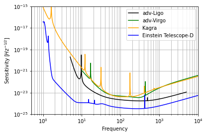
In the previous definition, is the one-sided noise power spectral density of -th interferometer, and are the GW strain amplitudes of and polarizations, and and are the so-called beam pattern functions [104]. The whole sensitivity function111The latest power spectral density can be downloaded at https://apps.et-gw.eu/tds/?content=3&r=14065. is depicted in in Fig. 2 . To integrate Eq. (21), we set a lower cutoff, , at Hz [105] and the upper one to .
We can compute the total number of observable BNS mergers, , from the equation
| (22) |
where is the duty cycle and is the observation time. In order to generate the catalog and select the events above a certain threshold of the signal-to-noise ratio (SNR) , we assume an isotropic distribution for the sky angles and , and an uniform distribution for the orientation angle and the polarization . Moreover, to generate the synthetic signal self-consistently with our choice of , we follow the LIGO/Virgo/KAGRA collaboration and set a uniform NS mass range in the interval . Thus, we obtain a rate of events per year, assuming a duty cycle of 80%. In our analysis, we will consider 1, 5, and 10 years of observations.
Once the fiducial luminosity distances are generated, we add a Gaussian noise component, , to them in order generate our mock observations. The variance includes the contributions due to the instrument, , the lensing, , and the peculiar velocity of the host galaxy, . Therefore, the total variance will be:
| (23) |
The contribution due to the instrumental noise component is [106, 107]
| (24) |
where factor two accounts for the degeneration between and the inclination angle, which may differ for each event. The contribution due to the weak lensing distortions, , is given by [108, 109]
| (25) |
where , with [109]. The latter factor takes into account the possibility to reduce the uncertainty due to weak lensing with the future detectors such as the Extremely Large Telescope [110]. Finally, is related to the peculiar velocities [111, 112, 113] and can be approximated with the following fitting formula [114]
| (26) |
where we set the averaged peculiar velocity to km/s, in agreement with the observed values in galaxy catalogs [115]. To build such a mock data set we are relying on the somehow simplistic assumption that there are no correlations to take into account with the source parameters of each system. Of course, in reality, this will be not the case. However, following [106, 107, 93, 39, 38, 67, 116, 117, 118], we are assuming that the luminosity distance is measured with a statistical error that depends on the observational features of the Einstein Telescope. Moreover, it is worth remarking that our estimation of the error bars is, on average, a factor larger than the one expected for the Einstein Telescope [34] providing, therefore, a conservative estimation of the luminosity distance.
III.1 Electromagnetic counterpart
The predicted outcomes for a BNS merger are a relativistic outflow, which is highly anisotropic and can produce an observable high energy transient; a thermal and radioactive source emitting most of its energy at ultraviolet, optical, and near-infrared wavelengths; and a burst of MeV neutrinos [119]. The neutrino burst is hard to detect. Indeed, with current instruments such as the IceCube Neutrino Observatory [120], we can detect a neutrino counterpart only for events located at redshift below [121]. The thermal sources, i.e. kilonova, produced by the radioactive decay of unstable heavy elements synthesized during the coalescence can be detected up to with the current and forthcoming telescopes such as the Roman Space Telescope [122, 123, 13, 124]. Since, we are interested to study the accuracy on the cosmological parameters and, more specifically, constraining DE models, we only focus on the first kind of outcomes: the relativistic outflows. In particular, we study the case of short GRBs because forthcoming Gamma-Ray and X-Ray satellites will detect electromagnetic counterparts at [14]. In particular, we consider the THESEUS satellite that could overlap with ET and provides the electromagnetic counterpart of the GWs events [125, 14, 15, 126, 127, 17]. Again we closely follow Ref. [91] and simulate the observed photon flux of the GRB events associated with GW events through the luminosity distance by sampling the luminosity probability distribution [117, 91]. We assume be a standard broken power law distribution [128] and the jet profile be Gaussian [129, 130] (more details can be found in Sec. 3.4 of [91]). Once we have extracted the flux from the relation flux-luminosity, we select only the events which are above the flux threshold of . To obtain the number of combined events, we set the duty cycle of the THESEUS satellite to 80% [14] mainly due to a reduction of observing time owing to the passage through the Southern Atlantic Anomaly. The THESEUS field of view is sr, in order to have accuracy on the localization of about 5 arcmins the source must be within the central 2 sr of its field of view. This feature reduces the total number of combined events of a factor [39]. We estimate a rate of events per year. To show the effectiveness of the procedure, in Fig. 3, we depict all GW events recorded after 10 years of observations with the corresponding error bars (green points), the ones with the electromagnetic counterpart (red points), and the fiducial cosmological model (blu solid line).

IV Statistical Analysis
We carry out a Monte Carlo Markov Chain (MCMC) analysis to estimate the accuracy down to which each DE model parameter (that depends on the specific choice of the DE EoS) can be constrained with the future observation from ET. Our mock data are built using the flat-CDM cosmology in Eqs. (2) and (18) as our fiducial model. Then, we expect the posterior distributions of the parameters of the DE models introduced in Sec. II to be centered around the fiducial model. Therefore, the error on the model parameters will indicate the accuracy that we will be able to reach with ET. To this aim, we will run our MCMC pipeline on both bright and dark sirens, i.e. events whose electromagnetic counterpart has been and has not been detected, respectively, and we will point out the main differences in the results.
Our MCMC is based on the emcee package [131], and will employ the likelihood of all GWs events defined as the product of the single event likelihood, . Here, are the cosmological parameters of interest for the specific model, and d is the mock dataset with equal to the number of observations. In order to write down the single event likelihood, one must distinguish between the run with the bright and dark sirens [91]. When using bright sirens, the redshift information is assumed known from the detection of an electromagnetic counterpart which is, in our case, a short GRB. In such a case, the single event likelihood can be written as [132, 54]
| (27) |
where [133]. In the Eq. (27), the denominator is a normalization factor that takes into account the selection effects [132, 134].
Instead, when using dark sirens, we assume that the redshift distribution of the BNS population is known, and marginalized over the redshift [55, 54]. In such a case, the probability of detecting an event in a specified cosmological model is given by
| (28) | ||||
where the probability prior distribution of the redshift, , is obtained from the observed events and already includes detector selection effects [55].
Finally, in our analysis, we neglect (i) the contribution of the spin of the source to the amplitude of the signal [135, 136], (ii) assume a flat uniform prior on the cosmological parameters of interest as reported in Table 1, and (iii) we neglect the impact of the merger rate and of the time-delay distribution for being negligible within this dataset (we refer the reader to Sec. 5.3 in [91]).
| Parameters | Prior | Parameters | Prior |
|---|---|---|---|
| CDM | ||||||||
| years | Bright Sirens | Dark Sirens | ||||||
| 1 | ||||||||
| 5 | ||||||||
| 10 | ||||||||
| Interacting Dark Energy (-fixed) | ||||||||
| years | Bright Sirens | Dark Sirens | ||||||
| 1 | – | – | ||||||
| 5 | – | – | ||||||
| 10 | – | – | ||||||
| Interacting Dark Energy (-variable) | ||||||||
| 1 | ||||||||
| 5 | ||||||||
| 10 | ||||||||
| Emergent Dark Energy | ||||||||
| years | Bright Sirens | Dark Sirens | ||||||
| – | – | |||||||
| 1 | – | – | ||||||
| 5 | – | – | ||||||
| 10 | – | – | ||||||
| Time-Varying Gravitational Constant | ||||||||
| years | Bright Sirens | Dark Sirens | ||||||
| – | – | |||||||
| 1 | – | – | ||||||
| 5 | – | – | ||||||
| 10 | – | – | ||||||
V Results
We carried out a MCMC run for each mock catalog and for each DE model. We built six mock catalogs: three of them reporting all the GW events at one, five, and ten years of observations but without having prior redshift information (dark sirens); and the other three containing those GW events with a detected electromagnetic counterpart and, therefore, having prior redshift information (bright sirens) from a X-ray telescope, such as THESEUS. We use these mock catalogs to constrain the four DE models mentioned in Sec. II. All results of our run are reported in Table 2. For each DE model we also show the corner plot of the posterior distributions of the cosmological parameters of interest, see Figs. 4, 5, 6, 7, and 8. In each Figure, we report on the left and right sides the posterior distribution obtained from the bright and dark sirens, respectively. In each contour plot, we depict with green, orange, and blue histograms and filled areas the results from one, five, and ten years of observation, respectively. The different level of the transparency of the contours corresponding to a specific total number of years of observations depicts the 68%, 95%, and 99% CL from the darkest to the lightest color, respectively. Finally, the vertical dashed red line indicates the value of the fiducial cosmological parameters. Let us now discuss in detail the results for each DE model comparing them with the current observational results. In the discussion, we will always refer to the results obtained after ten years of observations.
CDM: we report the results in Fig. 4. As reported in Table 2, we may constrain the cosmological parameters with an accuracy of and in the case of bright and dark sirens, respectively. These results correspond to a relative accuracy of the Hubble constant and the of and , in the case of bright and dark sirens, respectively. As a reference, the current accuracy on is at a level of 1%, and on is at a level of 3% [73]. However, it is important to remark that those bounds were obtained by using not only luminosity distances but also the distance prior data obtained by Planck satellite [73]. Therefore, we show that by using bright sirens, ET will bound the Hubble constant with the same level of accuracy, but it will be capable of improving it by one order of magnitude using dark sirens. Nevertheless, ET alone will not be capable of improving the accuracy on the parameter not even with the dark sirens catalog.
Interacting Dark Energy (-fixed): we report the posterior distributions in Fig. 5, and the best fit values of the cosmological parameters in Table 2. The 68% uncertainties are: and in the case of bright and dark sirens, respectively. These results translate in accuracy on the Hubble constant of and , which is always better than current constraints shown in [79, 80, 81] by a factor of and . On the contrary, the accuracy on the parameter is improved only with dark sirens by a factor of .
Interacting Dark Energy (-variable): the results of the MCMC algorithm are shown in Fig. 6 and listed in Table 2. The cosmological parameters are constrained with an accuracy of and which corresponds to a relative accuracy on the Hubble constant and the of and , in the case of bright and dark sirens, respectively. Using only bright sirens, the uncertainty and the relative accuracy on , and are not comparable with the ones obtained in [79, 80, 81]. Nevertheless, when we use dark sirens the accuracy on improves of a factor while the constraints on and do not still improve results from [79, 80, 81]. It is worth noticing that previous analyses are based on multiple datasets, such as CMB and Cepheids, while we are only focusing on studying the capability of ET.
Emergent Dark Energy: the results are reported in Fig. 7 and in Table 2. We constrain the cosmological parameters with the following accuracy: and in the case of bright and dark sirens, respectively. These results provide us with a relative accuracy on of and . Using bright sirens allows us to obtain bounds on the Hubble constant comparable with current constraints shown in [86]. Instead, using dark sirens, we improve such a constraint by a factor . The parameter is constrained with a better accuracy only when dark sirens are taken into account, improving the bounds in [86] of a factor .
Time-Varying Gravitational Constant: we report the posterior distributions in Fig. 8, while the constraints on the cosmological parameters are reported in Table 2. We show that, in the framework of a time-varying gravitational constant, ET will be capable of bounding the cosmological parameters with an accuracy of and , in the case of bright and dark sirens, respectively. Hence, the predicted relative accuracy on the Hubble constant is and . Using the CMB + BAO + SN + dataset, the bounds on the Hubble constant are currently at the level of , while the accuracy on is of the order [73]. Therefore, while using dark sirens ET will be capable of improving more than one order of magnitude of the relative error on , it will not be capable alone of improving the bounds on .
VI Discussion and Conclusions
The Hubble tension is one of the most important issues of modern cosmology [25, 26]. It is still not clear whether the solution to such a tension regards more the observational and statistical sector than the theoretical one with the possibility of some "new physics". Most of the solutions proposed up to date are focused on extending the CDM model [39, 25, 26], and on changing the underlying theory of gravity [42, 43, 26, 44, 69]. Nowadays, this tension is established to be at and arises from a discrepancy in the value of the Hubble constant obtained from late-time observations, such as Cepheids, SNeIa, and BAO among the others, and the observation of the CMB power spectrum at early-time. A dataset complementary to the usual late-time observations is represented by the estimation of the luminosity distance from the GWs. Since the latter is not based on the measurements of the photon flux, they must not be calibrated on the closer electromagnetic sources, such as Cepheids and SNeIa. Therefore, they represent a potential way to solve the Hubble tension and may identify its cause whether it is related to the observations at the late or early time, or to the theoretical limitations of the CDM model. To this aim, the LIGO/Virgo/KAGRA collaborations have constrained the Hubble constant with GWs to be km s-1 Mpc-1 at 68% CL [23]. However, the accuracy reached is not enough to provide a definitive answer.
LISA and 3G detectors such as ET will provide GW standard sirens at high redshifts, allowing us to test different dark energy models and, possibly, the dark energy equation of state. The population of BNS mergers detected out to redshift equal to 3 by 3G detectors, and the population of black hole binaries mergers that will be detected up to redshift 10 by LISA, will allow to probe the cosmological principle, to map the dark matter distribution, to probe the equation of state of dark energy [137, 138]. The 3G GW detector ET promises to constrain the Hubble constant with sub-percent accuracy [34], offering a possible solution to the Hubble tension. Therefore, we have forecast the accuracy down to which ET may bound the cosmological parameters of four DE models which have the potential to solve the Hubble tension [26]. Namely, we investigate the non-flat CDM, the interacting dark energy, the emergent dark energy, and the time-varying gravitational constant models. We have predicted the luminosity distance expected in those models varying the cosmological parameters, and fit it to the mock data built to mimic the expected rate of observations and accuracy of ET, whose construction was explained in Sec. III. Our fitting procedure is based on the MCMC algorithm explained in Sec. IV. The results are reported in Table 2, and we also show the posterior distributions of the cosmological parameters of interest in Figs. 4, 5, 6, 7, and 8.
Our results clearly indicate that ET will be capable of reaching an accuracy of with bright sirens, and go below with dark sirens, independently by the theoretical framework used in the statistical analysis. This accuracy will be adequate to solve the Hubble tension. Nevertheless, ET alone will not always be capable of improving current constraints on the additional cosmological parameters that depend on the specific choice of DE model. For instance, in the non-flat CDM and interacting DE models, the parameters and will be constrained with an accuracy worse than current bounds [79, 80, 81, 73]. In the case of the time-varying gravitational constant model, the accuracy reached by ET will be still one order of magnitude higher than current constraints [73]. On the contrary, in the emergent DE model, we show that ET will be also able to improve the bounds on the additional cosmological parameter by a factor of 40 with respect to current analysis [86]. These results show the huge capability of ET to solve the Hubble tension independently by the theoretical framework chosen but also point out that, to strongly constrain the DE models we have considered, ET will need to be complemented with other datasets.
For instance, LISA will be able to obtain an accuracy on the dark energy cosmological parameters similar to the one we forecast for ET [109]. On the other hand, LSST will provide weak lensing and BAO observations to set stringent constraints on the equation of state of dark energy [139]. Indeed, using weak lensing and BAO separately, LSST will achieve accuracy on the curvature parameter of that can be strongly improved by a joint analysis of these two cosmological probes [140]. This represents an improvement in the accuracy of the curvature parameter of three orders of magnitude with respect to our results. This is due to the nature of the cosmological observations provided by LSST that can probe curvature much better than the -redshift relation. Finally, another interesting possibility will come from SKA which will allow testing cosmology up to redshift using neutral hydrogen intensity mapping [141]. Indeed, it will allow us to bound the dark energy equation of state with an accuracy of [142].
Acknowledgments
MC, DV, and SC acknowledge the support of Istituto Nazionale di Fisica Nucleare (INFN) iniziative specifiche MOONLIGHT2, QGSKY, and TEONGRAV. IDM acknowledges support from Grant IJCI2018-036198-I funded by MCIN/AEI/10.13039/501100011033 and, as appropriate, by “ESF Investing in your future” or by “European Union NextGenerationEU/PRTR”. IDM and RDM also acknowledge support from the grant PID2021-122938NB-I00 funded by MCIN/AEI/10.13039/501100011033 and by “ERDF A way of making Europe”. DV also acknowledges the FCT project with ref. number PTDC/FIS-AST/0054/2021.


References
- LIGO Scientific Collaboration and Virgo Collaboration [2016a] LIGO Scientific Collaboration and Virgo Collaboration, Phys. Rev. Lett. 116, 061102 (2016a), arXiv:1602.03837 [gr-qc] .
- LIGO Scientific Collaboration et al. [2017] LIGO Scientific Collaboration, Virgo Collaboration, IceCube Collaboration, ANTARES Collaboration, Swift Collaboration, Dark Energy Camera GW-EM Collaboration, DES Collaboration, DLT40 Collaboration, CAASTRO Collaborations, VINROUGE Collaboration, BOOTES Collaboration, CALET Collaboration, IKI-GW Follow-up Collaboration, LOFAR Collaboration, HAWC Collaboration, Pierre Auger Collaboration, ALMA Collaboration, Pi of Sky Collaboration, and S. South Africa/MeerKAT, Astrophys. J. Lett. 848, L12 (2017), arXiv:1710.05833 [astro-ph.HE] .
- LIGO Scientific Collaboration and Virgo Collaboration [2016b] LIGO Scientific Collaboration and Virgo Collaboration, Phys. Rev. Lett. 116, 131103 (2016b), arXiv:1602.03838 [gr-qc] .
- Ezquiaga and Zumalacárregui [2017] J. M. Ezquiaga and M. Zumalacárregui, Phys. Rev. Lett. 119, 251304 (2017), arXiv:1710.05901 [astro-ph.CO] .
- Schutz [1986] B. F. Schutz, Nature (London) 323, 310 (1986).
- Holz and Hughes [2005] D. E. Holz and S. A. Hughes, Astrophys. J. 629, 15 (2005), arXiv:astro-ph/0504616 [astro-ph] .
- Bogdanos et al. [2010] C. Bogdanos, S. Capozziello, M. De Laurentis, and S. Nesseris, Astropart. Phys. 34, 236 (2010), arXiv:0911.3094 [gr-qc] .
- Oikonomou [2022] V. K. Oikonomou, Astropart. Phys. 141, 102718 (2022), arXiv:2204.06304 [gr-qc] .
- Odintsov et al. [2022] S. D. Odintsov, V. K. Oikonomou, and R. Myrzakulov, Symmetry 14, 729 (2022), arXiv:2204.00876 [gr-qc] .
- Chen et al. [2018] H.-Y. Chen, M. Fishbach, and D. E. Holz, Nature (London) 562, 545 (2018), arXiv:1712.06531 [astro-ph.CO] .
- Capozziello et al. [2011] S. Capozziello, M. de Laurentis, I. de Martino, and M. Formisano, Astrophys. Sp. Sc. 332, 31 (2011), arXiv:1004.4818 [astro-ph.CO] .
- Gray et al. [2020] R. Gray, I. M. Hernandez, H. Qi, A. Sur, P. R. Brady, H.-Y. Chen, W. M. Farr, M. Fishbach, J. R. Gair, A. Ghosh, D. E. Holz, S. Mastrogiovanni, C. Messenger, D. A. Steer, and J. Veitch, Phys. Rev. D 101, 122001 (2020), arXiv:1908.06050 [gr-qc] .
- Chase et al. [2022] E. A. Chase, B. O’Connor, C. L. Fryer, E. Troja, O. Korobkin, R. T. Wollaeger, M. Ristic, C. J. Fontes, A. L. Hungerford, and A. M. Herring, Astrophys. J. 927, 163 (2022), arXiv:2105.12268 [astro-ph.HE] .
- Stratta et al. [2018] G. Stratta et al., Advances in Space Research 62, 662 (2018), arXiv:1712.08153 [astro-ph.HE] .
- Theseus Consortium [2021] Theseus Consortium, Experimental Astronomy 52, 183 (2021), arXiv:2104.09531 [astro-ph.IM] .
- Stratta et al. [2022] G. Stratta, L. Amati, M. Branchesi, R. Ciolfi, N. Tanvir, E. Bozzo, D. Götz, P. O’Brien, and A. Santangelo, Galaxies 10, 60 (2022).
- Rosati et al. [2021] P. Rosati et al., Experimental Astronomy 52, 407 (2021), arXiv:2104.09535 [astro-ph.IM] .
- Tanvir et al. [2021] N. R. Tanvir et al., Experimental Astronomy 52, 219 (2021), arXiv:2104.09532 [astro-ph.IM] .
- Dainotti et al. [2021] M. G. Dainotti, B. De Simone, T. Schiavone, G. Montani, E. Rinaldi, and G. Lambiase, Astrophys. J. 912, 150 (2021), arXiv:2103.02117 [astro-ph.CO] .
- Dainotti et al. [2022] M. G. Dainotti, B. D. De Simone, T. Schiavone, G. Montani, E. Rinaldi, G. Lambiase, M. Bogdan, and S. Ugale, Galaxies 10, 24 (2022), arXiv:2201.09848 [astro-ph.CO] .
- Messenger and Read [2012] C. Messenger and J. Read, Phys. Rev. Lett. 108, 091101 (2012), arXiv:1107.5725 [gr-qc] .
- Chatterjee et al. [2021] D. Chatterjee, A. Hegade K. R., G. Holder, D. E. Holz, S. Perkins, K. Yagi, and N. Yunes, Phys. Rev. D 104, 083528 (2021), arXiv:2106.06589 [gr-qc] .
- The LIGO Scientific Collaboration et al. [2017] The LIGO Scientific Collaboration, the Virgo Collaboration, the Dark Energy Camera GW-EM Collaboration, the DES Collaboration, the 1M2H Collaboration, the DLT40 Collaboration, the Las Cumbres Observatory Collaboration, the Vinrouge Collaboration, and the Master Collaboration, Nature (London) 551, 85 (2017), arXiv:1710.05835 [astro-ph.CO] .
- The LIGO Scientific Collaboration et al. [2021a] The LIGO Scientific Collaboration, the Virgo Collaboration, and the KAGRA Collaboration, (2021a), arXiv:2111.03604 [astro-ph.CO] .
- Di Valentino et al. [2021] E. Di Valentino, O. Mena, S. Pan, L. Visinelli, W. Yang, A. Melchiorri, D. F. Mota, A. G. Riess, and J. Silk, Classical and Quantum Gravity 38, 153001 (2021), arXiv:2103.01183 [astro-ph.CO] .
- Abdalla et al. [2022] E. Abdalla et al., Journal of High Energy Astrophysics 34, 49 (2022), arXiv:2203.06142 [astro-ph.CO] .
- Krishnan et al. [2021] C. Krishnan, E. Ó Colgáin, M. M. Sheikh-Jabbari, and T. Yang, Phys. Rev. D 103, 103509 (2021), arXiv:2011.02858 [astro-ph.CO] .
- Colgáin et al. [2022a] E. Ó. Colgáin, M. M. Sheikh-Jabbari, R. Solomon, G. Bargiacchi, S. Capozziello, M. G. Dainotti, and D. Stojkovic, Phys. Rev. D (2022a), arXiv:2203.10558 [astro-ph.CO] .
- Colgáin et al. [2022b] E. Ó. Colgáin, M. M. Sheikh-Jabbari, R. Solomon, M. G. Dainotti, and D. Stojkovic, (2022b), arXiv:2206.11447 [astro-ph.CO] .
- López-Corredoira [2022] M. López-Corredoira, Mon. Not. R. Astron. Soc. 517, 5805 (2022), arXiv:2210.07078 [astro-ph.CO] .
- Capozziello et al. [2020] S. Capozziello, M. Benetti, and A. D. A. M. Spallicci, Found. Phys. 50, 893 (2020), arXiv:2007.00462 [gr-qc] .
- Spallicci et al. [2022] A. D. A. M. Spallicci, M. Benetti, and S. Capozziello, Found. Phys. 52, 23 (2022), arXiv:2112.07359 [physics.gen-ph] .
- Capozziello et al. [2023] S. Capozziello, G. Sarracino, and A. D. A. M. Spallicci, Physics of the Dark Universe 40, 101201 (2023), arXiv:2302.13671 [astro-ph.CO] .
- Maggiore et al. [2020] M. Maggiore et al., J. Cosmol. Astropart. Phys. 2020, 050 (2020), arXiv:1912.02622 [astro-ph.CO] .
- Branchesi et al. [2023] M. Branchesi et al., arXiv e-prints , arXiv:2303.15923 (2023), arXiv:2303.15923 [gr-qc] .
- Planck Collaboration [2020] Planck Collaboration, Astron. Astropart. Phys. 641, A6 (2020), arXiv:1807.06209 [astro-ph.CO] .
- Riess et al. [2019] A. G. Riess, S. Casertano, W. Yuan, L. M. Macri, and D. Scolnic, Astrophys. J. 876, 85 (2019), arXiv:1903.07603 [astro-ph.CO] .
- Zhang et al. [2019] J.-F. Zhang, M. Zhang, S.-J. Jin, J.-Z. Qi, and X. Zhang, J. Cosmol. Astropart. Phys. 2019, 068 (2019), arXiv:1907.03238 [astro-ph.CO] .
- Belgacem et al. [2019a] E. Belgacem, Y. Dirian, S. Foffa, E. J. Howell, M. Maggiore, and T. Regimbau, J. Cosmol. Astropart. Phys. 2019, 015 (2019a), arXiv:1907.01487 [astro-ph.CO] .
- Jin et al. [2022a] S.-J. Jin, R.-Q. Zhu, L.-F. Wang, H.-L. Li, J.-F. Zhang, and X. Zhang, (2022a), arXiv:2204.04689 [astro-ph.CO] .
- Yu et al. [2021] J. Yu, H. Song, S. Ai, H. Gao, F. Wang, Y. Wang, Y. Lu, W. Fang, and W. Zhao, Astrophys. J. 916, 54 (2021), arXiv:2104.12374 [astro-ph.HE] .
- Belgacem et al. [2019b] E. Belgacem et al., J. Cosmol. Astropart. Phys. 2019, 024 (2019b), arXiv:1906.01593 [astro-ph.CO] .
- Belgacem et al. [2019c] E. Belgacem, Y. Dirian, A. Finke, S. Foffa, and M. Maggiore, J. Cosmol. Astropart. Phys. 2019, 022 (2019c), arXiv:1907.02047 [astro-ph.CO] .
- Ferreira et al. [2022] J. Ferreira, T. Barreiro, J. Mimoso, and N. J. Nunes, Phys. Rev. D 105, 123531 (2022), arXiv:2203.13788 [astro-ph.CO] .
- Bachega et al. [2020] R. R. A. Bachega, A. A. Costa, E. Abdalla, and K. S. F. Fornazier, J. Cosmol. Astropart. Phys. 2020, 021 (2020), arXiv:1906.08909 [astro-ph.CO] .
- Caprini and Tamanini [2016] C. Caprini and N. Tamanini, J. Cosmol. Astropart. Phys. 2016, 006 (2016), arXiv:1607.08755 [astro-ph.CO] .
- Matos et al. [2022] I. S. Matos, E. Bellini, M. O. Calvão, and M. Kunz, J. Cosmol. Astropart. Phys. (2022), arXiv:2210.12174 [astro-ph.CO] .
- Mukherjee et al. [2021a] S. Mukherjee, B. D. Wandelt, and J. Silk, Mon. Not. R. Astron. Soc. 502, 1136 (2021a), arXiv:2012.15316 [astro-ph.CO] .
- Laghi et al. [2021] D. Laghi, N. Tamanini, W. Del Pozzo, A. Sesana, J. Gair, S. Babak, and D. Izquierdo-Villalba, Mon. Not. R. Astron. Soc. 508, 4512 (2021), arXiv:2102.01708 [astro-ph.CO] .
- Muttoni et al. [2022] N. Muttoni, A. Mangiagli, A. Sesana, D. Laghi, W. Del Pozzo, D. Izquierdo-Villalba, and M. Rosati, Phys. Rev. D 105, 043509 (2022), arXiv:2109.13934 [astro-ph.CO] .
- Zhu et al. [2022a] L.-G. Zhu, L.-H. Xie, Y.-M. Hu, S. Liu, E.-K. Li, N. R. Napolitano, B.-T. Tang, J.-D. Zhang, and J. Mei, Sci. China Phys. Mech. 65, 259811 (2022a), arXiv:2110.05224 [astro-ph.CO] .
- Zhu et al. [2022b] L.-G. Zhu, Y.-M. Hu, H.-T. Wang, J.-d. Zhang, X.-D. Li, M. Hendry, and J. Mei, Phys. Rev. Res. 4, 013247 (2022b), arXiv:2104.11956 [astro-ph.CO] .
- Leandro et al. [2022] H. Leandro, V. Marra, and R. Sturani, Phys. Rev. D 105, 023523 (2022), arXiv:2109.07537 [gr-qc] .
- Ye and Fishbach [2021] C. Ye and M. Fishbach, Phys. Rev. D 104, 043507 (2021), arXiv:2103.14038 [astro-ph.CO] .
- Ding et al. [2019] X. Ding, M. Biesiada, X. Zheng, K. Liao, Z. Li, and Z.-H. Zhu, J. Cosmol. Astropart. Phys. 2019, 033 (2019), arXiv:1801.05073 [astro-ph.CO] .
- Liu et al. [2019] B. Liu, Z. Li, and Z.-H. Zhu, Mon. Not. R. Astron. Soc. 487, 1980 (2019), arXiv:1904.11751 [astro-ph.CO] .
- Balaudo et al. [2022] A. Balaudo, A. Garoffolo, M. Martinelli, S. Mukherjee, and A. Silvestri, (2022), arXiv:2210.06398 [astro-ph.CO] .
- Del Pozzo et al. [2017] W. Del Pozzo, T. G. F. Li, and C. Messenger, Phys. Rev. D 95, 043502 (2017), arXiv:1506.06590 [gr-qc] .
- Ghosh et al. [2022] T. Ghosh, B. Biswas, and S. Bose, Phys. Rev. D (2022), arXiv:2203.11756 [astro-ph.CO] .
- Jin et al. [2022b] S.-J. Jin, T.-N. Li, J.-F. Zhang, and X. Zhang, (2022b), arXiv:2202.11882 [gr-qc] .
- de Martino et al. [2020] I. de Martino, S. S. Chakrabarty, V. Cesare, A. Gallo, L. Ostorero, and A. Diaferio, Universe 6, 107 (2020), arXiv:2007.15539 [astro-ph.CO] .
- Sotiriou and Faraoni [2010] T. P. Sotiriou and V. Faraoni, Rev. Mod. Phys. 82, 451 (2010), arXiv:0805.1726 [gr-qc] .
- Kase and Tsujikawa [2019] R. Kase and S. Tsujikawa, Int. J. Mod. Phys. D 28, 1942005 (2019), arXiv:1809.08735 [gr-qc] .
- Dam et al. [2017] L. H. Dam, A. Heinesen, and D. L. Wiltshire, Mon. Not. R. Astron. Soc. 472, 835 (2017), arXiv:1706.07236 [astro-ph.CO] .
- Colin et al. [2019] J. Colin, R. Mohayaee, M. Rameez, and S. Sarkar, Astron. Astropart. Phys. 631, L13 (2019), arXiv:1808.04597 [astro-ph.CO] .
- Pardo and Spergel [2020] K. Pardo and D. N. Spergel, Phys. Rev. Lett. 125, 211101 (2020), arXiv:2007.00555 [astro-ph.CO] .
- D’Agostino and Nunes [2019] R. D’Agostino and R. C. Nunes, Phys. Rev. D 100, 044041 (2019), arXiv:1907.05516 [gr-qc] .
- Capozziello et al. [2021] S. Capozziello, P. K. S. Dunsby, and O. Luongo, Mon. Not. Roy. Astron. Soc. 509, 5399 (2021), arXiv:2106.15579 [astro-ph.CO] .
- Capozziello et al. [2019] S. Capozziello, R. D’Agostino, and O. Luongo, Int. J. Mod. Phys. D 28, 1930016 (2019), arXiv:1904.01427 [gr-qc] .
- Chevallier and Polarski [2001] M. Chevallier and D. Polarski, Int. J. Mod. Phys. D 10, 213 (2001), arXiv:gr-qc/0009008 [gr-qc] .
- Linder [2003] E. V. Linder, Phys. Rev. Lett. 90, 091301 (2003), arXiv:astro-ph/0208512 [astro-ph] .
- Copeland et al. [2006] E. J. Copeland, M. Sami, and S. Tsujikawa, Int. J. Mod. Phys. D 15, 1753 (2006), arXiv:hep-th/0603057 [hep-th] .
- Gao et al. [2021] L.-Y. Gao, Z.-W. Zhao, S.-S. Xue, and X. Zhang, J. Cosmol. Astropart. Phys. 2021, 005 (2021), arXiv:2101.10714 [astro-ph.CO] .
- Bamba et al. [2012] K. Bamba, S. Capozziello, S. Nojiri, and S. D. Odintsov, Astrophys. Sp. Sc. 342, 155 (2012), arXiv:1205.3421 [gr-qc] .
- Väliviita et al. [2008] J. Väliviita, E. Majerotto, and R. Maartens, J. Cosmol. Astropart. Phys. 2008, 020 (2008), arXiv:0804.0232 [astro-ph] .
- Gavela et al. [2009] M. B. Gavela, D. Hernández, L. Lopez Honorez, O. Mena, and S. Rigolin, J. Cosmol. Astropart. Phys. 2009, 034 (2009), arXiv:0901.1611 [astro-ph.CO] .
- Wang et al. [2016] B. Wang, E. Abdalla, F. Atrio-Barandela, and D. Pavón, Rep. Prog. Phys. 79, 096901 (2016), arXiv:1603.08299 [astro-ph.CO] .
- Yang et al. [2019] W. Yang, S. Vagnozzi, E. Di Valentino, R. C. Nunes, S. Pan, and D. F. Mota, J. Cosmol. Astropart. Phys. 2019, 037 (2019), arXiv:1905.08286 [astro-ph.CO] .
- Di Valentino et al. [2020a] E. Di Valentino, A. Melchiorri, O. Mena, and S. Vagnozzi, Phys. Dark Universe 30, 100666 (2020a), arXiv:1908.04281 [astro-ph.CO] .
- Di Valentino et al. [2020b] E. Di Valentino, A. Melchiorri, O. Mena, and S. Vagnozzi, Phys. Rev. D 101, 063502 (2020b), arXiv:1910.09853 [astro-ph.CO] .
- Pan et al. [2019] S. Pan, W. Yang, E. Di Valentino, E. N. Saridakis, and S. Chakraborty, Phys. Rev. D 100, 103520 (2019), arXiv:1907.07540 [astro-ph.CO] .
- Li and Shafieloo [2019] X. Li and A. Shafieloo, Astrophys. J. Lett. 883, L3 (2019), arXiv:1906.08275 [astro-ph.CO] .
- Pan et al. [2020] S. Pan, W. Yang, E. Di Valentino, A. Shafieloo, and S. Chakraborty, J. Cosmol. Astropart. Phys. 2020, 062 (2020), arXiv:1907.12551 [astro-ph.CO] .
- Yang et al. [2020] W. Yang, E. Di Valentino, O. Mena, and S. Pan, Phys. Rev. D 102, 023535 (2020), arXiv:2003.12552 [astro-ph.CO] .
- Li and Shafieloo [2020] X. Li and A. Shafieloo, Astrophys. J. 902, 58 (2020), arXiv:2001.05103 [astro-ph.CO] .
- Yang et al. [2021] W. Yang, E. Di Valentino, S. Pan, A. Shafieloo, and X. Li, Phys. Rev. D 104, 063521 (2021), arXiv:2103.03815 [astro-ph.CO] .
- Mota et al. [2011] D. F. Mota, V. Salzano, and S. Capozziello, Phys. Rev. D 83, 084038 (2011), arXiv:1103.4215 [astro-ph.CO] .
- Weinberg [1976] S. Weinberg, in 14th International School of Subnuclear Physics: Understanding the Fundamental Constitutents of Matter (1976).
- Weinberg [2010] S. Weinberg, Phys. Rev. D 81, 083535 (2010), arXiv:0911.3165 [hep-th] .
- Xue [2015] S.-S. Xue, Nucl. Phys. B 897, 326 (2015), arXiv:1410.6152 [gr-qc] .
- Califano et al. [2023] M. Califano, I. de Martino, D. Vernieri, and S. Capozziello, Mon. Not. R. Astron. Soc. 518, 3372 (2023), arXiv:2205.11221 [astro-ph.CO] .
- Regimbau et al. [2012] T. Regimbau et al., Phys. Rev. D 86, 122001 (2012), arXiv:1201.3563 [gr-qc] .
- Cai and Yang [2017] R.-G. Cai and T. Yang, Phys. Rev. D 95, 044024 (2017), arXiv:1608.08008 [astro-ph.CO] .
- Regimbau and Hughes [2009] T. Regimbau and S. A. Hughes, Phys. Rev. D 79, 062002 (2009), arXiv:0901.2958 [gr-qc] .
- Meacher et al. [2016] D. Meacher, K. Cannon, C. Hanna, T. Regimbau, and B. S. Sathyaprakash, Phys. Rev. D 93, 024018 (2016), arXiv:1511.01592 [gr-qc] .
- Regimbau et al. [2017] T. Regimbau, M. Evans, N. Christensen, E. Katsavounidis, B. Sathyaprakash, and S. Vitale, Phys. Rev. Lett. 118, 151105 (2017), arXiv:1611.08943 [astro-ph.CO] .
- Vangioni et al. [2015] E. Vangioni, K. A. Olive, T. Prestegard, J. Silk, P. Petitjean, and V. Mandic, Mon. Not. R. Astron. Soc. 447, 2575 (2015), arXiv:1409.2462 [astro-ph.GA] .
- Tutukov and Yungelson [1994] A. V. Tutukov and L. R. Yungelson, Mon. Not. R. Astron. Soc. 268, 871 (1994).
- Lipunov et al. [1995] V. M. Lipunov, K. A. Postnov, M. E. Prokhorov, I. E. Panchenko, and H. E. Jorgensen, Astrophys. J. 454, 593 (1995), arXiv:astro-ph/9504045 [astro-ph] .
- de Freitas Pacheco et al. [2006] J. A. de Freitas Pacheco, T. Regimbau, S. Vincent, and A. Spallicci, Int. J. of Mod. Phys. D 15, 235 (2006), arXiv:astro-ph/0510727 [astro-ph] .
- Belczynski et al. [2006] K. Belczynski, R. Perna, T. Bulik, V. Kalogera, N. Ivanova, and D. Q. Lamb, Astrophys. J. 648, 1110 (2006), arXiv:astro-ph/0601458 [astro-ph] .
- O’Shaughnessy et al. [2008] R. O’Shaughnessy, K. Belczynski, and V. Kalogera, Astrophys. J. 675, 566 (2008), arXiv:0706.4139 [astro-ph] .
- The LIGO Scientific Collaboration et al. [2021b] The LIGO Scientific Collaboration, the Virgo Collaboration, and the KAGRA Collaboration, (2021b), arXiv:2111.03634 [astro-ph.HE] .
- Finn and Chernoff [1993] L. S. Finn and D. F. Chernoff, Phys. Rev. D 47, 2198 (1993), arXiv:gr-qc/9301003 [gr-qc] .
- Hild et al. [2011] S. Hild et al., Classical and Quantum Gravity 28, 094013 (2011), arXiv:1012.0908 [gr-qc] .
- Cutler and Flanagan [1994] C. Cutler and É. E. Flanagan, Phys. Rev. D 49, 2658 (1994), arXiv:gr-qc/9402014 [gr-qc] .
- Dalal et al. [2006] N. Dalal, D. E. Holz, S. A. Hughes, and B. Jain, Phys. Rev. D 74, 063006 (2006), arXiv:astro-ph/0601275 [astro-ph] .
- Hirata et al. [2010] C. M. Hirata, D. E. Holz, and C. Cutler, Phys. Rev. D 81, 124046 (2010), arXiv:1004.3988 [astro-ph.CO] .
- Tamanini et al. [2016] N. Tamanini, C. Caprini, E. Barausse, A. Sesana, A. Klein, and A. Petiteau, J. Cosmol. Astropart. Phys. 2016, 002 (2016), arXiv:1601.07112 [astro-ph.CO] .
- Speri et al. [2021] L. Speri, N. Tamanini, R. R. Caldwell, J. R. Gair, and B. Wang, Phys. Rev. D 103, 083526 (2021), arXiv:2010.09049 [astro-ph.CO] .
- Hjorth et al. [2017] J. Hjorth et al., Astrophys. J. Lett. 848, L31 (2017), arXiv:1710.05856 [astro-ph.GA] .
- Howlett and Davis [2020] C. Howlett and T. M. Davis, Mon. Not. R. Astron. Soc. 492, 3803 (2020), arXiv:1909.00587 [astro-ph.CO] .
- Mukherjee et al. [2021b] S. Mukherjee et al., Astron. Astropart. Phys. 646, A65 (2021b), arXiv:1909.08627 [astro-ph.CO] .
- Kocsis et al. [2006] B. Kocsis, Z. Frei, Z. Haiman, and K. Menou, Astrophys. J. 637, 27 (2006), arXiv:astro-ph/0505394 [astro-ph] .
- Cen and Ostriker [2000] R. Cen and J. P. Ostriker, Astrophys. J. 538, 83 (2000), arXiv:astro-ph/9809370 [astro-ph] .
- Fu et al. [2020] X. Fu, J. Yang, Z. Chen, L. Zhou, and J. Chen, Eur. Phys. J. C 80, 893 (2020), arXiv:2009.03041 [astro-ph.CO] .
- Yang [2021] T. Yang, J. Cosmol. Astropart. Phys. 2021, 044 (2021), arXiv:2103.01923 [astro-ph.CO] .
- Mitra et al. [2021] A. Mitra, J. Mifsud, D. F. Mota, and D. Parkinson, Mon. Not. R. Astron. Soc. 502, 5563 (2021), arXiv:2010.00189 [astro-ph.CO] .
- Pian [2021] E. Pian, Front. Astron. Space Sci. 7, 108 (2021), arXiv:2009.12255 [astro-ph.HE] .
- Aartsen et al. [2017] M. G. Aartsen et al., J. of Inst. 12, P03012 (2017), arXiv:1612.05093 [astro-ph.IM] .
- Aartsen et al. [2020] M. G. Aartsen et al., J. Cosmol. Astropart. Phys. 2020, 042 (2020), arXiv:1911.11809 [astro-ph.HE] .
- Spergel et al. [2015] D. Spergel et al., (2015), arXiv:1503.03757 [astro-ph.IM] .
- Hounsell et al. [2018] R. Hounsell et al., Astrophys. J. 867, 23 (2018), arXiv:1702.01747 [astro-ph.IM] .
- Alfradique et al. [2022] V. Alfradique, M. Quartin, L. Amendola, T. Castro, and A. Toubiana, (2022), arXiv:2205.14034 [astro-ph.CO] .
- Amati et al. [2018] L. Amati et al., Adv. Space Res. 62, 191 (2018), arXiv:1710.04638 [astro-ph.IM] .
- Ciolfi et al. [2021] R. Ciolfi et al., Exp. Astr. 52, 245 (2021), arXiv:2104.09534 [astro-ph.IM] .
- Ghirlanda et al. [2021] G. Ghirlanda et al., Exp. Astr. 52, 277 (2021), arXiv:2104.10448 [astro-ph.IM] .
- Wanderman and Piran [2015] D. Wanderman and T. Piran, Mon. Not. R. Astron. Soc. 448, 3026 (2015), arXiv:1405.5878 [astro-ph.HE] .
- Resmi et al. [2018] L. Resmi et al., Astrophys. J. 867, 57 (2018), arXiv:1803.02768 [astro-ph.HE] .
- Howell et al. [2019] E. J. Howell, K. Ackley, A. Rowlinson, and D. Coward, Mon. Not. R. Astron. Soc. 485, 1435 (2019), arXiv:1811.09168 [astro-ph.HE] .
- Foreman-Mackey et al. [2013] D. Foreman-Mackey, D. W. Hogg, D. Lang, and J. Goodman, Publ. Astron. Soc. Pac. 125, 306 (2013), arXiv:1202.3665 [astro-ph.IM] .
- Mandel et al. [2019] I. Mandel, W. M. Farr, and J. R. Gair, Mon. Not. R. Astron. Soc. 486, 1086 (2019), arXiv:1809.02063 [physics.data-an] .
- Del Pozzo [2012] W. Del Pozzo, Phys. Rev. D 86, 043011 (2012), arXiv:1108.1317 [astro-ph.CO] .
- Vitale et al. [2022] S. Vitale, D. Gerosa, W. M. Farr, and S. R. Taylor, in Handbook of Gravitational Wave Astronomy (2022) p. 45.
- Poisson and Will [1995] E. Poisson and C. M. Will, Phys. Rev. D 52, 848 (1995), arXiv:gr-qc/9502040 [gr-qc] .
- Baird et al. [2013] E. Baird, S. Fairhurst, M. Hannam, and P. Murphy, Phys. Rev. D 87, 024035 (2013), arXiv:1211.0546 [gr-qc] .
- Bailes et al. [2021] M. Bailes et al., Nat. Rev. Phys. 3, 344 (2021).
- Arun et al. [2022] K. G. Arun et al., Living Reviews in Relativity 25, 4 (2022), arXiv:2205.01597 [gr-qc] .
- Zhan and Tyson [2018] H. Zhan and J. A. Tyson, Rep. Prog. Phys. 81, 066901 (2018), arXiv:1707.06948 [astro-ph.CO] .
- Zhan et al. [2009] H. Zhan et al., in astro2010: The Astronomy and Astrophysics Decadal Survey, Vol. 2010 (2009) p. 332, arXiv:0902.2599 [astro-ph.CO] .
- Square Kilometre Array Cosmology Science Working Group [2020] Square Kilometre Array Cosmology Science Working Group, Publ. Astr. Soc. Au. 37, e007 (2020), arXiv:1811.02743 [astro-ph.CO] .
- Xiao et al. [2022] L. Xiao, A. A. Costa, and B. Wang, Mon. Not. R. Astron. Soc. 510, 1495 (2022), arXiv:2103.01796 [astro-ph.CO] .