Exploiting Heterogeneity in Robust Federated Best-Arm Identification
Abstract
We study a federated variant of the best-arm identification problem in stochastic multi-armed bandits: a set of clients, each of whom can sample only a subset of the arms, collaborate via a server to identify the best arm (i.e., the arm with the highest mean reward) with prescribed confidence. For this problem, we propose Fed-SEL, a simple communication-efficient algorithm that builds on successive elimination techniques and involves local sampling steps at the clients. To study the performance of Fed-SEL, we introduce a notion of arm-heterogeneity that captures the level of dissimilarity between distributions of arms corresponding to different clients. Interestingly, our analysis reveals the benefits of arm-heterogeneity in reducing both the sample- and communication-complexity of Fed-SEL. As a special case of our analysis, we show that for certain heterogeneous problem instances, Fed-SEL outputs the best-arm after just one round of communication. Our findings have the following key implication: unlike federated supervised learning where recent work has shown that statistical heterogeneity can lead to poor performance, one can provably reap the benefits of both local computation and heterogeneity for federated best-arm identification. As our final contribution, we develop variants of Fed-SEL, both for federated and peer-to-peer settings, that are robust to the presence of Byzantine clients, and hence suitable for deployment in harsh, adversarial environments.
1 Introduction
Federated Learning (FL) has recently emerged as a popular framework for training statistical models using diverse data available at multiple clients (mobile phones, smart devices, health organizations, etc.) [1, 2, 3, 4, 5]. Two key challenges intrinsic to FL include statistical heterogeneity that arises due to differences in the data sets of the clients, and stringent communication constraints imposed by bandwidth considerations. Several recent works [6, 7, 8, 9, 10, 11] have reported that under statistical heterogeneity, FL algorithms that perform local computations to save communication can exhibit poor performance. Notably, these observations concern the task of supervised learning, which has almost exclusively been the focus of FL thus far.
In a departure from the standard supervised learning setting, the authors in [12] recently showed that for the problem of federated clustering, one can in fact benefit from a notion of heterogeneity defined suitably for their setting. This is a rare finding that naturally begs the following question.
Are there other classes of cooperative learning problems where, unlike federated supervised learning, local computations and specific notions of heterogeneity can provably help?
In this paper, we answer the above question in the affirmative by introducing and studying a federated variant of the best-arm identification problem [13, 14, 15, 16, 17, 18, 19] in stochastic multi-armed bandits. In our model, a set of arms is partitioned into disjoint arm-sets and each arm-set is associated with a unique client. Specifically, each client can only sample arms from its respective arm-set. This modeling assumption is consistent with the standard FL setting where each client typically has access to only a portion of a large data set; we will provide further motivation for our model shortly. The task for the clients is to coordinate via a central server and identify the best arm with high probability, i.e., with a given fixed confidence.111We will provide a precise problem formulation in Sec. 2 where we explain what is meant by a “best arm”. To achieve this task, communication is clearly necessary since each client can only acquire information about its own arm-set in isolation. Our formulation naturally captures statistical heterogeneity: other than the requirement of sharing the same support, we allow distributions of arms across arm-sets to be arbitrarily different. In what follows, we briefly describe a couple of motivating applications.
Applications in Robotics and Sensor Networks: Our work is practically motivated by the diverse engineering applications (e.g., distributed sensing, estimation, localization, target-tracking, etc.) of cooperative learning [20, 21, 22, 23, 24]. For instance, consider a team of robots deployed over a large environment and tasked with detecting a chemical leakage based on readings from sensors spread out over the environment. Since it may be infeasible for a single robot to explore the entire environment, each robot is instead assigned the task of exploring a sub-region. The robots explore their respective sub-regions and coordinate via a central controller. We can abstract this application into our model by mapping robots to clients, controller to server, sensors to arms, and sub-regions to arm-sets. Based on this abstraction, detecting the sensor with the highest readings directly translates into the problem of identifying the best arm.
Applications in Recommendation Systems: As another concrete application, consider a web-recommendation system for restaurants in a city. People in the city upload ratings of restaurants to this system based on their personal experiences. Based on these ratings, the system constantly updates its scores, and provides recommendations regarding the best restaurant(s) in the city. To capture this scenario via our model, one can interpret people as clients, the web-recommendation system as the server, and restaurants as arms. Since it is somewhat unreasonable to expect that a person visits every restaurant in the city, the rationale behind a client sampling only a subset of the arms makes sense in this context as well.
We have thus justified the reason for considering heterogeneous action spaces (arm-sets) for the clients. In contrast, as we discuss in Section 1.2, prior related works make the arguably unrealistic assumption of a common action space for all clients, i.e., it is assumed that each client can sample every arm. As far as we are aware, this is the first work to study a federated/distributed variant of the heterogeneous multi-armed bandit (MAB) best-arm identification problem. The core question posed by this problem is the following: Although a client can sample only a subset of the arms itself, how can it still learn the best arm via collaboration?
In this context, we will focus on two important themes relevant to each of the applications we described above: communication-efficiency and robustness. To be more precise, we are interested in designing best-arm identification algorithms that (i) minimize communication between the clients and the server, and (ii) are robust to the presence of clients that act adversarially. Minimizing communication is motivated by low-bandwidth considerations in the context of sensor networks, and privacy concerns in the context of recommendation systems. Moreover, for the latter application, we would ideally like to avoid scenarios where a few deliberately biased reviews culminate in a bad recommendation. The need for robustness has a similar rationale in distributed robotics and sensor networks. Having motivated the setup, we now describe our main contributions.
1.1 Contributions
The specific contributions of this paper are as follows.
Problem Formulation: Our first contribution is to introduce the federated best-arm identification problem in Section 2, and its robust variants in Sections 5 and 6. As we explained earlier in the introduction, the problems we study have diverse practical applications that span collaborative learning in sensor networks, distributed robotics, and recommendation systems.
In [12], the authors had conjectured that specific notions of heterogeneity - together with careful analyses - may provide benefits for a plethora of problems in federated learning. By identifying federated best-arm identification as one such problem, our work is one of the earliest efforts to formally support this conjecture.
Algorithm: In Section 3, we propose Fed-SEL - a simple, communication-efficient algorithm that builds on successive elimination techniques [13, 14], and comprises of two distinct phases. During Phase I, each client aims to identify the locally best arm in its own arm-set; this requires no communication. Phase II involves periodic, encoded communication between the clients and the server (akin to standard FL algorithms) to determine the best arm among the locally best arms. As we discuss later in the paper, having two separate phases contributes towards (i) significantly reducing communication; and (ii) tolerating adversaries.
Benefits of Heterogeneity: To analyze Fed-SEL, we introduce a notion of arm-heterogeneity in Section 4. Roughly speaking, our definition of heterogeneity captures the “closeness” between distributions of arms within an arm-set relative to that across different arm-sets. In Theorem 1, we rigorously characterize the performance of Fed-SEL. Our analysis reveals that more the level of heterogeneity in a given instance of the problem, fewer the number of communication rounds it takes for Fed-SEL to output the best arm at the prescribed confidence level, i.e., Fed-SEL adapts to the level of heterogeneity. We also identify problem instances where one round of communication suffices to learn the best arm. Since fewer rounds leads to fewer arm-pulls, we conclude that heterogeneity helps reduce both the sample- and communication-complexity of Fed-SEL.
As far as we are aware, Theorem 1 is the only result to demonstrate provable benefits of heterogeneity in federated/distributed MAB problems. In the process of arriving at this result, we derive new bounds on the Lambert function [25] that may be of independent interest; see Lemma 5 in Appendix A.1.
Robustness to Byzantine adversaries: By now, there are several works that explore the challenging problem of tackling adversaries in supervised learning [26, 27, 28, 29, 30, 31, 32, 33, 34, 35]. However, there is no analogous result for the distributed MAB problem we consider here. We fill this gap by developing robust variants of Fed-SEL that output the best arm despite the presence of Byzantine adversarial clients, both in federated and peer-to-peer settings. Our robustness results, namely Theorems 2 and 3, highlight the role of information- and network structure-redundancy in combating adversaries.
Overall, for the problem of cooperative best-arm identification, our work develops simple, intuitive algorithms that are communication-efficient, benefit from heterogeneity, and practically appealing since they can be deployed in harsh, adversarial environments.
1.2 Related Work
In what follows, we position our work in the context of relevant literature.
Multi-Armed Bandits in Centralized and Distributed Settings: Best-arm identification is a classical problem in the MAB literature and is typically studied with two distinct objectives: (i) maximizing the probability of identifying the best arm given a fixed sample budget [16, 17, 18]; and (ii) minimizing the number of arm-pulls (samples) required to identify the best arm at a given fixed confidence level [13, 14, 15]. In this paper, we focus on the fixed confidence setting; for an excellent survey on this topic, see [19].
The best-arm identification problem has also been explored in distributed homogeneous environments [36, 37] where every agent (client) can sample all the arms, i.e., each agent can identify the best-arm on its own, and communication serves to reduce the sample-complexity (number of arm-pulls) at each agent. A fundamental difference of our work with [36, 37] is that communication is necessary for the heterogeneous setting we consider. Moreover, unlike the vast majority of distributed MAB formulations that focus on minimizing the cumulative regret metric [38, 39, 40, 41, 42, 43, 44, 45, 46, 47, 48, 49, 50, 51, 52, 53, 54, 55, 56, 57], the goal of our study is best-arm identification within a PAC framework.
A couple of recent works demonstrate that in the context of multi-agent stochastic linear bandits, if the parameters of the agents share a common low-dimensional representation [53], or exhibit some other form of similarity [54], then such structure can be exploited to improve performance (as measured by regret). Thus, these works essentially show that similarity helps. Our findings complement these results by showing that depending upon the problem formulation and the performance measure, dissimilarity can also help.
Robust Multi-Armed Bandits: A recent stream of works has focused on understanding the impacts of adversarial corruptions in MAB problems, both in the case of independent arms [58, 59, 60, 61], and also for the linear bandit setting [62, 63, 64]. In these works, it is assumed that an attacker with a bounded attack budget can perturb the stochastic rewards associated with the arms, i.e., the attack is structured to a certain extent. The Byzantine attack model we consider in this work is different from the reward-corruption models in [58, 59, 60, 61, 62, 63, 64] in that it allows a malicious client to act arbitrarily. Thus, the techniques used in these prior works do not apply to our setting.
Like our work, worst-case adversarial behavior is also considered in [65], where a blocking approach is used to provide regret guarantees that preserve the benefits of collaboration when the number of adversaries is small. While the authors in [65] assume a complete graph and focus on regret minimization, our analysis in Section 6 accounts for general networks, and our goal is best-arm identification, i.e., we focus on the pure exploration setting.
Federated Optimization: The standard FL setup involves periodic coordination between the server and clients to solve a distributed optimization problem [1, 2, 3, 4]. The most popular algorithm for this problem, FedAvg [2], has been extensively analyzed both in the homogeneous setting [66, 67, 68, 69, 70, 71, 72], and also under statistical heterogeneity [73, 74, 75, 6, 76]. Several more recent works have focused on improving the convergence guarantees of FedAvg by drawing on a variety of ideas: proximal methods in FedProx [77]; normalized aggregation in FedNova [78]; operator-splitting in FedSplit [10]; variance-reduction in Scaffold [11] and S-Local-SVRG [79]; and gradient-tracking in FedLin [80]. Despite these promising efforts, there is little to no theoretical evidence that justifies performing local computations - a key feature of FL algorithms - under statistical heterogeneity.
Heterogeneity can hurt: Indeed, even in simple, deterministic settings with full client participation, it is now known that FedAvg and FedProx fail to match the basic centralized guarantee of linear convergence to the global minimum for strongly-convex, smooth loss functions [6, 7, 8, 9, 10]. Moreover, for algorithms such as Scaffold [11], S-Local-SVRG [79], and FedLin [80] that do guarantee linear convergence to the true minimizer, their linear convergence rates demonstrate no apparent benefit of performing multiple local gradient steps under heterogeneity. To further exemplify this point, a lower bound is presented in [80] to complement the upper bounds in [11], [79], and [80]; see also Remark 2.2 in [79]. Thus, under heterogeneity, the overall picture is quite grim in FL.
In Section 2, we draw various interesting parallels between our formulation and the standard federated optimization setup. These parallels are particularly insightful since they provide intuition regarding why both local computations and heterogeneity can be helpful (if exploited appropriately) for the problem we study, thereby further motivating our work.
2 Problem Formulation
Our model is comprised of a set of arms , a set of clients , and a central server. The set is partitioned into disjoint arm-sets, one corresponding to each client. In particular, client can only sample arms from the -th arm set, denoted by . Throughout, we will make the mild assumption that each arm-set contains at least two arms, i.e., . We associate a notion of time with our model: in each unit of time, a client can only sample one arm. Each time client samples an arm , it observes a random reward drawn independently of the past (actions and observations of all clients) from a distribution (unknown to client ) associated with arm . We will use to denote the average of the first independent samples of the reward of an arm as observed by client , i.e., .
As is quite standard [13, 14, 16, 17, 18, 15, 19], we assume that all rewards are in . For each arm , let denote the expected reward of arm , i.e., . We will use to represent the difference between the mean rewards of any two arms . An arm with the highest expected reward in (resp., in ) will be called a locally best arm in arm-set (resp., a globally best arm in ), and be denoted by (resp., by ). For simplicity of exposition, let the arms in each arm-set be ordered such that ; thus, . Without loss of generality, we assume that arm is the unique globally best arm, and that it belongs to arm-set , i.e., . We can now concretely state the problem of interest.
Problem 1.
(Federated Best-Arm Identification) Given any , design an algorithm that with probability at least terminates in finite-time, and outputs the globally best-arm , where
| (1) |
In words, given a fixed confidence level as input, our goal is to design an algorithm that enables the clients and the server to identify the globally best arm with probability at least . Following [14], we will call such an algorithm -PAC. Since each client is only partially informative (i.e., can only sample arms from its local arm-set ), it will not be able to identify on its own, in general. Thus, any algorithm that solves Problem 1 will necessarily require communication between the clients and the server. Given that the communication-bottleneck is a major concern in FL, our focus will be to design communication-efficient best-arm identification algorithms. Later, in Section 5, we will consider a robust version of Problem 1 where the goal will be to identify the globally best arm despite the presence of adversarial clients that can act arbitrarily. We now draw some interesting parallels between the above formulation and the familiar federated optimization setup that is used to model and study supervised learning problems.
Comparison with the standard FL setting: The canonical FL setting involves solving the following optimization problem via periodic communication between the clients and the server [1, 2, 3, 4]:
| (2) |
Here, is the local loss function of client , and is the global objective function. Let , and . Under statistical heterogeneity, in general for distinct clients and , and hence, and may have different minima. A typical FL algorithm that solves for operates in rounds. Between two successive communication rounds, each client performs local training on its own data using stochastic gradient descent (SGD) or a variant thereof. As a consequence of such local training, popular FL algorithms such as FedAvg [2] and FedProx [77] exhibit a “client-drift phenomenon”: the iterates of each client drift-off towards the minimizer of its own local loss function [6, 7, 8, 9, 10, 11]. Under statistical heterogeneity, there is no apparent relationship between and , and these points may potentially be far-off from each other. Thus, client-drift can cause FedAvg and FedProx to exhibit poor convergence.222By poor convergence, we mean that these algorithms either converge slowly to the true global minimum, or converge to an incorrect point (potentially fast). See [8], [9], and [80] for a detailed discussion on this topic. More recent algorithms such as SCAFFOLD [11] and FedLin [80] try to mitigate the client-drift phenomenon by employing techniques such as variance-reduction and gradient-tracking. However, even these more refined algorithms are unable to demonstrate any quantifiable benefits of performing multiple local steps under arbitrary statistical heterogeneity.333Indeed, in [80], the authors show that there exist simple instances involving two clients with quadratic loss functions, for which, performing multiple local steps yields no improvement in the convergence rate even when gradient-tracking is employed.
Coming back to the MAB problem, can be thought of as the direct analogue of in the standard FL setting. We make two key observations.
-
•
Observation 1: Unlike the standard FL setting, there is an immediate relationship between the global optimum, namely the globally best arm , and the locally best arms : the globally best arm is the arm with the highest expected reward among the locally best arms.
-
•
Observation 2: Suppose distributions and corresponding to arms and are “very different” (in an appropriate sense). Intuition dictates that this should make the task of identifying the arm with the higher mean easier, i.e., statistical heterogeneity among distributions of arms corresponding to different clients should facilitate best-arm identification.
The first observation, although simple and rather obvious, has the following important implication. Suppose each client does pure exploration locally to identify the best arm in its arm-set . Clearly, such local computations contribute towards the overall task of identifying the globally best arm (as they help eliminate sub-optimal arms), regardless of the level of heterogeneity in the distributions of arms across arm-sets. Thus, we immediately note a major distinction between the standard federated supervised learning setting and the federated best-arm identification problem: for the former, local steps can potentially hurt under statistical heterogeneity; for the latter, we can exploit problem structure to design local computations that always contribute towards the global task. In fact, aligning with the second observation, we will show later in Section 4 that statistical heterogeneity of arm distributions across clients can assist in minimizing communication. Building on the insights from this section, we now proceed to develop a federated best-arm identification algorithm that solves Problem 1.
3 Federated Successive Elimination
In this section, we develop an algorithm for solving Problem 1. Since minimizing communication is one of our primary concerns, let us start by asking what a client can achieve on its own without interacting with the server. To this end, consider the following example to help build intuition.
Example: Suppose there are just 2 clients with associated arm-sets and . The mean rewards are , and . From classical MAB theory, we know that to identify the best arm among two arms with gap in mean rewards , each of the arms needs to be sampled times. Thus, after sampling each of the arms in for number of times (resp., arms in for times), client 1 (resp., client 2) will be able to identify arm 1 (resp., arm 3) as the locally best-arm in (resp., ) with high probability. However, at this stage, arm 1 will likely have been sampled much fewer times than arm 3 (since , and ), and hence, client 1’s estimate of arm 1’s true mean will be much coarser than client 2’s estimate of arm 3’s true mean. The main message here is that simply identifying locally best arms from each arm-set and then naively comparing between them may result in rejection of the globally best-arm. Thus, we need a more informed strategy that accounts for imbalances in sampling across arm-sets. With this in mind, we develop Fed-SEL.
Description of Fed-SEL: Our proposed algorithm Fed-SEL, outlined in Algo. 2, and depicted in Fig. 1, involves two distinct phases. In Phase I, each client runs a local successive elimination sub-routine (Algo. 1) in parallel on its arm-set to identify the locally best arm in . Note that this requires no communication. Phase II then involves periodic encoded communication between the clients and the server to identify the best arm among the locally best arms. We assume that each client knows the parameters , and , and that the server knows , and . Additionally, we assume that the communication period is known to both the clients and the server. We now describe each of the main components of Fed-SEL in detail.
Phase I: Algo. 1 is based on the successive elimination technique [14], and proceeds in epochs. In each epoch , client maintains a set of active arms . Each active arm is sampled once, and its empirical mean is then updated. For the next epoch, an arm is retained in the active set if and only if its empirical mean is not much lower than the empirical mean of the arm with the highest empirical mean in epoch ; see line 5 of Algo. 1. This process continues till only one arm is left, at which point Algo. 1 terminates at client and outputs the last arm . Let represent the final epoch count when Algo. 1 terminates at client . It is easy to then see that arm , the output of Algo. 1 (if it terminates) at client , is sampled times at the end of Phase I. The quantities associated with arm-set are given by line 1 of Algo. 1. Here, is a flexible parameter we introduce to control the accuracy of client ’s estimate .
Phase II: The goal of Phase II is to identify the best arm from the set . Comparing arms across clients entails communication via the server. Since such communication is costly, we consider periodic exchanges between the clients and the server as in standard FL algorithms. To further reduce communication, such exchanges are encoded using a novel adaptive encoding strategy that we will explain shortly. Specifically, Phase II operates in rounds, where in each round , the server maintains a set of active clients : a client is deemed active if and only if arm is still under contention for being the globally best arm. To decide upon the latter, the server aggregates the encoded information received from clients to compute the threshold (lines 3 and 4 of Algo. 2). Computing this threshold requires some care to account for (i) imbalances in sampling across arm-sets, and (ii) errors introduced due to encoding (quantization). Having computed , the server executes line 5 of Algo. 2 to eliminate sub-optimal arms from the set . It then updates the active client set and broadcasts if .
Only the arms that remain in require further sampling by the corresponding clients. Each client uses the threshold to determine whether it should sample any further (i.e., it checks whether to remain active or not). If the conditions in line 7 of Algo. 2 pass, then client samples arm times, and transmits an encoded version of to the server. Here, is the communication period; if , then the active clients interact with the server at each time-step in Phase II. Since we aim to reduce the number of communication rounds, we instead let each client perform multiple local sampling steps before communicating with the server, i.e., for our setting.444The local sampling steps in line 7 of Fed-SEL can be viewed as the analog of performing multiple local gradient-descent steps in standard federated optimization algorithms. Phase II lasts till the active client set reduces to a singleton, at which point the locally best arm corresponding to the last active client is deemed to be the globally best arm by the server. We now describe our encoding-decoding strategy.
Adaptive Encoding Strategy: At the end of round , each active client encodes using a quantizer with range and bit-precision level , where
| (3) |
Specifically, the interval is quantized into bins, and each bin is assigned a unique binary symbol. Since all rewards belong to , falls in one of the bins in . Let be the binary representation of the index of this bin. Compactly, we use to represent the above encoding operation at client . The key idea we employ in our encoding technique described above is that of adaptive quantization: the bit precision level is successively refined in each round based on the confidence interval .
For correct decoding, we assume that the server is aware of the encoding strategies at the clients, and the parameters , , and . Based on this information, and the fact that at the end of Phase I, each client transmits to the server, note that the server can exactly compute , and hence for each . Let be the center of the bin associated with . Then, we compactly represent the decoding operation at the server (corresponding to client ) as . Using as a proxy for , the server computes upper and lower estimates, namely and , of the mean of arm in line 3 of Algo. 2.
This completes the description of Fed-SEL. A few remarks are now in order.
Remark 1.
Fed-SEL is communication-efficient by design: Phase I requires incurs only one round of communication (at the end of the phase) while Phase II involves periodic communication. Moreover, in each round of Phase II, every client transmits encoded information about the empirical mean of only one arm from its arm-set. We note here that the encoding strategy needs to be designed carefully so as to prevent the globally best-arm from being eliminated due to quantization errors; our proposed approach takes this into consideration.
Remark 2.
In our current approach, the clients transmit information without encoding only once, at the end of Phase I (i.e., when ). This is done to inform the server of the sample counts needed for correct decoding during Phase II.555Recall that in the encoding operation at the end of round , the bit-precision is a function of . Other than , all other terms featuring in are known a priori to the server. Below, we outline a simple way to bypass the need for transmitting the parameters .
At the end of Phase I, suppose the first time the server receives information from client is at time-step .666Here, we implicitly assume that there are no transmission delays, and that the server is equipped with the means to keep track of time. Since client can sample only one arm at each time-step, the maximum number of epochs at client during Phase I is . Thus, provides a lower bound on - the number of times arm is sampled during Phase I. Using now in place of , one can employ more conservative confidence intervals both in line 3 of Fed-SEL, and also for encoding. While this strategy will also lead to identification of the best arm, it will in general require more rounds to terminate relative to Fed-SEL. As a final comment, using bits, one can encode the arm label as well. Based on the above discussion, it is easy to see that with minor modifications to our current algorithm, one can effectively encode all transmissions from the clients to the server.
4 Performance Guarantees for Fed-SEL
4.1 A Notion of Heterogeneity
In Section 2, we provided an intuitive argument that statistical heterogeneity of arm distributions across different arm-sets should facilitate the task of identifying the globally best arm. To make this argument precise, however, we need to fill in two important missing pieces: (i) defining an appropriate notion of heterogeneity for our problem, and (ii) formally establishing that our proposed algorithm Fed-SEL benefits from the notion of heterogeneity so defined. In this section, we address both these objectives. We start by introducing the concept of arm-heterogeneity indices that will play a key role in our subsequent analysis of Fed-SEL.
Definition 1.
(Arm-Heterogeneity Index) For any two arm-sets and such that , the arm-heterogeneity index is defined as follows:
| (4) |
With Definition 1, we aim to capture the intuitive idea that distributions of arms within an arm-set are more similar than those across arm-sets. The arm-heterogeneity indices we have introduced quantify the extent to which the above statement is true. In words, measures the closeness between the two best arms within relative to the closeness between the best arms in each of the sets and ; here, “closeness” between two arms is quantified by the difference in their means.777Recall that we use to denote the top arm in , i.e., the arm with the highest mean reward in . Together, the index pair captures the level of dissimilarity or heterogeneity between arm-sets and ; smaller values of these indices reflect more heterogeneity. To see why the latter is true, notice that both and scale inversely with the gap in mean rewards of the two best arms in and . Thus, if these arms have “well-separated” mean rewards - an intuitive measure of heterogeneity - then this would lead to small values of and .
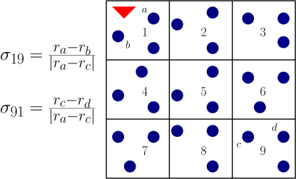
How does heterogeneity arise in practice? Our definition of heterogeneity is motivated by scenarios where the partitioning of arms into disjoint arm-sets is not arbitrary, but rather adheres to some structure. Consider for instance the target detection application we discussed in the Introduction; see Fig. 2 for an illustration. For this setting, sensors closer to the target have higher readings than those farther away. As a result, one should expect the readings of sensor to be more similar to those of sensor (in the same sub-region) as compared to those of sensor in sub-region 9. This spatial heterogeneity effect is precisely captured by low values of the arm-heterogeneity index One can similarly argue that spatial heterogeneity leads to low values of .
4.2 Main Result and Discussion
Our first main result, Theorem 1, shows that Fed-SEL is -PAC, and provides a detailed characterization of its sample- and communication-complexity. To state the result cleanly, we will use as a shorthand for , and employ the following notations:
Thus, is the difference in the mean rewards of the two best arms in . We remind the reader here that the best arm belongs to the arm-set of client .
Theorem 1.
Suppose Fed-SEL is run with . Then with probability at least , the following statements hold.
-
•
(Consistency) Fed-SEL terminates in finite-time and outputs the globally best arm, i.e., we have .
-
•
(Communication-Complexity) The number of rounds a client remains active during Phase II is bounded above as follows: , where
(5) and if . Similarly,
(6) and if . The number of communication rounds during Phase II is then given by ; client always remains active till Fed-SEL terminates, i.e., . Moreover, each client transmits at most
bits of information in each round .
-
•
(Sample-Complexity) The total number of arm-pulls made by client is bounded above by
(7)
Since each client can only sample arms from its own arm-set, it is apparent that at least one round of communication is necessary for solving Problem 1, in general. The next result - an immediate corollary of Theorem 1 - identifies heterogeneous regimes where one round of communication is also sufficient.888When , we would ideally like the upper-bound on to evaluate to . Setting in (5) causes the first two dominant terms in the upper-bound for to vanish, as desired. The lower order term that remains is an artifact of our analysis.
Corollary 1.
Suppose Fed-SEL is run with . Additionally, suppose
Then, with probability at least , Fed-SEL terminates after just one round of communication between the clients and the server, and outputs the globally best arm, i.e., .
The proof of Theorem 1 is deferred to Appendix A. In what follows, we discuss several important implications of Theorem 1.
(Benefit of Heterogeneity) From the first two dominant terms in the expressions for and in equations (5) and (6), respectively, observe that lower values of the arm-heterogeneity indices translate to fewer communication rounds. Moreover, fewer rounds imply fewer arm-pulls (and hence, lower sample-complexity) during Phase II, as is evident from Eq. (7). Since low values of arm-heterogeneity indices correspond to high heterogeneity, we conclude that heterogeneity helps reduce both the sample- and communication-complexity of Fed-SEL.
(Benefit of Local Steps) Even if the level of heterogeneity is low in a given instance, one can reduce the number of communication rounds of Fed-SEL by increasing the communication period ; see equations (5) and (6). Based on these equations and (7), we note that shows up as an additive term in the upper-bound on the number of arm-pulls made during Phase II. The key implication of this fact is that one can ramp up to significantly reduce communication and get away with a modest price in terms of additional sample-complexity. The main underlying reason for this stems from the observation that with Fed-SEL, more local steps always help by providing better arm-mean estimates.
(Benefit of Collaboration) We have already discussed how heterogeneity assists in reducing the sample-complexity of Phase II. To focus on the number of arm-pulls made by a client during Phase I, let us now turn our attention to the first term in Eq. (7). The summation in this term is over the local arm-set of client , as opposed to the global arm-set . Since can be much smaller than in practice, the benefit of collaboration is immediate: each client needs to explore only a small subset of the global arm-set, i.e., the task of exploration is distributed among clients.
(Number of Bits Exchanged) Since is the gap in mean rewards of the two best arms (i.e., the two arms that are hardest to distinguish) in the global arm set , the quantity essentially captures the complexity of a given instance of the MAB problem. Intuitively, one should expect that the amount of information that needs to be exchanged to solve a given instance of Problem 1 should scale with the complexity of that instance, i.e., with . From Theorem 1, we note that our adaptive encoding strategy formalizes this intuition to a certain extent.
Remark 3.
From the above discussion, note that although our algorithm itself is oblivious to both the level of heterogeneity and the complexity of a given instance, the sample- and communication-complexity bounds we obtain naturally adapt to these defining features of the instance, i.e., our guarantees are instance-dependent.
We now briefly comment on the main steps in the proof of Theorem 1.
Proof Sketch for Theorem 1: We first define a “good event” with measure at least , on which, the empirical means of all arms are within their respective confidence intervals at all times. On this event , we show using standard arguments that at the end of Phase I, each client successfully identifies the locally best arm in , i.e., . At this stage, to exploit heterogeneity, we require the locally best arm from each arm-set to be “well-explored”. Accordingly, we establish that , where is the flexible design parameter in line 1 of Algo. 1. The next key piece of our analysis pertains to relating the amount of exploration that has already been done during Phase I, to that which remains to be done during Phase II for eliminating all arms in the set ; this is precisely where the arm-heterogeneity indices show up in the analysis. To complete the above step, we derive new upper and lower bounds on the Lambert function that may be of independent interest; see Lemma 5 in Appendix A.1.
Before moving on to the next section, we discuss how certain aspects of our algorithm and analysis can be potentially improved.
Potential Refinements: As is most often the case, there is considerable room for improvement. First, the dependence on the number of arms within the logarithmic terms of our sample-complexity bounds can be improved using a variant of the Median Elimination Algorithm [13]. Second, note from (7) that for each client , its sample-complexity during Phase I scales inversely with the local arm-gaps , where , and is the locally best-arm in . Ideally, however, we would like to achieve sample-complexity bounds that scale inversely with , where is the globally best arm. For all clients other than client 1 (i.e., clients who cannot sample arm directly), this would necessarily require communication via the server. Thus, while we save on communication during Phase I, the price paid for doing so is a larger sample-complexity.
One may thus consider the alternative of merging Phases I and II. Our reasons, however, for persisting with separate phases are as follows. First, in our current approach, a client starts communicating when the best arm in its arm-set has already been well-explored. This, in turn, considerably reduces the workload for Phase II, and helps reduce communication significantly (see Corollary 1 for instance). The second important reason is somewhat more subtle: as we explain in the next section, having two separate phases aids the task of tolerating adversarial clients.
5 Robust Federated Best-Arm Identification
In this section, we will focus on the following question: Can we still hope to identify the best-arm when certain clients act adversarially? To formally answer this question, we will consider a Byzantine adversary model [81, 82] where adversarial clients have complete knowledge of the model, can collude among themselves, and act arbitrarily. Let us start by building some intuition. Suppose the client associated with the arm-set containing the globally best arm is adversarial. Since this is the only client that can sample , there is not much hope of identifying the best arm in this case. This simple observation reveals the need for information-redundancy: we need multiple clients to sample each arm-set to account for adversarial behaviour. Accordingly, with each arm-set , we now associate a group of clients ; thus, .999From now on, we will use the index to refer to arm-sets and client-groups, and the index to refer to clients. We will denote the set of honest clients by , the set of adversarial clients by , and allow at most clients to be adversarial in each client-group, i.e., . We will also assume that the server knows .
Simply restricting the number of adversaries in each client-group is not enough to identify the best arm; there are additional challenges that need to be dealt with. To see this, consider a scenario where an arm has not been adequately explored by an honest client . Due to the stochastic nature of our model, client , although honest, may have a poor estimate of arm true mean reward at this stage. How can we distinguish this scenario from one where an adversarial client in deliberately transmits a completely incorrect estimate of arm ? In this context, one natural idea is to enforce each honest client to start transmitting information only when it has sufficiently explored every arm in its arm-set. This further justifies the rationale behind having two separate phases in Fed-SEL. In what follows, we describe a robust variant of Fed-SEL.
Description of Robust Fed-SEL: To identify despite adversaries, we propose Robust Fed-SEL, and outline its main steps in Algorithm 3. Like the Fed-SEL algorithm, Robust Fed-SEL also involves two separate phases. During Phase I, in each client group , every honest client independently runs Algo. 1 on , and then transmits to the server exactly as in Fed-SEL. The key operations performed by the server as follows.
1) Majority Voting to Identify Representative Arms: At the onset of Phase II, the server waits till it has heard from at least clients of each client group before it starts acting. Next, for each arm-set , the server aims to compute a representative locally best arm . Note that adversarial clients in may collude and decide to report an arm to the server that has true mean much lower than that of the locally best arm in . Nonetheless, we should expect every honest client to output with high probability. Thus, if honest clients are in majority in , a simple majority voting operation (denoted by Maj_Vot) at the server should suffice to reveal the best arm in with high probability; this is precisely the rationale behind line 2. During the remainder of Phase II, for each client group , the server only uses the information of the subset of clients who reported the representative arm .
2) Trimming to Compute Robust Arm-Statistics: Phase II involves periodic communication and evolves in rounds. In each round , the server maintains a set of active client-groups: group is deemed active if is still under contention for being the globally best arm. To decide whether group should remain active, the server performs certain trimming operations that we next describe. Given a non-negative integer , and a set of scalars where , let denote the operation of removing the highest and lowest numbers from , and then returning any one of the remaining numbers. Based on this Trim operator, the server computes robust upper and lower estimates, namely and , of the mean of the representative arm ; see line 6.101010The trimming parameter is set based on the observation that clients in who report an arm other than are adversarial with high probability. Using these robust estimates, the server subsequently updates the set of active client-groups by executing lines 7-8.
If group remains active, then the server needs more refined arm estimates of arm from . Accordingly, the server sends out a binary vector that encodes the active client-groups: if and only if . Upon receiving , each honest client in checks if . If so, it samples arm times, encodes as in Fed-SEL, and transmits the encoding to the server. If is not received from the server, or if , client does nothing further. This completes the description of Robust Fed-SEL.
Comments on Algorithm 3: Before providing formal guarantees for Robust Fed-SEL, a few comments are in order. First, note that unlike Fed-SEL where the server transmitted a threshold to enable the clients to figure out whether they are active or not, the server instead transmits a vector in Robust Fed-SEL. The reason for this is as follows. Even if for some client-group , it may very well be that for some Thus, even if the server is able to eliminate client group on its end, simply broadcasting the threshold may not be enough for every client in to realize that it no longer needs to sample arm . Note that for line 10 of Robust Fed-SEL to make sense, we assume that every client is aware of the client-group to which it belongs.
During Phase II, for each group , since the server only uses the information of clients in , we have not explicitly specified actions for honest clients in to avoid cluttering the exposition. A potential specification is as follows. Suppose the first time an honest client hears from the server, it is still in the process of completing Phase I. Since in this case client cannot belong to , it deactivates and does nothing further. In all other cases, client acts exactly as specified in line 10 of Robust Fed-SEL.
The main result of this section is as follows.
Theorem 2.
Suppose and . Then, Robust Fed-SEL is -PAC.
Discussion: Under information-redundancy, i.e., under the condition that “enough” clients sample every arm in each arm-set (), Theorem 2 shows that Robust Fed-SEL is an adversarially-robust -PAC algorithm. Despite the flurry of research on tolerating adversaries in distributed optimization/supervised learning [26, 27, 28, 29, 30, 31, 32, 33, 34, 35], there is no analogous result (that we know of) in the context of MAB problems. Theorem 2 fills this gap. The sample- and communication-complexity bounds for Robust Fed-SEL are of the same order as that of Fed-SEL; hence, we do not explicitly state them here. For a discussion on this topic, see Appendix B where we provide the proof of Theorem 2.
Remark 4.
The type of redundancy assumption we make in Theorem 2 is extremely standard in the literature on tolerating worst-case adversarial models. Similar assumptions are made in [26, 27, 28, 29, 30, 31, 32, 33, 34, 35] where typically less than half of the agents (clients) are allowed to be adversarial. The reason why we allow at most of the clients in each client-group to be adversarial (as opposed to at most ) is because some adversaries may choose not to transmit anything at all. In this case, the server may never acquire enough information from to compute . Now consider a slightly weaker adversary model where every client transmits when it is supposed to, but the information being sent can be arbitrarily corrupted for clients under attack. For this setting, our results go through identically under the weaker assumption that and .
We now investigate how the ideas developed herein can be extended to the peer-to-peer setting.
6 Robust Peer-to-Peer Best-Arm Identification
In this section, we consider the challenging setting of best-arm identification over a fully-distributed network in the presence of adversarial clients. Formally, the network is described by a static directed graph , where the vertex set is composed of the set of clients, i.e., , and represents the set of edges between them. An edge indicates that client can directly transmit information to client . The set of all in-neighbors (resp., out-neighbors) of client is defined as (resp., ).
Our goal is to design a distributed algorithm that ensures that each honest client can eventually identify the globally best arm , despite the actions of the adversarial clients . Clearly, we need some upper-bound on the number of adversaries for the problem to make sense. To this end, we will consider an -local Byzantine adversary model [83, 84, 85, 86] where there are at most adversarial clients in the in-neighborhood of each honest client, i.e., . Recall that clients in can only sample arms from . Thus, to acquire information about some other arm-set (say), we need information to diffuse from the clients in to clients in . If there is a small cut (bottleneck) in the graph separating from , then such a cut can be infested by adversaries, thereby preventing the flow of information necessary for identifying . From this intuitive reasoning, note that we need sufficient disjoint paths linking different client groups to have any hope of tackling adversaries. The key graph-theoretic property that we will exploit in this context is a notion of strong-robustness [86] adapted to our setting.
Definition 2.
(Strong-robustness w.r.t. ) Given any positive integer , the graph is said to be strongly -robust w.r.t. the client group if every non-empty subset contains at least one client with in-neighbors outside , i.e., for every non-empty set , such that .
We note that if is strongly -robust w.r.t. , then (follows by considering ). Thus, the above definition implicitly captures information-redundancy. At the same time, it ensures that there is adequate redundancy in the network-structure to reliably disseminate information about arm-set from to the rest of the network. We now develop an algorithm, namely Algorithm 4, that leverages the strong-robustness property in Definition 2.
Description of Algorithm 4: Each client maintains two -dimensional vectors and . The -th entry of , namely , stores client ’s estimate of the locally best arm in arm-set , and stores an estimate of the corresponding arm’s mean. Consider a client . Since client can sample all arms in , it updates and on its own by running Algo. 1 on . To learn about the best arm in all arm-sets other than , client needs to interact with its neighbors, some of whom might be adversarial. For each , the strategy employed by client to update and is very similar to that of the server in Robust Fed-SEL. In short, collects information about from its neighbors, performs majority voting to decide (line 3), and does a trimming operation to compute (line 4). For this operation, client only uses the estimates of those neighbors that report the majority-voted arm . Once all components of and have been populated, client executes line 5 to identify the globally best arm.
We now present the main result of this section.
Theorem 3.
Suppose the following arm-heterogeneity condition holds:
| (8) |
Moreover, suppose the adversary model is -local, and is strongly -robust w.r.t. . Then, with probability at least , Algorithm 4 terminates in finite-time, and outputs .
Discussion: The above result is the only one we know of that provides any guarantees against adversarial attacks for MAB problems over general networks. While the strong-robustness property in Definition 2 has been exploited earlier in the context of resilient distributed state estimation [86] and hypothesis-testing/inference [87], Theorem 3 reveals that the same graph-theoretic property ends up playing a crucial role for the best-arm identification problem we consider here.111111By making a connection to bootstrap percolation theory, the authors in [86] show that the strong-robustness property in Definition 2 can be checked in polynomial time.
To isolate the subtleties and challenges associated with tolerating adversaries over a general network, we worked under an arm-heterogeneity assumption. This assumption effectively bypasses the need for Phase II, i.e., the sample-complexity of a client is given by the number of arm-pulls it makes during Phase I. We believe that the ideas presented in this paper can be extended in an appropriate way to study the networked setting without making the arm-heterogeneity assumption.
7 Simulations
In this section, we verify some of our theoretical findings based on a simple simulation example. Motivated by distributed target tracking applications in cooperative learning [20, 21, 22, 23], we consider a target detection problem involving 9 static sensors distributed over an environment. The environment is divided into 3 sub-regions with 3 sensors and a mobile robot in each sub-region. Each mobile robot can access the sensor readings of the sensors in its sub-region, and transmit information to a central controller. The goal is to detect a static target located in one of the sub-regions. We model this setting by mapping sensors to arms, sub-regions to arm-sets, and robots to clients. Each sensor displays binary readings: sensors that are located closer to the target have a higher probability of displaying . Thus, finding the “best arm” in this setting corresponds to localizing the target, and a robot visiting a sensor corresponds to a client sampling an arm. Ideally, to minimize battery life of the robots, we would like to locate the target with a small number of visits (sample-complexity), and only a few information exchanges with the controller (communication-complexity).
We assume the target is located in the first sub-region that corresponds to arm-set . Arm rewards (sensor readings) are drawn from Bernoulli distributions with means , , and associated with the arm-sets (sub-regions) , and , respectively. Based on the definition of arm-heterogeneity indices in Definition 1, the parameter captures the level of heterogeneity in the example we have described above. In particular, it is easy to verify that for each ,
| (9) |
 |
 |
| (a) | (b) |
For the example we have considered, arm-heterogeneity has a very natural spatial interpretation: sensors located closer to the target output higher readings than those farther away. Note that arm 1 in is the best arm, and hence closest to the target. With confidence parameter , we implement a simplified version of Fed-SEL (Algo. 2) without any adaptive quantization. We vary the level of heterogeneity by tuning , and for each value of , perform trials.
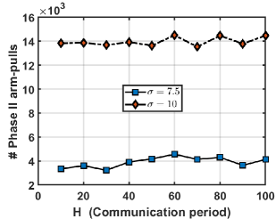
Main Observations: Below, we discuss our experimental findings from Figure 4.
-
•
From Fig. 4(a), we note a distinct trend: the number of communication rounds decrease with an increase in the level of arm-heterogeneity , exactly as suggested by Theorem 1. Moreover, when , Fed-SEL terminates in 1 round, complying with Corollary 1. We conclude that Fed-SEL does indeed benefit from the notion of heterogeneity that we have introduced.
-
•
From Fig. 4(a), we note that doubling the communication period roughly halves the number of communication rounds, as expected. Importantly, increasing the communication period does not cause the number of arm-pulls in Phase II to increase much; see Fig. 4(b). These observations once again align with our theoretical findings in Theorem 1: since local computations always help for Fed-SEL, one can significantly reduce communication by increasing , and at the same time, not pay much of an additional price in terms of sample-complexity.
8 Conclusion and Future Work
We introduced and studied the federated best-arm identification problem where clients with disjoint arm-sets collaborate via a server to identify the globally best arm with the highest mean pay-off. We defined a novel notion of arm-heterogeneity for this problem, and proved that when such heterogeneity is exploited in a principled way, one can significantly reduce the number of communication rounds required to identify the best arm (with high probability). Our finding is unique in that it reveals that unlike federated supervised learning, heterogeneity can provably help for best-arm identification problems in stochastic multi-armed bandits. Finally, a key advantage of our algorithmic approach is that it is robust to worst-case adversarial actions.
There are several interesting avenues of future research, as we discuss below.
-
•
First, we aim to derive lower-bounds on the sample-complexity for the problem we have introduced. This will shed light on the tightness of our results in Theorem 1, and inform the need for potentially better algorithms. It would also be interesting to explore alternate formulations where the communication budget is fixed a priori, and the goal is to maximize the probability of identifying the best arm subject to such a budget.
-
•
Perhaps the most interesting direction is to see if the ideas developed in this paper have immediate extensions to general Markov decision processes (MDP’s) in the context of reinforcement learning. Specifically, we wish to investigate the trade-offs between communication-complexity and performance measures such as PAC bounds or regret for distributed sequential decision-making problems.
-
•
Another important direction is to explore related settings where statistical heterogeneity can provably help. Our conjecture is that for problems where the globally optimal parameter belongs to a finite set, one can establish results similar to those in this paper by using elimination-based techniques. In this context, one ripe candidate problem is that of hypothesis-testing/statistical inference where the true hypothesis belongs to a finite set of possible hypotheses. Recent results have shown that for peer-to-peer versions of this problem [88, 89], one can design principled approaches to significantly reduce communication.
-
•
Some recent works have shown that by either considering alternate problem formulations (such as personalized variants of FL [90, 91, 92, 93]), or by drawing on ideas from representation learning [94], one can train meaningful statistical models in FL, despite statistical heterogeneity. It may be worthwhile to investigate whether such ideas apply to the setting we consider. Finally, while we studied robustness to adversarial actions, it would also be interesting to explore robustness to other challenges, such as distribution shifts [95], or stragglers [96, 97, 80].
References
- [1] Jakub Konečnỳ, H Brendan McMahan, Felix X Yu, Peter Richtárik, Ananda Theertha Suresh, and Dave Bacon. Federated learning: Strategies for improving communication efficiency. arXiv preprint arXiv:1610.05492, 2016.
- [2] Brendan McMahan, Eider Moore, Daniel Ramage, Seth Hampson, and Blaise Aguera y Arcas. Communication-efficient learning of deep networks from decentralized data. In Artificial Intelligence and Statistics, pages 1273–1282. PMLR, 2017.
- [3] Keith Bonawitz, Hubert Eichner, Wolfgang Grieskamp, Dzmitry Huba, Alex Ingerman, Vladimir Ivanov, Chloe Kiddon, Jakub Konečnỳ, Stefano Mazzocchi, H Brendan McMahan, et al. Towards federated learning at scale: System design. arXiv preprint arXiv:1902.01046, 2019.
- [4] Peter Kairouz, H Brendan McMahan, Brendan Avent, Aurélien Bellet, Mehdi Bennis, Arjun Nitin Bhagoji, Keith Bonawitz, Zachary Charles, Graham Cormode, Rachel Cummings, et al. Advances and open problems in federated learning. arXiv preprint arXiv:1912.04977, 2019.
- [5] Tian Li, Anit Kumar Sahu, Ameet Talwalkar, and Virginia Smith. Federated learning: Challenges, methods, and future directions. IEEE Signal Processing Magazine, 37(3):50–60, 2020.
- [6] Xiang Li, Kaixuan Huang, Wenhao Yang, Shusen Wang, and Zhihua Zhang. On the convergence of fedavg on non-iid data. arXiv preprint arXiv:1907.02189, 2019.
- [7] Grigory Malinovskiy, Dmitry Kovalev, Elnur Gasanov, Laurent Condat, and Peter Richtarik. From local sgd to local fixed-point methods for federated learning. In International Conference on Machine Learning, pages 6692–6701. PMLR, 2020.
- [8] Zachary Charles and Jakub Konečnỳ. On the outsized importance of learning rates in local update methods. arXiv preprint arXiv:2007.00878, 2020.
- [9] Zachary Charles and Jakub Konečnỳ. Convergence and accuracy trade-offs in federated learning and meta-learning. In International Conference on Artificial Intelligence and Statistics, pages 2575–2583. PMLR, 2021.
- [10] Reese Pathak and Martin J Wainwright. Fedsplit: An algorithmic framework for fast federated optimization. arXiv preprint arXiv:2005.05238, 2020.
- [11] Sai Praneeth Karimireddy, Satyen Kale, Mehryar Mohri, Sashank Reddi, Sebastian Stich, and Ananda Theertha Suresh. Scaffold: Stochastic controlled averaging for federated learning. In International Conference on Machine Learning, pages 5132–5143. PMLR, 2020.
- [12] Don Kurian Dennis, Tian Li, and Virginia Smith. Heterogeneity for the win: One-shot federated clustering. arXiv preprint arXiv:2103.00697, 2021.
- [13] Eyal Even-Dar, Shie Mannor, and Yishay Mansour. Pac bounds for multi-armed bandit and markov decision processes. In International Conference on Computational Learning Theory, pages 255–270. Springer, 2002.
- [14] Eyal Even-Dar, Shie Mannor, Yishay Mansour, and Sridhar Mahadevan. Action elimination and stopping conditions for the multi-armed bandit and reinforcement learning problems. Journal of machine learning research, 7(6), 2006.
- [15] Kevin Jamieson, Matthew Malloy, Robert Nowak, and Sébastien Bubeck. lil’ucb: An optimal exploration algorithm for multi-armed bandits. In Conference on Learning Theory, pages 423–439. PMLR, 2014.
- [16] Jean-Yves Audibert, Sébastien Bubeck, and Rémi Munos. Best arm identification in multi-armed bandits. In COLT, pages 41–53, 2010.
- [17] Sébastien Bubeck, Rémi Munos, and Gilles Stoltz. Pure exploration in finitely-armed and continuous-armed bandits. Theoretical Computer Science, 412(19):1832–1852, 2011.
- [18] Victor Gabillon, Mohammad Ghavamzadeh, and Alessandro Lazaric. Best arm identification: A unified approach to fixed budget and fixed confidence. In NIPS-Twenty-Sixth Annual Conference on Neural Information Processing Systems, 2012.
- [19] Kevin Jamieson and Robert Nowak. Best-arm identification algorithms for multi-armed bandits in the fixed confidence setting. In 2014 48th Annual Conference on Information Sciences and Systems (CISS), pages 1–6. IEEE, 2014.
- [20] Volkan Cevher, Marco F Duarte, and Richard G Baraniuk. Distributed target localization via spatial sparsity. In 2008 16th European Signal Processing Conference, pages 1–5. IEEE, 2008.
- [21] Antonio Franchi, Paolo Stegagno, Maurizio Di Rocco, and Giuseppe Oriolo. Distributed target localization and encirclement with a multi-robot system. IFAC Proceedings Volumes, 43(16):151–156, 2010.
- [22] Vladimir Savic, Henk Wymeersch, and Santiago Zazo. Belief consensus algorithms for fast distributed target tracking in wireless sensor networks. Signal Processing, 95:149–160, 2014.
- [23] Philip Dames, Pratap Tokekar, and Vijay Kumar. Detecting, localizing, and tracking an unknown number of moving targets using a team of mobile robots. The International Journal of Robotics Research, 36(13-14):1540–1553, 2017.
- [24] Shahin Shahrampour, Alexander Rakhlin, and Ali Jadbabaie. Distributed detection: Finite-time analysis and impact of network topology. IEEE Transactions on Automatic Control, 61(11):3256–3268, 2015.
- [25] Robert M Corless, Gaston H Gonnet, David EG Hare, David J Jeffrey, and Donald E Knuth. On the lambertw function. Advances in Computational mathematics, 5(1):329–359, 1996.
- [26] Yudong Chen, Lili Su, and Jiaming Xu. Distributed statistical machine learning in adversarial settings: Byzantine gradient descent. Proceedings of the ACM on Measurement and Analysis of Computing Systems, 1(2):1–25, 2017.
- [27] Peva Blanchard, El Mahdi El Mhamdi, Rachid Guerraoui, and Julien Stainer. Machine learning with adversaries: Byzantine tolerant gradient descent. In Proceedings of the 31st International Conference on Neural Information Processing Systems, pages 118–128, 2017.
- [28] Dong Yin, Yudong Chen, Ramchandran Kannan, and Peter Bartlett. Byzantine-robust distributed learning: Towards optimal statistical rates. In International Conference on Machine Learning, pages 5650–5659. PMLR, 2018.
- [29] Lingjiao Chen, Zachary Charles, Dimitris Papailiopoulos, et al. Draco: Robust distributed training via redundant gradients. arXiv preprint arXiv:1803.09877, 2018.
- [30] Dan Alistarh, Zeyuan Allen-Zhu, and Jerry Li. Byzantine stochastic gradient descent. arXiv preprint arXiv:1803.08917, 2018.
- [31] Cong Xie, Oluwasanmi Koyejo, and Indranil Gupta. Generalized byzantine-tolerant sgd. arXiv preprint arXiv:1802.10116, 2018.
- [32] Liping Li, Wei Xu, Tianyi Chen, Georgios B Giannakis, and Qing Ling. Rsa: Byzantine-robust stochastic aggregation methods for distributed learning from heterogeneous datasets. In Proceedings of the AAAI Conference on Artificial Intelligence, volume 33, pages 1544–1551, 2019.
- [33] Avishek Ghosh, Justin Hong, Dong Yin, and Kannan Ramchandran. Robust federated learning in a heterogeneous environment. arXiv preprint arXiv:1906.06629, 2019.
- [34] Avishek Ghosh, Raj Kumar Maity, Swanand Kadhe, Arya Mazumdar, and Kannan Ramachandran. Communication efficient and byzantine tolerant distributed learning. In 2020 IEEE International Symposium on Information Theory (ISIT), pages 2545–2550. IEEE, 2020.
- [35] Avishek Ghosh, Raj Kumar Maity, and Arya Mazumdar. Distributed newton can communicate less and resist byzantine workers. arXiv preprint arXiv:2006.08737, 2020.
- [36] Eshcar Hillel, Zohar Karnin, Tomer Koren, Ronny Lempel, and Oren Somekh. Distributed exploration in multi-armed bandits. arXiv preprint arXiv:1311.0800, 2013.
- [37] Chao Tao, Qin Zhang, and Yuan Zhou. Collaborative learning with limited interaction: Tight bounds for distributed exploration in multi-armed bandits. In 2019 IEEE 60th Annual Symposium on Foundations of Computer Science (FOCS), pages 126–146. IEEE, 2019.
- [38] Keqin Liu and Qing Zhao. Distributed learning in multi-armed bandit with multiple players. IEEE Transactions on Signal Processing, 58(11):5667–5681, 2010.
- [39] Dileep Kalathil, Naumaan Nayyar, and Rahul Jain. Decentralized learning for multiplayer multiarmed bandits. IEEE Transactions on Information Theory, 60(4):2331–2345, 2014.
- [40] Soummya Kar, H Vincent Poor, and Shuguang Cui. Bandit problems in networks: Asymptotically efficient distributed allocation rules. In 2011 50th IEEE Conference on Decision and Control and European Control Conference, pages 1771–1778. IEEE, 2011.
- [41] Peter Landgren, Vaibhav Srivastava, and Naomi Ehrich Leonard. Distributed cooperative decision-making in multiarmed bandits: Frequentist and bayesian algorithms. In 2016 IEEE 55th Conference on Decision and Control (CDC), pages 167–172. IEEE, 2016.
- [42] Peter Landgren, Vaibhav Srivastava, and Naomi Ehrich Leonard. Distributed cooperative decision making in multi-agent multi-armed bandits. Automatica, 125:109445, 2021.
- [43] Shahin Shahrampour, Alexander Rakhlin, and Ali Jadbabaie. Multi-armed bandits in multi-agent networks. In 2017 IEEE International Conference on Acoustics, Speech and Signal Processing (ICASSP), pages 2786–2790. IEEE, 2017.
- [44] Swapna Buccapatnam, Jian Tan, and Li Zhang. Information sharing in distributed stochastic bandits. In 2015 IEEE Conference on Computer Communications (INFOCOM), pages 2605–2613. IEEE, 2015.
- [45] Ravi Kumar Kolla, Krishna Jagannathan, and Aditya Gopalan. Collaborative learning of stochastic bandits over a social network. IEEE/ACM Transactions on Networking, 26(4):1782–1795, 2018.
- [46] Yuanhao Wang, Jiachen Hu, Xiaoyu Chen, and Liwei Wang. Distributed bandit learning: Near-optimal regret with efficient communication. arXiv preprint arXiv:1904.06309, 2019.
- [47] Abishek Sankararaman, Ayalvadi Ganesh, and Sanjay Shakkottai. Social learning in multi agent multi armed bandits. Proceedings of the ACM on Measurement and Analysis of Computing Systems, 3(3):1–35, 2019.
- [48] David Martínez-Rubio, Varun Kanade, and Patrick Rebeschini. Decentralized cooperative stochastic bandits. arXiv preprint arXiv:1810.04468, 2018.
- [49] Abhimanyu Dubey et al. Kernel methods for cooperative multi-agent contextual bandits. In International Conference on Machine Learning, pages 2740–2750. PMLR, 2020.
- [50] Abhimanyu Dubey and Alex Pentland. Differentially-private federated linear bandits. arXiv preprint arXiv:2010.11425, 2020.
- [51] Anusha Lalitha and Andrea Goldsmith. Bayesian algorithms for decentralized stochastic bandits. arXiv preprint arXiv:2010.10569, 2020.
- [52] Ronshee Chawla, Abishek Sankararaman, Ayalvadi Ganesh, and Sanjay Shakkottai. The gossiping insert-eliminate algorithm for multi-agent bandits. In International Conference on Artificial Intelligence and Statistics, pages 3471–3481. PMLR, 2020.
- [53] Ronshee Chawla, Abishek Sankararaman, and Sanjay Shakkottai. Multi-agent low-dimensional linear bandits. arXiv preprint arXiv:2007.01442, 2020.
- [54] Avishek Ghosh, Abishek Sankararaman, and Kannan Ramchandran. Collaborative learning and personalization in multi-agent stochastic linear bandits. arXiv preprint arXiv:2106.08902, 2021.
- [55] Mridul Agarwal, Vaneet Aggarwal, and Kamyar Azizzadenesheli. Multi-agent multi-armed bandits with limited communication. arXiv preprint arXiv:2102.08462, 2021.
- [56] Zhaowei Zhu, Jingxuan Zhu, Ji Liu, and Yang Liu. Federated bandit: A gossiping approach. In Abstract Proceedings of the 2021 ACM SIGMETRICS/International Conference on Measurement and Modeling of Computer Systems, pages 3–4, 2021.
- [57] Chengshuai Shi, Cong Shen, and Jing Yang. Federated multi-armed bandits with personalization. In International Conference on Artificial Intelligence and Statistics, pages 2917–2925. PMLR, 2021.
- [58] Kwang-Sung Jun, Lihong Li, Yuzhe Ma, and Xiaojin Zhu. Adversarial attacks on stochastic bandits. arXiv preprint arXiv:1810.12188, 2018.
- [59] Fang Liu and Ness Shroff. Data poisoning attacks on stochastic bandits. In International Conference on Machine Learning, pages 4042–4050. PMLR, 2019.
- [60] Thodoris Lykouris, Vahab Mirrokni, and Renato Paes Leme. Stochastic bandits robust to adversarial corruptions. In Proceedings of the 50th Annual ACM SIGACT Symposium on Theory of Computing, pages 114–122, 2018.
- [61] Anupam Gupta, Tomer Koren, and Kunal Talwar. Better algorithms for stochastic bandits with adversarial corruptions. In Conference on Learning Theory, pages 1562–1578. PMLR, 2019.
- [62] Ilija Bogunovic, Andreas Krause, and Jonathan Scarlett. Corruption-tolerant gaussian process bandit optimization. In International Conference on Artificial Intelligence and Statistics, pages 1071–1081. PMLR, 2020.
- [63] Evrard Garcelon, Baptiste Roziere, Laurent Meunier, Jean Tarbouriech, Olivier Teytaud, Alessandro Lazaric, and Matteo Pirotta. Adversarial attacks on linear contextual bandits. arXiv preprint arXiv:2002.03839, 2020.
- [64] Ilija Bogunovic, Arpan Losalka, Andreas Krause, and Jonathan Scarlett. Stochastic linear bandits robust to adversarial attacks. In International Conference on Artificial Intelligence and Statistics, pages 991–999. PMLR, 2021.
- [65] Daniel Vial, Sanjay Shakkottai, and R Srikant. Robust multi-agent multi-armed bandits. In Proceedings of the Twenty-second International Symposium on Theory, Algorithmic Foundations, and Protocol Design for Mobile Networks and Mobile Computing, pages 161–170, 2021.
- [66] Sebastian U Stich. Local sgd converges fast and communicates little. arXiv preprint arXiv:1805.09767, 2018.
- [67] Jianyu Wang and Gauri Joshi. Cooperative sgd: A unified framework for the design and analysis of communication-efficient sgd algorithms. arXiv preprint arXiv:1808.07576, 2018.
- [68] Artin Spiridonoff, Alex Olshevsky, and Ioannis Ch Paschalidis. Local sgd with a communication overhead depending only on the number of workers. arXiv preprint arXiv:2006.02582, 2020.
- [69] Amirhossein Reisizadeh, Aryan Mokhtari, Hamed Hassani, Ali Jadbabaie, and Ramtin Pedarsani. Fedpaq: A communication-efficient federated learning method with periodic averaging and quantization. In International Conference on Artificial Intelligence and Statistics, pages 2021–2031. PMLR, 2020.
- [70] Farzin Haddadpour, Mohammad Mahdi Kamani, Mehrdad Mahdavi, and Viveck Cadambe. Local sgd with periodic averaging: Tighter analysis and adaptive synchronization. In Advances in Neural Information Processing Systems, pages 11082–11094, 2019.
- [71] Farzin Haddadpour, Mohammad Mahdi Kamani, Aryan Mokhtari, and Mehrdad Mahdavi. Federated learning with compression: Unified analysis and sharp guarantees. In International Conference on Artificial Intelligence and Statistics, pages 2350–2358. PMLR, 2021.
- [72] Blake Woodworth, Kumar Kshitij Patel, Sebastian U Stich, Zhen Dai, Brian Bullins, H Brendan McMahan, Ohad Shamir, and Nathan Srebro. Is local sgd better than minibatch sgd? arXiv preprint arXiv:2002.07839, 2020.
- [73] Ahmed Khaled, Konstantin Mishchenko, and Peter Richtárik. First analysis of local gd on heterogeneous data. arXiv preprint arXiv:1909.04715, 2019.
- [74] Ahmed Khaled, Konstantin Mishchenko, and Peter Richtárik. Tighter theory for local sgd on identical and heterogeneous data. In International Conference on Artificial Intelligence and Statistics, pages 4519–4529. PMLR, 2020.
- [75] Farzin Haddadpour and Mehrdad Mahdavi. On the convergence of local descent methods in federated learning. arXiv preprint arXiv:1910.14425, 2019.
- [76] Anastasia Koloskova, Nicolas Loizou, Sadra Boreiri, Martin Jaggi, and Sebastian U Stich. A unified theory of decentralized sgd with changing topology and local updates. arXiv preprint arXiv:2003.10422, 2020.
- [77] Anit Kumar Sahu, Tian Li, Maziar Sanjabi, Manzil Zaheer, Ameet Talwalkar, and Virginia Smith. On the convergence of federated optimization in heterogeneous networks. arXiv preprint arXiv:1812.06127, 3, 2018.
- [78] Jianyu Wang, Qinghua Liu, Hao Liang, Gauri Joshi, and H Vincent Poor. Tackling the objective inconsistency problem in heterogeneous federated optimization. arXiv preprint arXiv:2007.07481, 2020.
- [79] Eduard Gorbunov, Filip Hanzely, and Peter Richtárik. Local sgd: Unified theory and new efficient methods. In International Conference on Artificial Intelligence and Statistics, pages 3556–3564. PMLR, 2021.
- [80] Aritra Mitra, Rayana Jaafar, George J Pappas, and Hamed Hassani. Achieving linear convergence in federated learning under objective and systems heterogeneity. arXiv preprint arXiv:2102.07053, 2021.
- [81] Marshall Pease, Robert Shostak, and Leslie Lamport. Reaching agreement in the presence of faults. Journal of the ACM (JACM), 27(2):228–234, 1980.
- [82] Danny Dolev, Nancy A Lynch, Shlomit S Pinter, Eugene W Stark, and William E Weihl. Reaching approximate agreement in the presence of faults. Journal of the ACM (JACM), 33(3):499–516, 1986.
- [83] C.Y. Koo. Broadcast in radio networks tolerating Byzantine adversarial behavior. In Proc. of the ACM Symp. on Principles of Distributed Comp., pages 275–282. ACM, 2004.
- [84] A. Pelc and D. Peleg. Broadcasting with locally bounded Byzantine faults. Info. Proc. Letters, 93(3):109–115, 2005.
- [85] H. J. LeBlanc, H. Zhang, X. Koutsoukos, and S. Sundaram. Resilient asymptotic consensus in robust networks. IEEE Journal on Selected Areas in Comm., 31(4):766–781, 2013.
- [86] Aritra Mitra and Shreyas Sundaram. Byzantine-resilient distributed observers for LTI systems. Automatica, 108:108487, 2019.
- [87] Aritra Mitra, John A Richards, and Shreyas Sundaram. A new approach to distributed hypothesis testing and non-Bayesian learning: Improved learning rate and Byzantine-resilience. IEEE Transactions on Automatic Control, 2020.
- [88] Aritra Mitra, John A Richards, and Shreyas Sundaram. A communication-efficient algorithm for exponentially fast non-Bayesian learning in networks. In 2019 IEEE 58th Conference on Decision and Control (CDC), pages 8347–8352. IEEE, 2019.
- [89] Aritra Mitra, John A Richards, Saurabh Bagchi, and Shreyas Sundaram. Distributed inference with sparse and quantized communication. IEEE Transactions on Signal Processing, 2021.
- [90] Yihan Jiang, Jakub Konečnỳ, Keith Rush, and Sreeram Kannan. Improving federated learning personalization via model agnostic meta learning. arXiv preprint arXiv:1909.12488, 2019.
- [91] Sen Lin, Guang Yang, and Junshan Zhang. A collaborative learning framework via federated meta-learning. In 2020 IEEE 40th International Conference on Distributed Computing Systems (ICDCS), pages 289–299. IEEE, 2020.
- [92] Alireza Fallah, Aryan Mokhtari, and Asuman Ozdaglar. Personalized federated learning: A meta-learning approach. arXiv preprint arXiv:2002.07948, 2020.
- [93] Filip Hanzely, Slavomír Hanzely, Samuel Horváth, and Peter Richtárik. Lower bounds and optimal algorithms for personalized federated learning. arXiv preprint arXiv:2010.02372, 2020.
- [94] Liam Collins, Hamed Hassani, Aryan Mokhtari, and Sanjay Shakkottai. Exploiting shared representations for personalized federated learning. arXiv preprint arXiv:2102.07078, 2021.
- [95] Amirhossein Reisizadeh, Farzan Farnia, Ramtin Pedarsani, and Ali Jadbabaie. Robust federated learning: The case of affine distribution shifts. arXiv preprint arXiv:2006.08907, 2020.
- [96] Jianyu Wang, Qinghua Liu, Hao Liang, Gauri Joshi, and H Vincent Poor. Tackling the objective inconsistency problem in heterogeneous federated optimization. Advances in Neural Information Processing Systems, 33, 2020.
- [97] Amirhossein Reisizadeh, Isidoros Tziotis, Hamed Hassani, Aryan Mokhtari, and Ramtin Pedarsani. Straggler-resilient federated learning: Leveraging the interplay between statistical accuracy and system heterogeneity. arXiv preprint arXiv:2012.14453, 2020.
- [98] Wassily Hoeffding. Probability inequalities for sums of bounded random variables. In The Collected Works of Wassily Hoeffding, pages 409–426. Springer, 1994.
- [99] Ioannis Chatzigeorgiou. Bounds on the lambert function and their application to the outage analysis of user cooperation. IEEE Communications Letters, 17(8):1505–1508, 2013.
Appendix A Proof of Theorem 1
The goal of this section is to prove Theorem 1. Throughout the proof, to simplify notation, we will use as a shorthand to represent the best arm in arm-set . Also, for any arm , we will use to denote the number of pulls made to arm by client during the course of operation of Fed-SEL. Before diving into the formal argument, we first outline the main steps of the proof.
-
•
Step 1: The first step of our analysis is to define a “good event” , and show that it occurs with probability at least , where is the given confidence parameter. On this good event, the empirical estimates of all arms are within appropriate confidence intervals (as given by the ) of the true means. See Lemma 1.
- •
-
•
Step 3: The next key step of our analysis is to bound the error of each client ’s estimate of the true mean , at the end of Phase I, as a function of the local arm-gap . This analysis, carried out in Lemma 3, reveals that the locally best arm from each arm-set is “well-explored” at the end of Phase I.
-
•
Step 4: The final piece of the analysis is to relate the amount of exploration that has been done during Phase I, to that which remains to be done during Phase II, for eliminating each client in the set Specifically, for each client , we seek a lower bound on the number of times arm has been sampled during Phase I, and an upper bound on the number of times it still needs to be sampled during Phase II, before being deemed sub-optimal. See Lemma 4. To complete this step, we derive new bounds on the Lambert function in Lemma 5 of Appendix A.1. These bounds may be of independent interest.
We now proceed to establish each of the above steps, starting with Step 1.
Lemma 1.
Consider the event defined as follows:
| (10) |
Then, it holds that .
Proof.
We can assume that the sequence of rewards for each arm is drawn before the algorithm is initiated. That way, for any , the empirical estimate of the mean of an arm after pulls is well defined, even if it has not actually been pulled times by a client. Applying the union bound gives us
| (11) | ||||
The second step above follows from an application of Hoeffding’s inequality [98]. ∎
For Step 2, we have the following lemma.
Lemma 2.
Suppose Fed-SEL is run with , where . Then, on the event , for each client , Algo. 1 terminates in finite-time and outputs .
Proof.
We prove the result for the case when ; the same reasoning applies when . Fix a client . We first argue that on , the locally best arm in never gets eliminated when Algo. 1 is run. To see this, observe that on , the following holds in each epoch :
At the same time, for any other arm , the following also holds on :
Thus, on , we have that
From line 5 of Algo. 1, it is then clear that does not get eliminated on . We now argue that every arm eventually gets eliminated. In particular, we claim that
is a sufficient condition to eliminate arm . To see this, suppose the above condition holds. We then have
| (12) | ||||
The claim then follows from line 5 of Algo. 1. This completes the proof. ∎
The next lemma provides a bound on the confidence intervals at the end of Phase I.
Lemma 3.
Suppose Fed-SEL is run with , where . Then, on the event , the following holds for every client :
| (13) |
where .
Proof.
Fix a client . From Lemma 2, we know that every arm eventually gets eliminated when client runs Algo. 1 on . We split our subsequent analysis into two cases depending on when the second best arm in gets eliminated during Phase I.
Case 1: Suppose arm is eliminated in the last epoch . On event , the arm with the largest empirical mean in must be (from Lemma 2). Thus, we must have
| (14) | ||||
Case 2: Suppose arm is eliminated in some epoch . For this to happen on , it must be that . This is easy to verify. Moreover, note that there must exist some arm that does not get eliminated in epoch , but gets eliminated in epoch . Thus, the following inequalities must hold simultaneously:
| (15) |
implying . Since we are on , this further implies that
| (16) |
At the same time, since arm gets eliminated in epoch , we must also have
| (17) |
following the analysis of Case 1. Combining Eq. (16) with the above bound yields
| (18) | ||||
Finally, since arm gets eliminated in the last epoch , an argument identical to the Case 1 analysis reveals that
| (19) |
Combining the above inequality with the one in Eq. (18), we obtain
| (20) |
This completes the analysis for Case 2. The claim of the lemma then follows immediately from equations (14) and (20). ∎
Before proceeding to our next result, we need to first take a brief detour and familiarize ourselves with the Lambert function that will show up in our subsequent analysis. Accordingly, we start by noting that the Lambert function is defined to be the multi-valued inverse of the function , where is any complex number [25].121212Here, and in what follows, we use to denote the exponential function. Specifically, the Lambert function, denoted by , has the following defining property:
| (21) |
When is real and belongs to , can take on two possible values. The branch satisfying is called the principal branch and is denoted by . The other branch with values satisfying is denoted by . The two branches meet at the point , where they both take on the value of . For a depiction of these branches, see Fig. 5.
We now state and prove the final ingredient required for establishing Theorem 1.
Lemma 4.
For , define , where . Given and such that , suppose and satisfy:
Then, we have
| (22) |
Proof.
Our goal is to leverage the bounds on the branch that we derived in Lemma 5. To do so, we need to first transform the equations concerning and into an appropriate form. Accordingly, simple manipulations yield:
| (23) |
Based on the conditions of the lemma, it is easy to see that both and belong to the interval Using the defining property of the Lambert function in Eq. (21), we claim:
| (24) |
We need to now argue why the above solutions for and involve the branch, and not the principal branch . To see why, note that . This in turn follows by observing that:
where we used and Eq. (21). Now suppose the solution for in Eq. (24) involves instead of . Using then leads to the following:
since . This leads to a contradiction as is only defined for . A similar argument can be made for the solution involving . We have thus justified (24).
We are now in position to complete the proof of Theorem 1.
Proof.
(Theorem 1) We first argue that Fed-SEL is consistent, i.e., it outputs the globally best arm. To this end, we claim that on the event in Eq. (10), client always remains active during Phase II (recall that ). To see why this is true, fix any client , and note that based on our encoding-decoding strategy,
| (26) | ||||
where we used the expression for in Eq. (3). The above bound holds trivially when , since . Next, observe that at any round ,
| (27) | ||||
Here, (a) follows from Lemma 2 where we showed that on , . Using the same reasoning as above, we can show that
| (28) |
From (27) and (28), we conclude that on ,
Based on lines 4 and 5 of Fed-SEL, it is easy to then see that client always remains in the active-client set on the event .
We now show that every client eventually gets removed from the active-client set. In particular, for a client to get removed, we claim that the following is a set of sufficient conditions:
| (29) | ||||
Suppose both the above conditions hold. We then have
| (30) | ||||
Similarly, we have
| (31) |
From (30) and (31), we note that , which is sufficient for client to get removed from the active-client set (based on line 5 of Fed-SEL). Thus, we have argued that on , Fed-SEL will eventually terminate with , for some round . The claim that Fed-SEL is -PAC then follows immediately by noting that on , .
We now derive bounds on the communication-complexity of Fed-SEL. For any , let (resp., ) be the first round such that (resp., ). Based on the fact that is monotonically decreasing for all (this is easy to verify), and the above analysis, client remains active for at most rounds. To bound , we start by noting that with in Lemma 3,
where for the last step we used the definition of the arm-heterogeneity index in Eq. (4). Clearly, if , then . Now suppose . In this case, we have
| (32) |
We now apply Lemma 4 with
Since , we have . Moreover, . Thus, Lemma 4 is indeed applicable. From (22) and (32), we then have
where
Using to simplify the expression for , we obtain
Combining all the above pieces together yields the upper bound on in Eq. (5). Following exactly the same reasoning as above, one can derive the upper bound on in Eq. (6).
The total number of communication rounds of Fed-SEL equals the number of rounds it takes to eliminate every client in the set . Thus, Regarding the claim about the number of bits exchanged, note from the definition of that for every round ,
where we used the definition of From the expression for in Eq. (3), we then have
This establishes the communication-complexity of Fed-SEL.
Finally, we derive the sample-complexity bounds for Fed-SEL in Eq. (7). For any client , the total number of arm-pulls it makes is the sum of the number of pulls during Phases I and II. During Phase II, client only samples arm from its arm-set on the event . Moreover, it keeps sampling for the entire duration it remains in the active-client set. Since is sampled times in each round, and client remains active for at most rounds, the number of arm-pulls made by client during Phase II is . Since client 1 remains active till the termination of Fed-SEL, we have .
A.1 Bounds on the Lambert W function
 |
 |
In this section, we will derive new bounds on the Lambert function. To derive our bounds, we will rely on the following two facts: (i) , and (ii) . The first fact follows readily by noting that , and that is a strictly decreasing function on ; see [25]. For the second fact, one can readily use any standard mathematical programming software (such as MATLAB) to verify that Alternatively, one can use the bounds derived in [99] to arrive at the second fact. We have the following result. For a pictorial depiction of our bounds, see Fig. 5.
Lemma 5.
For , we have
| (33) |
Proof.
We start by defining a function parameterized by :
| (34) |
Using to denote the derivative of w.r.t. , we obtain
| (35) | ||||
Here, we used the fact that for , the derivative of is given by [25]
Since for , the denominator of the expression for in Eq. (35) is negative. To study the behavior of the numerator, we consider another -parameterized function, namely , as follows:
| (36) |
Using to denote the derivative of w.r.t. , we obtain
| (37) |
Establishing the lower bound: For proving the lower bound on in (33), we set in Eq. (37) and note that both the numerator and the denominator of the resulting expression are positive; this once again follows from the fact that for . We conclude: . Moreover, setting in (36), we obtain
| (38) | ||||
where we used . We have thus shown that . Since the numerator of in Eq. (35) is precisely , we conclude that At the same time, plugging in in (34) yields:
| (39) | ||||
where we used . Combining all the above pieces together, we conclude that . This immediately leads to the desired lower bound.
Establishing the upper bound: The proof of the upper bound proceeds in a very similar way. We start by noting that
| (40) |
For , while the denominator of the fraction on the R.H.S. of the above expression is positive, the numerator is negative. The latter claim follows from the following facts: (i) , and (ii) is monotonically decreasing. Thus, Moreover,
| (41) | ||||
where we used . We have thus shown that . Since the numerator of is , it follows that . Finally, observe
| (42) | ||||
where we used . We thus conclude that . The upper bound on in Eq. (33) follows immediately. This concludes the proof. ∎
Appendix B Proof of Theorem 2
In this section, we analyze Robust Fed-SEL, namely Algorithm 2. Recall that and represent the sets of honest and adversarial clients, respectively. To proceed, let denote the total number of times an arm is pulled by an honest client during the execution of Robust Fed-SEL. We then have the following analog of Lemma 1.
Lemma 6.
Consider the event defined as follows:
| (43) |
Then, it holds that .
Proof.
The next lemma provides the main intermediate result we need to prove Theorem 2.
Lemma 7.
Suppose Robust Fed-SEL is run by every honest client. Moreover, suppose and . On event , the following then hold:
-
(i)
.
-
(ii)
In very round ,
(45)
where we use to represent the convex hull of a set of points .
Proof.
Fix a client group Based on Lemma 2, note that when each client runs Algo. 1 on , the local subroutine will eventually terminate on event , and client will output , i.e., each honest client in will correctly identify the locally best arm in at the end of Phase I. Since and , at least clients from are guaranteed to report to the server at the end of Phase I. Among them, since at most can be adversarial, observe that the majority voting operation in line 2 of Robust Fed-SEL yields . This establishes the first claim of the lemma.
For the second claim, let us start by noting that on , the number of adversaries in the set is at most . This follows from the fact that on , any client who reports an arm other than must be adversarial, i.e., on , . Moreover, observe that
| (46) | ||||
With these basic observations in place, we are now ready to analyze the Trim operation outlined in line 6 of Robust Fed-SEL. To establish the claim that
suppose , where . If , then the claim holds trivially. Now suppose is adversarial, i.e., . Since , and , there must exist honest clients , such that . This establishes the claim about in Eq. (45); the claim regarding follows the exact same argument. ∎
The above lemma tells us that with high probability, (i) the server will correctly identify the locally best arm from each arm-set, and (ii) the thresholds used for eliminating client-groups are “not too corrupted” by the adversaries. We now show how these two properties feature in the proof of Theorem 2.
Proof.
(Theorem 2) Throughout the proof, we will condition on the event defined in Eq. (43). Based on Lemma 6, recall that occurs with probability at least . As in the proof of Theorem 1, we start by arguing that client group always remains active (recall that ). To see why this is true, fix any , and observe that for each and every round ,
| (47) | ||||
In the above steps, (a) follows from (i) the fact that by definition of the set , every client in reports , and (ii) by using the bound on the quantization error in Eq. (26). Based on Lemma 7, the majority voted arm is on event ; this leads to . Using the same reasoning, we can show that for each and every round ,
| (48) |
on event . Appealing to (45) from Lemma 7, and using (47) and (48), we conclude that on ,
From lines 7 and 8 of Robust Fed-SEL, we immediately note that client-group never gets eliminated. To show that Robust Fed-SEL is consistent, it remains to argue that on , every client-group eventually gets eliminated. We claim that for group to get eliminated, the following is a set of sufficient conditions:
| (49) | ||||
Suppose the above conditions hold. Then, based on the same reasoning we used to arrive at Eq. (30), we can show that for each ,
| (50) |
and for each ,
| (51) |
Appealing once again to the second claim of Lemma 7, and using (50) and (51), we conclude that if the conditions in (49) hold, then
| (52) |
implying . From line 8 of Robust Fed-SEL, this is sufficient for client-group to get eliminated. Thus, Robust Fed-SEL will eventually terminate on with , for some round . Consistency then follows from Lemma 7 by noting that on , .
The sample- and communication-complexity bounds of Robust Fed-SEL are of the same order as that of Fed-SEL, and can be derived in exactly the same way as in Theorem 1. We now briefly explain how this can be done. Suppose we want to compute an upper bound on the number of rounds client group remains active. Start by noting that at the end of Phase I, the following bound applies uniformly to every :
This follows from Lemma 3. For each , let be the first round such that
We can obtain an upper bound on for each exactly as in Theorem 1, and show that
and , if With , observe that the expression for exactly resembles that for in Eq. (5) of Theorem 1.131313Recall that in the context of Theorem 1, each client group contained only one agent, and hence the index was used for both client groups and agents. Proceeding as we did in Theorem 1, we can now derive an upper bound on the number of rounds group remains active. The rest of the proof mirrors that of Theorem 1, and hence we omit details. ∎
Appendix C Proof of Theorem 3
In this section, we will analyze the peer-to-peer setting described in Section 6. As before, we need a “good event” on which we will base our reasoning. For the setting we consider here, the event described in Eq. (43) will serve such a purpose. Recall that
Consider any honest client The argument we present next applies identically to honest clients in other client groups as well. Since , running Algo. 1 on with yields
| (53) |
on event . The above claims follow directly from Lemma’s 2 and 3. Thus, based on Line 1 of Algo. 4, we have , and , where satisfies the bound in Eq. (53).
Now for client to identify the globally best arm, it must eventually receive accurate information about every other arm-set from its neighbors, despite the presence of adversaries in the network. The next lemma shows how the strong-robustness property in Definition 2 contributes to this cause.
Lemma 8.
Suppose Algo. 4 is run by every . Moreover, suppose the adversary model is -local, and is strongly-robust w.r.t. . Consider any . Then, on the event , every client receives information about arm-set from at least neighbors in .
Proof.
We prove this lemma by contradiction. Fix any . Suppose that on the event , there exists a non-empty set of clients who never receive information about arm-set from neighbors. Based on the strong-robustness property in Def. 2, there exists a client with at least neighbors in . Consider the set . Based on the strong-robustness property and the -local assumption, . Now a client in can either belong to or not. If belongs to , then on the event , Algo. 1 will terminate at client . Thus, client will eventually transmit to every out-neighbor in , including client . Even if does not belong to , since , client must have received information about arm-set from in-neighbors. Thus, based on lines 2-4 of Algo. 4, it must transmit to client at some point of time. We conclude that on the event , client will eventually receive information about arm-set from every neighbor in . This leads to the desired contradiction and concludes the proof. ∎
Our next goal is to prove that on , for each , every honest client is able to correctly identify the best arm in , and obtain a reasonable estimate of its mean . We establish these properties in the next lemma.
Lemma 9.
Suppose Algo. 4 is run by every . Moreover, suppose the adversary model is -local, and is strongly-robust w.r.t. . On event , the following then hold :
-
(i)
.
-
(ii)
Proof.
Fix any . If , then each of the above claims hold based on the arguments we presented at the beginning of this section; see Eq. (53). Thus, we only need to prove these claims for clients in .
To do so, let us first associate a notion of “activation” with Algo. 4. For each client , we say that it gets activated when the local subroutine (Algo. 1) terminates at client . For each , we say it gets activated upon receiving information about arm-set from neighbors in . From Lemma’s 2 and 8, observe that all honest clients eventually get activated on the event . Accordingly, on the event , let denote the activation times for clients in .141414Note that multiple clients may get activated at the same time-step. Moreover, let represent those clients in that get activated at time-step .
We prove the result by inducting on the activation times. For the base case, consider any client in the set . Recall that are the first neighbors who report about arm-set to client . From the rules of Algo. 4, notice that an honest client transmits only when it gets activated. Thus, it must be that . Moreover, since the adversary model is -local, . We conclude that at least honest clients in report arm to client . Based on the majority voting operation in line 3 of Algo. 4, it follows that .
Observe also that on the event , any client that reports an arm other than arm to client must be adversarial. Following the same reasoning as in Lemma 7, we can then establish that (i) , where , and represents those clients in that report arm ; and (ii) . Using the same arguments used to arrive at Eq. (45), we can then show that
| (54) |
since . For client , claim (ii) of the lemma then follows immediately from the fact that on event , . This completes the base case.
For the induction hypothesis, suppose for all , , it holds that , and
| (55) |
Now consider a client . Based on the rules of Algo. 4, and the definition of activation times, it must be that
Using the above fact, , the induction hypothesis, and the same reasoning as the base case, it is easy to see that , and that satisfies the inclusion in Eq. (55). This completes the induction hypothesis and the proof. ∎
We are now ready to complete the proof of Theorem 3.
Proof.
(Theorem 3) To complete the proof of Theorem 3, it remains to argue that for each honest client , . By way of contradiction, suppose there exists some client and some , such that . We then have
| (56) | ||||
which leads to the desired contradiction. Here, (a) follows from the second claim of Lemma 9, (b) follows from the definition of arm-heterogeneity indices in Eq. (4), and (c) follows from the assumption on arm-heterogeneity in Eq. (8). This completes the proof. ∎