Explicit symplectic integrators with adaptive time steps in curved spacetimes

Unlike the Hamiltonian systems of nonrotating black holes such as the Schwarzschild black hole (Wang et al. 2021a), the Hamiltonian system (2) for the rotating black holes like the Kerr black hole is not directly split into several explicit integrable pieces in general. This seems to show that explicit symplectic methods become useless in the system (2). However, this problem may be solved with the aid of the idea of time transformations for constructing efficient symplectic algorithms proposed by Mikkola (1997). Wu et al. (2021) found an appropriate time transformation function to the Hamiltonian of Kerr geometry so that the obtained time-transformed Hamiltonian has three or more splitting parts which are explicitly solvable. Through such time transformations and symplectic splitting methods, symmetric compositions can yield explicit symplectic integrators. A possible path on the construction of time-transformed explicit symplectic schemes for the Hamiltonian (2) is introduced simply as follows.

Set $\tau$ as a physical time variable. It denotes the proper time for the time-like geodesic motion, and is an affine time parameter for the null geodesic motion. Suppose that $w$ is a new time variable different from the coordinate time $t$. The old time $\tau$ and the new time $w$ satisfy the relation

$$d\tau=g(r,\theta)dw,$$

(5)

where $g(r,\theta)$ is a time transformation function depending on $r$ and $\theta$. This function should be chosen appropriately so that the time-transformed Hamiltonian

	$\displaystyle K$	$\displaystyle=$	$\displaystyle g(r,\theta)(H+p_{0})$		(6)
		$\displaystyle=$	$\displaystyle g(r,\theta)(f(r,\theta)+p_{0})+\frac{1}{2}g(r,\theta)g^{rr}p^{2}_{r}$
			$\displaystyle+\frac{1}{2}g(r,\theta)g^{\theta\theta}p^{2}_{\theta}$

consists of several terms having analytical solutions as explicit functions of the new time $w$. In fact, the second, third terms of Equation (6) should be required to have the explicitly integrable splits. $p_{0}$ in Equation (6) is the same as that in Equation (4) and represents a momentum corresponding to a coordinate $q_{0}=\tau$.¹¹1This means the old time $\tau$ treated as an additional coordinate. The Hamiltonian $H+p_{0}$ is based on the use of the extended phase space. Because $H+p_{0}=0$, $K$ is always identical to zero for any new time $w$, i.e. $K=0$. Via these operations, the time-transformed Hamiltonian (6) has the splitting expression

$\displaystyle K=\sum^{l}_{i=1}K_{i}.$

(7)

Now, let symplectic operators $\psi_{i}$ be analytical solvers of the sub-Hamiltonians $K_{i}$. Composing these symplectic operators results in a first-order approximation to the exact solution of the Hamiltonian (6):

$\displaystyle\chi(h)=\psi^{h}_{l}\times\cdots\times\psi^{h}_{1},$

(8)

where $h$ is a time step of the new time $w$. The operator $\chi$ corresponds to its adjoint

$\displaystyle\chi^{*}(h)=\psi^{h}_{1}\times\cdots\times\psi^{h}_{l}.$

(9)

In terms of the two operators, a second-order explicit symplectic method

$\displaystyle S_{2}(h)=\chi(\frac{h}{2})\times\chi^{*}(\frac{h}{2})$

(10)

is symmetrically designed for the Hamiltonian (6) or (7). The second-order method can easily compose higher-order explicit symplectic integration algorithms (Yoshida 1990; Blanes $\&$ Moan 2002; Blanes et al. 2008, 2010; Blanes et al. 2024). These algorithms use fixed time steps in the new time, but may adopt variable ones in the old time. This treatment is helpful to preserve the symplectic structure of the Hamiltonian (6) in the new time.

Clearly, how to find a suitable time transformation function and how to split the time-transformed Hamiltonian are two keys for the application of explicit symplectic integrators to the Hamiltonian (2). In particular, the time transformation function is useful to eliminate some factors in the second, third terms of the inseparable Hamiltonian (2) so that the left second, third terms satisfy the desired splitting needs. Some examples are listed here. For the Kerr black hole with the spin angular momentum $a$, Wu et al. (2021) gave the time transformation function by

$$g(r,\theta)=\frac{\Sigma}{r^{2}}=\frac{1}{r^{2}}(r^{2}+a^{2}\cos^{2}\theta),$$

(11)

and split the time-transformed Hamiltonian into five explicitly integrable pieces. For other curved spacetimes such as the rotating black ring, regular black holes, Gauss-Bonnet black hole, majumdar-Papapetrou dihole black holes, relativistic core-shell models and Kerr-Newman solution with disformal parameter, the time transformation functions and splitting Hamiltonian methods were also given by Wu et al. (2022). A notable point is that all the time transformation functions chosen in the two works of Wu at al. (2021, 2022) are nearly equal to 1 for sufficiently large radial distances $r$, i.e. $g(r,\theta)\rightarrow 1$ as $r\rightarrow\infty$. In other words, the old time step $\Delta\tau$ is almost consistent with the new time step $\Delta w=h$. As a result, both the old time $\tau$ and the new time $w$ have no typical differences. No adaptive time steps are employed for the old time when a fixed time step is used for the new time. This result was shown numerically in Figure 5b of Wu et al. (2021).

In principle, it should be admissible to replace the time transformation function (11) with other functions, as was claimed by Wu et al. (2021). For instance, the time transformation function is taken as

$$g_{1}=rg(r,\theta)=r+\frac{a^{2}}{r}\cos^{2}\theta,$$

(12)

or

$$g_{2}=r^{2}g(r,\theta)=r^{2}+a^{2}\cos^{2}\theta.$$

(13)

Seen from a theoretical point of view, the choice of the time transformation function $g_{1}$ or $g_{2}$ can allow for the application of explicit symplectic integrators in the Kerr spacetime without doubt. In this case, the established explicit symplectic methods like $S_{2}$ use adaptive time steps for the old time. This point is illustrated here. When the separation $r$ is large enough, $g_{1}\sim r$ and $g_{2}\sim r^{2}$; namely, $d\tau\approx rdw$ for the use of $g_{1}$ and $d\tau\approx r^{2}dw$ for the use of $g_{2}$. Thus, the original time-step selection is mainly controlled by the radial distance $r$. For the use of constant new time step $h$, the old time step $\Delta\tau$ is typically variable because it decreases as a particle goes towards the black hole, whereas increases when the particle runs away from the black hole. For a small radial separation $r$, shortening of step sizes is useful to improve the treatment of highly eccentric orbits or close encounters. For a large radial separation $r$, enlarging of step sizes is good to save computational cost. That is to say, the old time steps $\Delta\tau$ have the desired stretching and shrinking. Nevertheless, this does not lead to breaking the symplectic property of the Hamiltonian (6) because the new time step $h$ remains fixed. In a word, improving accuracy and saving labors are the benefits of adaptive time-step controls. Unfortunately, the implementation of such adaptive time step explicit symplectic integrators for the choice of $g_{1}$ or $g_{2}$ is rather cumbersome from practical computations because the smaller original time-step selection requires choosing a much shorter new time step $h$, and would lead to a great deal of computational cost as well as numerous round-off errors.

Perhaps someone wants to know whether the performance of $S_{2}$ becomes better when the time transformation function $g_{1}$ gives place to another form

$$g^{\star}=\frac{r}{j}g,$$

(14)

where $j$ is a free parameter and $j\geq r_{max}$²²2$r_{max}$ is the maximum value of $r$ in a bounded orbit. is possibly admitted. Although an appropriately large new time step $h$ (e.g. $h=1$) can make the old time step $\Delta\tau$ be extremely small in this case, the computations are still more expensive and fail to yield putouts. A possible reason for the algorithm $S_{2}$ not retaining the great speed advantage of conventional symplectic integrators is that the factor $r/j$ in Equation (14) is not only a rescaled time variable but also affects the differential equations for the motion. If the role of $r/j$ is only a rescaled time factor for adjusting the time-step in integrations and does not change the Hamiltonian canonical equations of motion, then the adaptive time step explicit symplectic integrator $S_{2}$ for the use of $g^{\star}$ would work well. In what follows, we discuss the possibility of the function $r/j$ that is only viewed as a rescaled time factor.

As is mentioned above, the implementation of the highly efficient explicit symplectic integrators such as $S_{2}$ requires that the time transformation function $g$ of Equation (5) should satisfy two points. One point is that the time transformation function can successfully eliminate some factors impeding the second, third terms of the Hamiltonian (2) so that the Hamiltonian (6) is split into several explicitly integrable parts. The other point is that $g\approx 1$ as the radial separation $r$ is sufficiently large. On the other hand, Emel’yanenko (2007) derived an elegant Hamiltonian of adaptive stepsize. Following the Hamiltonian derivation, Preto $\&$ Saha (2009) developed a symplectic integrator with adaptive time steps for fast and accurate numerical calculation of a post-Newtonian Hamiltonian describing the motion of a test particle in a Kerr metric. In the algorithmic construction, they introduced a conjugate momentum $\Phi$ with respect to the additional coordinate $\tau$ as a rescaled time variable adjusting the time steps in integrations.³³3The conjugate momentum of the coordinate $\tau$ is $p_{0}$ in Equation (6). However, it is here that the conjugate momentum is $\Phi$ and $p_{0}$ is only the constant 1/2 or 0 in Equation (4). In addition, the Keplerian part as the main part of the Hamiltonian is solved analytically using the algorithmic regularization scheme of Preto $\&$ Tremaine (1999), and the perturbation part consisting of post-Newtonian and external potential terms is calculated by the implicit midpoint method (i.e. a second order symplectic integrator) of Feng (1986). Composing the explicitly analytical solution and the implicitly numerical solution produces a generalized leapfrog. This is the idea of Preto $\&$ Saha (2009) about the construction of adaptive time step symplectic integrator. Now, combining the expected time transformation function $g$ and the rescaled time variable $\Phi$, we design an adaptive time step explicit symplectic integrator for the Hamiltonian (2).

Transforming from the old time $\tau$ to a new independent time variable $s$, i.e. $\tau\rightarrow s$ (the relation between the two times is subsequently derived), we use $g$ and $\Phi$ to readjust the Hamiltonian (2) or to slightly modify the Hamiltonian (6) as

	$\displaystyle F$	$\displaystyle=$	$\displaystyle\frac{K}{\Phi}+g\ln\left(\frac{\Phi}{\varphi(\tau)}\right)$		(15)
		$\displaystyle=$	$\displaystyle\frac{g}{\Phi}(H+p_{0})+g\ln\left(\frac{\Phi}{\varphi(\tau)}\right)$
		$\displaystyle=$	$\displaystyle\frac{1}{\Phi}\sum^{l}_{i=1}K_{i}+g\ln\left(\frac{\Phi}{\varphi(\tau)}\right),$

where $\varphi(\tau)=\varphi(r(\tau),\theta(\tau))$ is a given function of the original time $\tau$.⁴⁴4$\varphi$ is a function of $r$ and $\theta$, which are functions of $\tau$. Thus, $\varphi$ is also a function that directly depends on $\tau$, labeled as $\varphi=\varphi(r(\tau),\theta(\tau))=\varphi(\tau)$. If $g=1$, line 2 of Equation (15) is Equation (21) of Preto $\&$ Saha (2009).

When a set of solutions $r$, $\theta$, $p_{r}$ and $p_{\theta}$ are obtained from the first term⁵⁵5These solutions also seem to be connected with the second term because $g$ is a function of $r$ and $\theta$. Here $r$, $\theta$ and $\tau$ are regarded as three independent coordinates, as they are in the Hamiltonian $H$. However, $r$ and $\theta$ are directly related to $\tau$ in the function $\varphi$. In addition, $\ln(\Phi/\varphi)=0$ will be shown in a later discussion. of line 3 in Equation (15), $\Phi$ remains constant. In this case, they are still given by the algorithm $S_{2}(h)$ in Equation (10), but $h$ should be adjusted as $h/\Phi$. Namely, $S_{2}(h/\Phi)$ provides the solutions $r$, $\theta$, $p_{r}$ and $p_{\theta}$ at some time $s$. Note that $\Phi$ is viewed as a constant only in computing the solutions $r$, $\theta$, $p_{r}$ and $p_{\theta}$, but varies with time $s$ after one step integration according to one of Hamilton’s equations for $F$:

$\displaystyle\frac{d\Phi}{ds}=-\frac{\partial F}{\partial\tau}=g\frac{d}{d\tau}\ln\varphi.$

(16)

In fact, it can also be derived from the sub-Hamiltonian $F_{1}=-g\ln\varphi$. The evolution equation of $\tau$ is

$\displaystyle\frac{d\tau}{ds}=\frac{\partial F}{\partial\Phi}=-\frac{g}{\Phi^{2}}(H+p_{0})+\frac{g}{\Phi}=\frac{g}{\Phi}.$

(17)

Here, $H+p_{0}=0$ is used. Equation (17) is also given by the sub-Hamiltonian $F_{2}=g\ln\Phi$. It can give an explicitly analytical solution to the time coordinate:

$\displaystyle\tau(s)=\tau_{0}+s\frac{g}{\Phi}.$

(18)

Combing Equations (16) and (17), we have the relation

$\displaystyle\frac{d}{d\tau}\ln\Phi=\frac{d}{d\tau}\ln\varphi,$

(19)

equivalently,

$\displaystyle\frac{d}{d\tau}\ln\frac{\Phi}{\varphi}=0,~{}or~{}\frac{\Phi}{g}\frac{d}{ds}\ln\frac{\Phi}{\varphi}=0.$

(20)

Hence, $\Phi/\varphi$ is constant, i.e. $\Phi/\varphi=C$. If $C=1$ at the starting time, then we have

$\displaystyle\Phi/\varphi=1$

(21)

for any time $\tau$ or $s$. For simplicity, $\varphi$ is taken as

$\displaystyle\varphi=\frac{j}{r},$

(22)

where $j$ is still the free parameter in Equation (14).⁶⁶6The simplest choice $\varphi\propto 1/r$ was considered in the work of Preto $\&$ Saha (2009). We guess that $\varphi=1/r$, i.e. Equation (22) with $j=1$, was used. Here, $j$ is not limited to 1 but has a widely free choice. In later numerical simulations, we shall show what advantage exists for the use of $j$ in the improvement of integration accuracy and what an appropriate choice of $j$ is for an individual orbit in every problem. Substituting Equation (22) into Equation (16) yields

$\displaystyle\frac{d\Phi}{ds}=-\frac{g}{r}\frac{dr}{d\tau},$

(23)

where $dr/d\tau=\partial H/\partial p_{r}=g^{rr}p_{r}$ is determined by the Hamiltonian (2). $\Phi$ is analytically solved by

$\displaystyle\Phi(s)=\Phi_{0}-s\frac{g}{r}g^{rr}p_{r}.$

(24)

This shows that the parameter $j$ is independent of the integration of $\Phi$ at time $s$, but is only dependent on the initial value $\Phi_{0}$.

The above analyses demonstrate that the Hamiltonian $F$ is zero for any time $s$ and consists of $l+2$ explicitly integrable terms:

$\displaystyle F=\frac{1}{\Phi}\sum^{l}_{i=1}K_{i}+F_{1}+F_{2}.$

(25)

It is obviously suitable for the application of an adaptive time step explicit symplectic integrator of second order:

	$\displaystyle AS_{2}(h)$	$\displaystyle=$	$\displaystyle\mathcal{F}_{1}(\frac{h}{2})\times\mathcal{F}_{2}(\frac{h}{2})\times S_{2}(\frac{h}{\Phi})$		(26)
			$\displaystyle\times\mathcal{F}_{2}(\frac{h}{2})\times\mathcal{F}_{1}(\frac{h}{2}),$

where $\mathcal{F}_{1}$ and $\mathcal{F}_{2}$ respectively correspond to the solvers of the sub-Hamiltonians $F_{1}$ and $F_{2}$, and $h=\Delta s$ is still a fixed step size in the new time variable. In what follows, several points on the adaptive explicit symplectic scheme are illustrated.

Point 1: The basic clue for the application of the algorithm $AS_{2}$ to the Hamiltonian (2) is concluded as follows.

1. Find the desired time transformation function $g$.

2. Split the Hamiltonian $K$ of Equation (6) in the expected form.

3. Write the Hamiltonian $F$ of adaptive stepsize in Equation (15).

4. Apply a second order explicit symplectic method to solve the Hamiltonian $F$.

Point 2: The algorithm $AS_{2}$ for $F$ is implemented as follows.

Step 1: Advance $\Phi$ by $-ghg^{rr}p_{r}/(2r)$ in Equation (24).

Step 2: Advance $\tau$ by $gh/(2\Phi)$ in Equation (18).

Step 3: Evolve $r$, $\theta$, $p_{r}$ and $p_{\theta}$ under $K$ of Equation (6), using $S_{2}$ with the time interval $h/\Phi$ of Equation (10).

Step 4: Reiterate step 2.

Step 5: Reiterate step 1.

Point 3: Equations (17), (21) and (22) show that the relation between the two times $\tau$ and $s$ is

$\displaystyle d\tau=g^{*}ds=\frac{g}{\Phi}ds=\frac{r}{j}gds,$

(27)

where $g^{*}$ is another time transformation function. In practice, $g^{*}$ is the time transformation function $g^{\star}$ of Equation (14). Although $g^{*}$ and $g^{\star}$ are the same time transformation function, the factor $r/j$ has different contributions to the computations of $r$, $\theta$, $p_{r}$ and $p_{\theta}$ in the algorithms $S_{2}$ and $AS_{2}$. This factor similar to $g$ typically affects the evolution equations of $r$, $\theta$, $p_{r}$ and $p_{\theta}$ in the method $S_{2}$ with $g^{\star}$, and then the computational efficiency is relatively poor. However, $1/\Phi=r/j$ in Equation (17) is kept constant and only acts as a scaling time factor adjusting the time steps in the computations of $r$, $\theta$, $p_{r}$ and $p_{\theta}$ by $S_{2}(h/\Phi)$ of the algorithm $AS_{2}$. Here, $\Phi$ remaining constant does not always remain invariant for any time, but in fact it varies with time. It does mean that only when all sub-Hamiltonians $K_{i}$ in Equation (15) are solved, $\Phi$ is regarded as a constant (see Step 3 of Point 2). After a step integration ends, $\Phi$ is advanced (see Steps 1 and 5 of Point 2). In fact, many numerical experiments in the previous works of Wang et al. (2021a, b, c) and Wu et al. (2021) have confirmed that the integrator $S_{2}(h)$ is easy to efficiently implement for the use of the desired time transformation function $g$.⁷⁷7No time transformations are needed in the works of Wang et al. (2021a, b, c). In other words, $g=1$ is adopt. In this case, $S_{2}(h/\Phi)$ should also efficiently work as $\Phi$ remains constant. This result reasonably supports that $AS_{2}(h)$ should be computationally more efficient. The efficient implementation of $AS_{2}(h)$ is due to the constant of $\Phi$ in the course of solving all the sub-Hamiltonians $K_{i}$. The function $g$ ($\approx 1$ for sufficiently large $r$) in Equation (15) plays a key role in the obtainment of explicitly integrable terms $K_{i}$.

Point 4: The use of different time steps in different parts of an orbit leads to destroying the symplectic property of an integrator that is symplectic for the use of a fixed step size. The fixed time step $h$ is considered in the new time $s$, therefore, the integrator $AS_{2}$ remains symplectic. Different time steps appear in different parts of the orbit for the original time $\tau$. Smaller old time steps are used for the orbit in the vicinity of the horizon of a black hole, while larger ones are for the orbit far away from the black hole. This fact ensures higher accuracy of the solution at the pericenter or a smaller separation $r$ and higher efficiency at the apocenter or a larger separation $r$. Adaptive time stepping can satisfy the needs. The desired stretching and shrinking of the old time steps $\Delta\tau$ are carried out via the advancing of $\Phi$ after every integration step in the method $AS_{2}(h)$.

Point 5: The adaptive method $AS_{2}$ has only additional Steps 1 and 5 in Point 2 as compared with the nonadaptive method $S_{2}$. Therefore, the former method needs a negligibly small amount of cost of additional computation. The desired stretching and shrinking of the step size resulting in the improvement of efficiency of computations for $AS_{2}$ is based on both methods achieving the same accuracy of computations. In this case, smaller step sizes are needed.

Point 6: The adaptive time step explicit symplectic integrator $AS_{2}$ is not limited to the application of the rotating spacetime (1). In fact, it is suitable for any curved spacetimes, whose corresponding Hamiltonians or time-transformation Hamiltonians exist the desirable splits. A class of spacetimes with direct symplectic analytical integrable decompositions and two sets of spacetimes corresponding to appropriate time-transformation Hamiltonians with the expected splits were introduced by Wu et al. (2022). They allow for the use of $AS_{2}$. Obviously, the efficient implementation of $S_{2}$ must lead to that of $AS_{2}$.

In a word, the adaptive time step explicit symplectic method is simple to implement, low at the added cost of computation, and widely applicable to many curved spacetimes.

A dynamical model of charged particles near the Schwarzschild black hole immersed into an external asymptotically uniform magnetic field was used to test the nonadaptive explicit symplectic method $S_{2}$ by Wang et al. (2021a). It is still applied to check the adaptive explicit symplectic method $AS_{2}$. The black hole metric components are

	$\displaystyle g_{tt}$	$\displaystyle=$	$\displaystyle-\left(1-\frac{2}{r}\right),~{}~{}~{}~{}g_{rr}=\left(1-\frac{2}{r}\right)^{-1},$
	$\displaystyle g_{\theta\theta}$	$\displaystyle=$	$\displaystyle r^{2},~{}~{}~{}~{}~{}~{}~{}~{}~{}~{}~{}~{}~{}~{}~{}~{}~{}~{}~{}~{}g_{\phi\phi}=r^{2}\sin^{2}\theta.$		(28)

The magnetic field is given by a four-vector electromagnetic potential having only one nonzero covariant component (Wald 1974)

$\displaystyle A_{\phi}=\frac{\tilde{B}}{2}r^{2}\sin^{2}\theta,$

(29)

where $\tilde{B}$ is the strength of magnetic field. The charged particle motion with charge $q$ is governed by the Hamiltonian

	$\displaystyle H$	$\displaystyle=$	$\displaystyle\frac{1}{2}g^{\mu\nu}(p_{\mu}-qA_{\mu})(p_{\nu}-qA_{\nu})$		(30)
		$\displaystyle=$	$\displaystyle-\frac{1}{2}(1-\frac{2}{r})^{-1}E^{2}+(L-\frac{\beta}{2}r^{2}\sin^{2}\theta)^{2}$
			$\displaystyle/(2r^{2}\sin^{2}\theta)+\frac{1}{2}(1-\frac{2}{r})p^{2}_{r}+\frac{1}{2}\frac{p^{2}_{\theta}}{r^{2}},$

where $\beta=q\tilde{B}$. Take $r$ as the dimensionless distance and $r_{pl}$ as the practical distance. Similar notations are given to the other quantities. The dimensionless quantities and the practical ones have their correspondences as follows: $r_{pl}=Mr$, $t_{pl}=Mt$, $\tau_{pl}=M\tau$, $E_{pl}=mE$, $q_{pl}=mq$, $p_{r,pl}=mp_{r}$, $H_{pl}=mH$,⁸⁸8 If $H=g^{\mu\nu}(p_{\mu}-qA_{\mu})(p_{\nu}-qA_{\nu})/(2m)$, then $H_{pl}=mH$. However, $H_{pl}=m^{2}H$ if $H=g^{\mu\nu}(p_{\mu}-qA_{\mu})(p_{\nu}-qA_{\nu})/2$. $\tilde{B}_{pl}=\tilde{B}/M$, $L_{pl}=MmL$ and $p_{\theta,pl}=Mmp_{\theta}$. Here, $m$ is the mass of the charged particle. Wang et al. (2021a) pointed out that this Hamiltonian does not need any time transformation and can directly be split into four explicitly analytical solvable parts. The related quantities in Equations (6) and (7) correspond to

	$\displaystyle p_{0}$	$\displaystyle=$	$\displaystyle\frac{1}{2},~{}~{}~{}~{}~{}~{}~{}~{}g(r,\theta)=1,$		(31)
	$\displaystyle K_{1}$	$\displaystyle=$	$\displaystyle f(r,\theta)+p_{0}$		(32)
		$\displaystyle=$	$\displaystyle-\frac{1}{2}(1-\frac{2}{r})^{-1}E^{2}+(L-\frac{\beta}{2}r^{2}\sin^{2}\theta)^{2}$
			$\displaystyle/(2r^{2}\sin^{2}\theta)+\frac{1}{2},$
	$\displaystyle K_{2}$	$\displaystyle=$	$\displaystyle\frac{1}{2}p^{2}_{r},$		(33)
	$\displaystyle K_{3}$	$\displaystyle=$	$\displaystyle-\frac{1}{r}p^{2}_{r},$		(34)
	$\displaystyle K_{4}$	$\displaystyle=$	$\displaystyle\frac{p^{2}_{\theta}}{2r^{2}}.$		(35)

Hence, the methods $S_{2}$ and $AS_{2}$ can work.

The particle’s energy $E=0.995$ and the angular momentum $L=4$ are chosen. The new time step $h=1$ and the free parameter $j=100$ in Equation (22) are used. Two cases without magnetic field $\beta=0$ and with magnetic field $\beta=9.7\times 10^{-4}$ are considered in the Schwarzschild spacetime. An orbit with initial conditions $r=7$, $\theta=\pi/2$, $p_{r}=0$ and $p_{\theta}>0$ solved from the equation $H+p_{0}=0$ is tested. Figure 1a plots the phase space structures of $r$ and $p_{r}$ of this orbit in the two cases via Poincaré section at the plane $\theta=\pi/2$ with $p_{\theta}>0$. The two algorithms $S_{2}$ and $AS_{2}$ are almost the same in the obtained structures. In the case of $\beta=0$, the Schwarzschild spacetime is integrable and does not allow for the presence of chaos. A regular Kolmogorov-Arnold-Moser (KAM) torus on the Poincaré section is what we expect. For $\beta=9.7\times 10^{-4}$, the Hamiltonian system (30) is nonintegrable and possibly chaotic. Many discrete points distributed in a area on the Poincaré section indicate the characteristic of chaos. The chaotic behavior was also shown by Pánis et al. (2019) using the time series analysis method. Clearly, the distance with $r_{max}\approx 150$ for $\beta=9.7\times 10^{-4}$ is smaller than that with $r_{max}\approx 190$ for $\beta=0$. That is, the existence of magnetic field leads to decreasing the motion region of charged particles, as compared with the absence of magnetic field.

For the two values of magnetic parameter $\beta$ in Figure 1b, the methods $AS_{2}$ and $S_{2}$ give no secular growth to the errors of the Hamiltonian, $\Delta H=H+p_{0}$. Such good long-term stability and error behavior share some of the benefits of the standard symplectic integrators with constant time steps. The errors in the order of $10^{-7}$ for $AS_{2}$ are two orders of magnitude smaller than those in the order of $10^{-5}$ for $S_{2}$. This shows that the use of variable steps is favorable for the accuracy of computations, as compared with that of constant steps. In addition, the regular dynamics for $\beta=0$ and the chaotic dynamics for $\beta=9.7\times 10^{-4}$ have no significant differences in the Hamiltonian errors for each of the two algorithms.

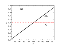
Seen from the relation between the proper time $\tau$ and the new time $s$ for the method $AS_{2}$ in Figure 1c, the proper time $\tau$ is about $9.7\times 10^{3}$ for the regular case of $\beta=0$, and about $8.1\times 10^{3}$ for the chaotic case of $\beta=9.7\times 10^{-4}$ when $s=10^{4}$. Namely, $\tau$ and $s$ are nearly consistent for the former case, and are somewhat different for the latter case.

Although the approximate equivalence of $\tau$ and $s$ is present in the method $AS_{2}$ for $\beta=0$, $AS_{2}$ still exhibits better accuracy in the integrals of motion than $S_{2}$. This is attributed to the application of the desired stretching and shrinking of the proper time steps $\Delta\tau$ to $AS_{2}$. $\Delta\tau$ grows nearly linearly with the distance $r$ in Figure 1d. Different step sizes appear in different values of $r$ during integration of the orbit. The step size is smaller for a shorter distance $r$, whereas larger for a longer distance $r$. This treatment of the step sizes is useful to significantly improve accuracy and efficiency of computations.

The accuracy of the method $AS_{2}$ relies on different choices of $j$ in Equation (22). The accuracy of integrations is improved typically as $j$ increases in Table 1. The difference between $\tau$ and $s$ gets larger, too. To make the difference as small as possible, we roughly take $j\sim(r_{min}+r_{max})/2$, where $r_{min}$ is the smallest distance of the bounded orbit. Based on better accuracy and extremely smaller difference between $\tau$ and $s$, $j=100$ is perhaps a better choice in the present situation.

We have demonstrated in detail an efficient implementation of the adaptive time step explicit symplectic integration algorithm to the Schwarzschild spacetime. The implementation is relatively easy because this spacetime has its Hamiltonian system that can be directly split into several explicitly integrable terms without time transformation (i.e. $g=1$). There are many other black hole spacetimes satisfying this property. In fact, the known spacetimes, including Reissner-Nordström black hole (Wang et al. 2021b), Reissner-Nordström-(anti)-de Sitter black hole (Wang et al. 2021c), modified gravity Schwarzschild black hole (Yang et al. 2022), rotating black ring (Wu et al. 2022), Brane-world metric (Hu $\&$ Huang 2022), Einstein-Æther black hole (Liu $\&$ Wu 2023), Konoplya-Zhidenko black hole (He et al. 2023), and Horndeski gravity hairy black hole (Cao et al. 2024), have been given the desired splitting forms. Without doubt, our adaptive time step explicit symplectic scheme should also be well suited for studies of these spacetimes.

The Kerr spacetime describes a rotating black hole geometry, which has covariant nonzero components (Kerr 1963):

	$\displaystyle g_{tt}=-(1-\frac{2r}{\Sigma}),~{}~{}g_{t\phi}=-\frac{2ar\sin^{2}\theta}{\Sigma}=g_{\phi t},$
	$\displaystyle g_{rr}=\frac{\Sigma}{\Delta},~{}~{}~{}~{}~{}~{}~{}~{}~{}~{}~{}~{}g_{\theta\theta}=\Sigma,$
	$\displaystyle g_{\phi\phi}=(\rho^{2}+\frac{2ra^{2}}{\Sigma}\sin^{2}\theta)\sin^{2}\theta,$		(36)

which $\Delta=\rho^{2}-2r$ and $\rho^{2}=r^{2}+a^{2}$. The dimensionless spin parameter $a$ corresponds to its practical spin $a_{pl}=aM$. For the Kerr geometry, the Hamiltonian (2) cannot be directly split into more than two explicitly integrable parts because $\Sigma$ acts as the denominators of the second, third terms of Equation (2). However, Wu et al. (2021) can still split the time-transformed Hamiltonian (6) into five explicit analytical solvable terms using the time transformation function $g$ of Equation (11) to eliminate the factor $\Sigma$ of the denominators. This brings a good chance for the application of the method $S_{2}$. Naturally, the method $AS_{2}$ is easily available, too.

Ernst (1976) gave a Schwarzschild-Melvin black hole describing the Schwarzschild black hole immersed in the magnetic universe of Melvin (1965). This black hole is an exact solution of Einstein’s equations. Besides the solution, the Reissner-Nordström-Melvin black hole and Kerr-Newman-Melvin black hole were presented. The Schwarzschild-Melvin black hole has nonzero metric components

	$\displaystyle g_{tt}=-\Lambda^{2}\left(1-\frac{2}{r}\right),~{}~{}g_{rr}=\Lambda^{2}\left(1-\frac{2}{r}\right)^{-1},$
	$\displaystyle g_{\theta\theta}=\Lambda^{2}r^{2},~{}~{}~{}~{}~{}~{}~{}~{}~{}~{}~{}~{}~{}~{}~{}~{}g_{\phi\phi}=\Lambda^{-2}r^{2}\sin^{2}\theta,$		(37)

where function $\Lambda$ is given by

$\displaystyle\Lambda=1+\frac{1}{4}B^{2}r^{2}\sin^{2}\theta.$

(38)

The dimensionless magnetic field $B$ corresponds to the practical one $B_{pl}=B/M$.

If the magnetic field vanishes, this spacetime is the Schwarzschild black hole. When it is nonzero, it acts as a gravitational effect, which causes this spacetime not to be asymptotically flat. If $|B|\ll 1$ and $2\ll r\ll 1/B$, then $\Lambda\approx 1$ outside the horizon. This means the existence of the approximately flat spacetime and the approximately uniform magnetic field. In this case, this spacetime is nearly integrable. This fact was confirmed by finding chaos of neutral particles around the Schwarzschild-Melvin black hole in the works of Karas $\&$ Vokrouhlický (1992) and Li $\&$ Wu (2019). Of course, neutral particles can also be chaotic in the Reissner-Nordström-Melvin black hole spacetime (Yang et al. 2023) and Kerr-Newman-Melvin black hole spacetime (Yang $\&$ Wu 2023). On the other hand, self-similar fractal structures appear in the shadows of the Schwarzschild-Melvin black hole (Junior et al. 2021) and Kerr-Melvin black hole (Wang et al. 2021; Hou et al. 2022). The chaotic lensing, i.e. the chaotic motion of photons, is responsible for these self-similar fractal structures in the black hole shadows.

We select the time transformation function of Equation (5) as

$\displaystyle g=\Lambda^{2}.$

(39)

The time-transformed Hamiltonian $K$ of Equation (6) resembles the Hamiltonian $H$ of Schwarzschild black hole in Equation (30) with $\beta=0$. That is, it consists of four explicitly integrable terms. In fact, only Equation (32) in Equations (32)-(35) is slightly modified as

$\displaystyle K_{1}=-\frac{rE^{2}}{2(r-2)}+\frac{L^{2}\Lambda^{4}}{2r^{2}\sin^{2}\theta}+p_{0}\Lambda^{2}.$

(40)

Although $E$ and $L$ are usually called as the energy and angular momentum of the photon in the Schwarzschild-Melvin spacetime, they are unlike those in the Kerr metric. For the former spacetime, $E$ is not the particle’s or photon’s energy measured by an observer at spatial infinity unless the observer lies on the axis of symmetry (Junior et al. 2021). However, $E$ is always the energy measured at spatial infinity for the latter spacetime. It is clear that the methods $AS_{2}$ and $S_{2}$ are suitably applicable to the time-transformed Hamiltonian $K$ of the Schwarzschild-Melvin black hole spacetime.

References

- Bacchini et al. (2018) Bacchini, F., Ripperda, B., Chen, A. Y., Sironi, L. 2018, ApJS, 237, 6
- Bacchini et al. (2019) Bacchini, F., Ripperda, B., Chen, A. Y., Sironi, L. 2019, ApJS, 240, 40
- Bardeen & Cunningham (1973) Bardeen, C. T., Cunningham, J. M. 1973, ApJ, 183, 237
- Blanes et al. (2024) Blanes, S., Casas, F., Escorihuela-Tomàs, A. 2024, Appl. Numer. Math. 204, 86
- Blanes et al. (2008) Blanes, S., Casas, F., Murua, A. 2008, Bol. Soc. Esp. Math. Apl., 45, 89
- Blanes et al. (2010) Blanes, S., Casas, F., Murua, A. 2010, Bol. Soc. Esp. Math. Apl., 50, 47
- Blanes & Moan (2002) Blanes, S., Moan, P. C. 2002, JCoAM, 142, 313
- Brown (2006) Brown, J. D. 2006, PhRvD, 73, 024001
- Cao et al. (2024) Cao, W., Wu, X., Lyv, J. 2024, Eur. Phys. J. C, 84, 435
- Cisterna & Erices (2014) Cisterna, A., Erices, C. 2014, PhRvD, 89, 084038
- Contreras et al. (2021) Contreras, E., Ovalle, J., Casadio, R. 2021, PhRvD, 103, 044020
- Cunha et al. (2015) Cunha, P. V. P., Herdeiro, C. A. R., Radu, E., Rúnarsson, H. F. 2015, PhRvL, 115, 211102
- Cunha et al. (2016) Cunha, P. V. P., Herdeiro, C. A. R., Radu, E., Rúnarsson, H. F., Wittig, A. 2016, PhRvD, 94, 104023
- Dolan & Shipley (2016) Dolan, S. R., Shipley, J. O. 2016, PhRvD, 94, 044038
- EHT et al. (2019) EHT Collaboration, et al. 2019, ApJL, 875, L1
- Emelýanenko (2007) Emel’yanenko, V. V. 2007, Celest. Mech. Dyn. Astron., 98, 191
- Ernst (1976) Ernst, F. J. 1976, J. Math. Phys., 17, 54
- Feng (1986) Feng, K. 1986, JCM, 44, 279
- Gao & Deng (2021) Gao, B., Deng, X. M. 2021, Eur. Phys. J. C, 81, 983
- García et al. (1995) García, A., Galtsov, D., Kechkin, O. 1995, PhRvL, 74, 1276
- He et al. (2023) He, G., Huang, G., Hu, A. 2023, Symmetry, 15, 1848
- Hou et al. (2022) Hou, Y., Zhang, Z., Yan, H., Guo, M., Chen, B.2022, PhRvD, 106, 064058
- Hu & Huang (2022) Hu, A., Huang, G.. 2022,Universe, 8, 369
- Hu & Huang (2023) Hu, A., Huang, G. 2023,Symmetry, 15, 1094
- Huang & Deng (2024) Huang, L., Deng, X. M. 2024, PhRvD,109, 124005
- Huang et al. (2022) Huang, Z., Huang, G., Hu, A.2022, ApJ, 925, 158
- Islam et al. (2023) Islam, S. U., Kumar, J., Walia, R. K., Ghosh, S. G. 2023, ApJ, 943, 22
- Jayawardana & Ohsawa (2023) Jayawardana, B., Ohsawa, T. 2023, Mathematics of Computation, 92, 251
- Johannsen (2013) Johannsen, T. 2013, ApJ, 777, 170
- Junior et al. (2021) Junior, H. C. D. L., Cunha, P. V. P., Herdeiro, C. A. R., Crispino, L. C. B. 2021, PhRvD, 104, 044018
- Karas & Vokrouhlický (1992) Karas, V., Vokrouhlický, D. 1992, General Relativity and Gravitation, 24, 729
- Kawashima et al. (2023) Kawashima, T., Ohsuga, K., Takahashi, H. R. 2023, ApJ, 949, 101
- Kerr (1963) Kerr, R. P. 1963, PhRvL, 11, 237
- Kopáček & Karas (2018) Kopáček, O., Karas, V. 2018, ApJ, 853, 53
- Kopáček et al. (2010) Kopáček, O., Karas, V., Kovár, J., Stuchlík, Z. 2010, ApJ, 722, 1240
- Kološ et al. (2021) Kološ, M., Tursunov, A., Stuchlík, Z. 2021, PhRvD, 103, 024021
- Kumar et al. (2022) Kumar, J., Islam, S. U., Ghosh, S. 2022, JCAP, 2022, 032
- Li & Wu (2019) Li, D., Wu, X. 2019, European Physical Journal Plus, 134, 96
- Liu & Wu (2023) Liu, C., Wu, X. 2023, Universe, 9, 365
- Lu & Wu (2024) Lu, J., Wu, X. 2024, Universe, 10, 277
- Melvin (1965) Melvin, M. A. 1965, Phys. Rev. B, 139, 225
- Mikkola (1997) Mikkola, S. 1997, Celest. Mech. Dyn. Ast., 67, 145
- Mikkola & Tanikawa (1999) Mikkola, S., Tanikawa, K. 1999, Celest. Mech. Dyn. Ast., 74, 287
- Mikkola & Tanikawa (2013) Mikkola, S., Tanikawa, K. 2013, New Astronomy, 20, 38
- Ohsawa (2023) Ohsawa, T. 2023, SIAM Journal on Numerical Analysis, 61 (3), 1293
- Pánis et al. (2019) Pánis, R., Kološ, M., Stuchlík, Z. 2019, Eur. Phys. J. C, 79, 479
- Pelle et al. (2022) Pelle, J., Reula, O., Carrasco, F., Bederian, C. 2022, MNRAS, 515, 1316
- Pihajoki (2015) Pihajoki, P. 2015, Celestial Mech. Dynam. Astronom., 121, 211
- Preto & Saha (2009) Preto, M., Saha, P. 2009, ApJ, 703, 1743
- Preto & Tremaine (1999) Preto, M., Tremaine, S. 1999, AJ, 118, 2532
- Pu et al. (2022) Pu, H., Yun, K., Younsi, Z., Yoon, S. 2016, ApJ, 820, 105
- Ruth (1983) Ruth, R. D. 1983, ITNS, 30, 2669
- Seyrich & Lukes-Gerakopoulos (2012) Seyrich, J., Lukes-Gerakopoulos, G. 2012, PhRvD, 86, 124013
- Pu et al. (2022) Stuchlík, Z., M. Kološ, M. 2016, Eur. Phys. J. C, 76, 32
- Pu et al. (2022) Sun, W., Wang, Y., Liu, F., Wu, X. 2021a, Eur. Phys. J. C, 81, 785
- Pu et al. (2022) Sun, X., Wu, X., Wang, Y., Deng, C., Liu, B., Liang, E. 2021b, Universe, 7, 410
- Seyrich & Lukes-Gerakopoulos (2012) Takahashi, M., Koyama, H. 2009, ApJ, 693, 472
- Pu et al. (2022) Tsang, D., Galley, C. R., Stein, L. C., Turner, A. 2015, ApJL, 809, L9
- Pu et al. (2022) Tursunov, A., Stuchlík, Z., Kološ, M. 2016, PhRvD, 93, 084012
- Pu et al. (2022) Tursunov, A., Stuchlík, Z., Kološ, M., Dadhich, N., Ahmedov, B. 2020, ApJ, 895, 14
- Ruth (1983) Virbhadra, K. S. 2024, PhRvD, 109, 124004
- Pu et al. (2022) Virbhadra1, K. S., Narasimha, D., Chitre, S. M. 1998, Astron. Astrophys., 337, 1
- Ruth (1983) Wald, R. M. 1974, PhRvD, 10, 1680
- Pu et al. (2022) Wang, M., Chen, S., Jing, J. 2021d, PhRvD, 104, 084021
- Pu et al. (2022) Wang Y., Sun W., Liu F., Wu X. 2021a, ApJ, 907, 66
- Pu et al. (2022) Wang Y., Sun W., Liu F., Wu X., 2021b, ApJ, 909, 22
- Pu et al. (2022) Wang Y., Sun W., Liu F., Wu, X. 2021c, ApJS, 254, 8
- Ruth (1983) White, C. J. 2022, ApJS, 262, 28
- Ruth (1983) Wisdom, J. 1982, AJ, 87, 577
- Seyrich & Lukes (2012) Wisdom, J., Holman, M. 1991, AJ, 102, 1528
- Pu et al. (2022) Wu, X., Wang, Y., Sun, W., Liu, F. Y. 2021, ApJ, 914, 63
- Pu et al. (2022) Wu, X., Wang, Y., Sun, W., Liu, F. Y, Han, W. B. 2022, ApJ, 940, 166
- Pu et al. (2022) Yang, D., Cao, W., Zhou, N., Zhang, H., Liu, W., Wu, X. 2022, Universe, 8, 320
- Pu et al. (2022) Yang, D., Liu, W., Wu, X. 2023, Eur. Phys. J. C, 83, 357
- Pu et al. (2022) Yang, D., Wu, X. 2023, Eur. Phys. J. C, 83, 789
- Ruth (1983) Yoshida, H. 1990, Phys. Lett. A, 150, 262
- Pu et al. (2022) Younsi, Z., Psaltis, D., Özel, F. 2023, ApJ, 942, 47
- Seyrich & Lukes (2012) Zhang, J., Xie, Y. 2022, Eur. Phys. J. C, 82, 854
- Pu et al. (2022) Zhang, H., Zhou, N., Liu, W., Wu, X. 2021, Universe, 7, 488
- Pu et al. (2022) Zhang, H., Zhou, N., Liu, W., Wu, X. 2022, General Relativity and Gravitation, 54, 110
- Pu et al. (2022) Zhou, N., Zhang, H., Liu, W., Wu, X. 2022, ApJ, 927, 160; 2023, ApJ, 947, 94