Explicit regularization and implicit bias in deep network classifiers trained with the square loss
Abstract
Deep ReLU networks trained with the square loss have been observed to perform well in classification tasks. We provide here a theoretical justification based on analysis of the associated gradient flow. We show that convergence to a solution with the absolute minimum norm is expected when normalization techniques such as Batch Normalization (BN) or Weight Normalization (WN) are used together with Weight Decay (WD). The main property of the minimizers that bounds their expected error is the norm: we prove that among all the close-to-interpolating solutions, the ones associated with smaller Frobenius norms of the unnormalized weight matrices have better margin and better bounds on the expected classification error. With BN but in the absence of WD, the dynamical system is singular. Implicit dynamical regularization – that is zero-initial conditions biasing the dynamics towards high margin solutions – is also possible in the no-BN and no-WD case. The theory yields several predictions, including the role of BN and weight decay, aspects of Papyan, Han and Donoho’s Neural Collapse and the constraints induced by BN on the network weights.
1 Introduction
In the case of exponential-type loss functions a mechanism of complexity control underlying generalization was identified in the asymptotic margin maximization effect of minimizing exponential-type loss functions [1, 2, 3]. However, this mechanism
-
•
cannot explain the good empirical results that have been recently demostrated using the square loss[4];
-
•
cannot explain the empirical evidence that convergence for cross-entropy loss minimization depends on initialization.
This puzzle motivates our focus in this paper on the square loss. More details and sketches of the proofs can be found in [5].
Here we assume commonly used GD-based normalization algorithms such such as BN[6] (or WN[7]) together with weight decay (WD), since they appear to be essential for reliably[8] training deep networks (and were used by [4]. We also consider, however, the case in which neither BN nor WD are used111This was the main concern of the first version of [5]. showing that a dynamic “implicit regularization” effect for classification is still possible with convergence strongly depending on initial conditions.
1.1 Notation
We define a deep network with layers with the usual coordinate-wise scalar activation functions as the set of functions , where the input is , the weights are given by the matrices , one per layer, with matching dimensions. We sometime use the symbol as a shorthand for the set of matrices . There are no bias terms: the bias is instantiated in the input layer by one of the input dimensions being a constant. The activation nonlinearity is a ReLU, given by . Furthermore,
-
•
we define with defined as the product of the Frobenius norms of the weight matrices of the layers of the network and as the corresponding network with normalized weight matrices (because the ReLU is homogeneous [3]);
-
•
in the following we use the notation meaning , that is the ouput of the normalized network for the input ;
-
•
we assume ;
-
•
separability is defined as correct classification for all training data, that is . We call average separability when .
1.2 Regression and classification
In our analysis of the square loss, we need to explain when and why regression works well for classification, since the training minimizes square loss but we are interested in good performance in classification (for simplicity we consider here binary classification). Unlike the case of linear networks we expect several global zero square loss minima corresponding to interpolating solutions (in general degenerate, see [9] and reference therein). Although all interpolating solutions are optimal solutions of the regression problem, they will in general have different margins and thus different expected classification performance. In other words, zero square loss does not imply by itself neither large margin nor good expected classification. Notice that if is a zero loss solution of the regression problem, then . This is equivalent to where is the margin for . Thus the norm of a minimizer is inversely related to its average margin. In fact, for an exact zero loss solution of the regression problem, the margin is the same for all training data and it is equal to . Starting from small initialization, GD will explore critical points with growing from zero, as we will show. Thus interpolating solutions with small norm (corresponding to the best margin) may be found before large solutions which have worse margin. If the weight decay parameter is non-zero and large enough, there is independence from initial conditions. Otherwise, a near-zero initialization is required, as in the case of linear networks, though the reason is quite different and is due to an implicit bias in the dynamics of GD.
2 Dynamics and Generalization
Our key assumption is that the main property of batch normalization (BN) and weight normalization (WN) – the normalization of the weight matrices – can be captured by the gradient flow on a loss function modified by adding Lagrange multipliers.
Gradient descent on a modified square loss
| (1) |
with is in fact exactly equivalent to “Weight Normalization”, as proved in [3], for deep networks.
This dynamics can be written as and with . This shows that if then as mentioned in [8]. The condition yields, as shown in [5], . Here we assume that the BN module is used in all layers apart the last one, that is we assume and where is the number of layers222It is important to observe here that batch normalization – unlike Weight Normalization – leads not only to normalization of the weight matrices but also to normalization of each row of the weight matrices [3] because it normalizes separately the activity of each unit and thus – indirectly – the for each separately. This implies that each row in is normalized independently and thus the whole matrix is normalized (assuming the normalization of each row is the same for all rows). The equations in the main text involving can be read in this way, that is restricted to each row..
As we will show, the dynamical system associated with the gradient flow of the Lagrangian Equation 1 is “singular”, in the sense that normalization is not guaranteed at the critical points. Regularization is needed, and in fact it is common to use in gradient descent not only batch normalization but also weight decay. Weight decay consists of a regularization term added to the Lagrangian yielding
| (2) |
The associate gradient flow is then the following dynamical system
| (3) |
| (4) |
where the critical points are singulat for but are not singular for any arbitrarily small 333For the zero loss critical point is pathological, since even when implying that an un-normalized interpolating solution satisfies the equilibrium equations. Numerical simulations show that even for linear degenerate networks convergence is independent of initial conditions only if .. In particular, normalization is then effective at unlike in the case. As a side remark, SGD, as opposed to gradient flow, may help (especially with label noise) to counter to some extent the singularity of the case, even without weight decay, because of the associated random fluctuations around the pathological critical point.
The equilibrium value at is
| (5) |
Observe that if is smaller than and if average separability holds. Recall also that zero loss “global” minima (in fact arbitrarily close to zero for small but positive ) are expected to exist and be degenerate [9].
If we assume that the loss (with the constraint ) is a continuous function of the , then there will be at least one minimum of at any fixed , because the domain is compact. This means that for each there is at least a critical point of the gradient flow of , implying that for each critical for which , there is at least one critical point of the dynamical system in and .
Around we have
| (6) |
where the terms will be generically different from zero if .
The conclusions of this analysis can be summarized in
Observation 1
Assuming average separability, and gradient flow starting from small norm norm >0, grows monotonically until a minimum is reached at which This dynamics is expected even in the limit of , which corresponds to exact interpolation of all the training data at a singular critical point.
and
Observation 2
Minimizers with small correspond to large average margin . In particular, suppose that the gradient flow converges to a and which correspond to zero square loss. Among all such minimizers the one with the smallest (typically found first during the GD dynamics when increases from ), corresponds to the (absolute) minimum norm – and maximum margin – solutions.
In general, there may be several critical points of the for the same and they are typically degenerate (see references in [10]) with dimensionality , where is the number of weights in the network may be degenerate. All of them will correspond to the same norm and all will have the same margin for all of the training points.
Since usually the maximum output of a multilayer network is , the first critical point for increasing will be when becomes large enough to allow the following equation to have solutions
| (7) |
If gradient flow starts from very small and there is average separability, increases monotonically until such a minimum is found. If is large, then and will decrease until a minimum is found.
For large and very small , we expect many solutions under GD444It is interesting to recall [9] that for SGD – unlike GD – the algorithm will stop only when , which is the global minimum and corresponds to perfect interpolation. For the other critical points for which GD will stop, SGD will never stop but just fluctuate around the critical point.. The emerging picture is a landscape in which there are no zero-loss minima for . With increasing from there will be zero square-loss degenerate minima with the minimizer representing an almost interpolating solution (for ). We expect, however, that depending on the value of , there is a bias towards minimum even for large initializations and certainly for small intializations.
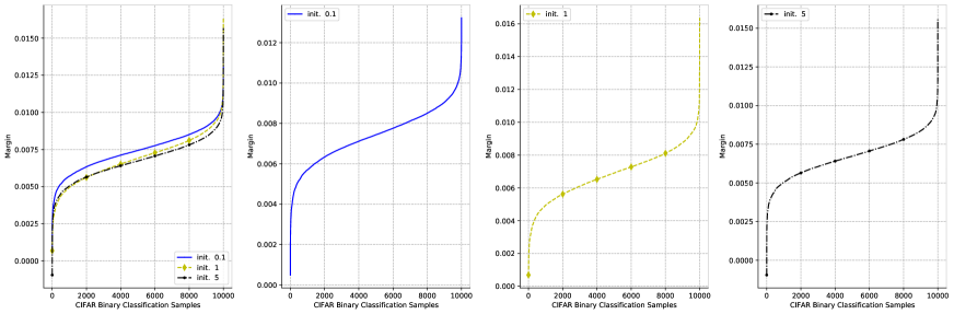
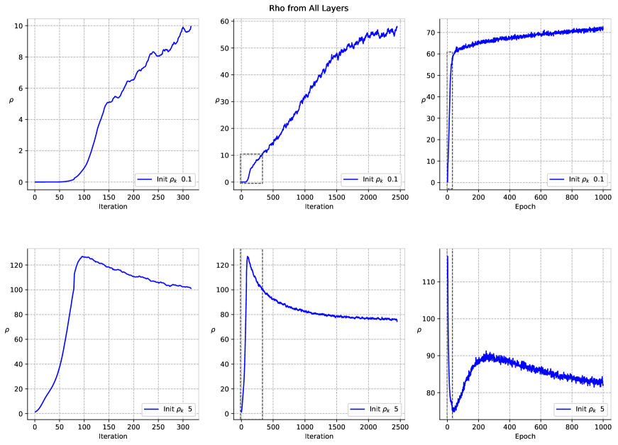
All these observations are also supported by our numerical experiments. Figure 1, 2, 3, and 4 show the case of gradient descent with batch normalization and weight decay, which corresponds to a well-posed dynamical system for gradient flow; the other figures show the same networks and data with BN without WD and without both BN and WD. As predicted by the analysis, the case of BN+WD is the most well-behaved, whereas the others strongly depend on initial conditions.


To show that indeed controls the expected error we use classical bounds that lead to the following theorem
Observation 3
With probability
| (8) |
where are constants that reflect the Lipschitz constant of the loss function ( for the square loss this requires a bound on ) and the architecture of the network. The Rademacher average depends on the normalized network architecture and . Thus for the same network and the same data, the upper bound for the expected error of the minimizer is smaller for smaller .
The theorem proves the conjecture in [11] that for deep networks, as for kernel machines, minimum norm interpolating solutions are the most stable.


2.1 Predictions
-
•
In a recent paper Papyan, Han and Donoho[12] described four empirical properties of the terminal phase of training (TPT) deep networks, using the cross-entropy loss function. TPT begins at the epoch where training error first vanishes. During TPT, the training error stays effectively zero, while training loss is pushed toward zero. Direct empirical measurements expose an inductive bias they call neural collapse (NC), involving four interconnected phenomena. (NC1) Cross-example within-class variability of last-layer training activations collapses to zero, as the individual activations themselves collapse to their class means. (NC2) The class means collapse to the vertices of a simplex equiangular tight frame (ETF). (NC3) Up to rescaling, the last-layer classifiers collapse to the class means or in other words, to the simplex ETF (i.e., to a self-dual configuration). (NC4) For a given activation, the classifier’s decision collapses to simply choosing whichever class has the closest train class mean (i.e., the nearest class center [NCC] decision rule). We show in [5] that these properties of the Neural Collapse[12] seem to be predicted by the theory of this paper for the global (that is, close-to-zero square-loss) minima, irrespectively of the value of . We recall that the basic assumptions of the analysis are Batch Normalization and Weight Decay. Our predictions are for the square loss but we show that they should hold also in the case of crossnetropy, explored in [12].
-
•
At a close to zero loss critical point of the flow, with in the training set, which are powerful constraints on the weight matrices to which training converges. A specific dependence of the matrix at each layer on matrices at the other layers is thus required. In particular, there are specific relations for each layer matrix of the type, explained in the Appendix,
(9) where the matrices are diagonal with components either or , depending on whether the corresponding ReLU unit is on or off.
As described in [5] for linear networks, a class of possible solutions to these constraint equations are projection matrices; another one are orthogonal matrices and more generally orthogonal Stiefel matrices on the sphere. These are sufficient but not necessary conditions to satisfy the constraint equations. Interestingly, randomly initialized weight matrices (an extreme case of the NTK regime) are approximately orthogonal.
3 Explicit Regularization and Implicit Dynamic Bias
We have established here convergence of the gradient flow to a minimum norm solution for the square loss, when gradient descent is used with BN (or WN) and WD. This result assumes explicit regularization (WD) and is thus consistent with [13], where is is proved that implicit regularization with the square loss cannot be characterized by any explicit function of the model parameters. We also show, however, that in the absence of WD and BN good solutions for binary classification can be found because of the bias in the dynamics of GD toward small norm solution introduced by near-zero initial conditions. Again, this is consistent with [13], because we identify an implicit bias in the dynamics which is relevant for classification.
For the exponential loss, BN is strictly not needed since minimization of the exponential loss maximizes the margin and minimizes the norm without BN, independently of initial conditions. Thus under the exponential loss, we expect a margin maximization bias for as shown in [14], independently of initial conditions. The effect however can require very long times and unreasonably high precision to have significant effect in practice.
If there exist several almost-interpolating solutions with the same norm , they also have the same margin for each of the training data. Though they have the same norm and the same margin on each of the data point, they may in principle have different ranks of the weight matrices or of the rank of the local Jacobian (at the minimum ) . Notice that in deep linear networks the GD dynamics biases the solution towards small rank solutions, since large eigenvalues converge much faster the small ones [15]. It in unclear whether the rank has a role in our analysis of generalization and we conjecture it does not.
Why does GD have difficulties in converging in the absence of BN+WD, especially for very deep networks? For square loss, the best answer is that good tuning of the learning rate is important and BN together with weight decay was shown to provide a remarkable autotuning [8]. A related answer is that regularization is needed to provide stability, including numerical stability.
4 Summary
The main results of the paper analysis can be summarized in the following
Lemma 1
If the gradient flow with normalization and weight decay converges to an interpolating solution with near-zero square loss, the following properties hold:
-
1.
The global minima in the square loss with the smallest are the global minimum norm solutions and have the best margin and the best bound on expected error;
-
2.
Conditions that favour convergence to such minimum norm solutions are batch normalization with weight decay () and small initialization (small );
-
3.
initialization with small can be sufficient to induce a bias in the dynamics of GD leading to large margin minimizers of the square loss;
-
4.
The condition which holds at the critical points of the SGD dynamics that are global minima, is key in predicting several properties of the Neural Collapse[12];
-
5.
the same condition represents a powerful constraint on the set of weight matrices at convergence.
4.1 Discussion
The role of the Lagrange multiplier term in Equation 1 is different from a standard regularization term because , determined by the constraint can be positive or negative, depending on the sign of the error . Thus the term acts as a regularizer when the norm of is larger than but has the opposite effect for , thus constraing each to the unit sphere. For the exponential loss, the situation is different and in acts as a positive regularization parameter, albeit a vanishing one (for ).
Are there any implications of the theory sketched here for mechanisms of learning in cortex? Somewhat intriguingly, some form of normalization, often described as a balance of excitation and inhibition, has long been thought to be a key function of intracortical circuits in cortical areas[16]. One of the first deep models of visual cortex models, HMAx, explored the biological plausibility of specific normalization circuits with spiking and non-spiking neurons. It is also interesting to note that the Oja rule describing synaptic plasticity in terms of changes to the synaptic weight is the Hebb rule plus a normalization term that corresponds to a Lagrange multiplier.
The main problems left open by this paper are:
-
•
The analysis is so far restricted to gradient flow. It should be exteded to gradient descent along the lines of [8].
-
•
It is remarkable that for the case of no BN and no WD, the dynamical system still yields good results, provided initialization is small. The case of BN+WD is the only one which seems rather independent of initial conditions in our experiments.
-
•
In this context, an extension of the analysis to SGD may also be critical for providing a satisfactory analysis of convergence.
Acknowledgments We are grateful to Shai Shalev-Schwartz, Andrzej Banbuski, Arturo Desza, Akshay Rangamani, Santosh Vempala, David Donoho, Vardan Papyan, X.Y. Han, Silvia Villa and especially to Eran Malach for very useful comments. This material is based upon work supported by the Center for Minds, Brains and Machines (CBMM), funded by NSF STC award CCF-1231216, and part by C-BRIC, one of six centers in JUMP, a Semiconductor Research Corporation (SRC) program sponsored by DARPA.
References
- [1] Mor Shpigel Nacson, Suriya Gunasekar, Jason D. Lee, Nathan Srebro, and Daniel Soudry. Lexicographic and Depth-Sensitive Margins in Homogeneous and Non-Homogeneous Deep Models. arXiv e-prints, page arXiv:1905.07325, May 2019.
- [2] Kaifeng Lyu and Jian Li. Gradient descent maximizes the margin of homogeneous neural networks. CoRR, abs/1906.05890, 2019.
- [3] A. Banburski, Q. Liao, B. Miranda, T. Poggio, L. Rosasco, B. Liang, and J. Hidary. Theory of deep learning III: Dynamics and generalization in deep networks. CBMM Memo No. 090, 2019.
- [4] Like Hui and Mikhail Belkin. Evaluation of neural architectures trained with square loss vs cross-entropy in classification tasks, 2020.
- [5] T. Poggio and Q. Liao. Generalization in deep network classifiers trained with the square loss. CBMM Memo No. 112, 2019.
- [6] Sergey Ioffe and Christian Szegedy. Batch normalization: Accelerating deep network training by reducing internal covariate shift. arXiv preprint arXiv:1502.03167, 2015.
- [7] Tim Salimans and Diederik P. Kingm. Weight normalization: A simple reparameterization to accelerate training of deep neural networks. Advances in Neural Information Processing Systems, 2016.
- [8] Sanjeev Arora, Zhiyuan Li, and Kaifeng Lyu. Theoretical analysis of auto rate-tuning by batch normalization. CoRR, abs/1812.03981, 2018.
- [9] T. Poggio and Y. Cooper. Loss landscape: Sgd has a better view. CBMM Memo 107, 2020.
- [10] T. Poggio and Y. Cooper. Loss landscape: Sgd can have a better view than gd. CBMM memo 107, 2020.
- [11] Tomaso Poggio. Stable foundations for learning. Center for Brains, Minds and Machines (CBMM) Memo No. 103, 2020.
- [12] Vardan Papyan, X. Y. Han, and David L. Donoho. Prevalence of neural collapse during the terminal phase of deep learning training. Proceedings of the National Academy of Sciences, 117(40):24652–24663, 2020.
- [13] Gal Vardi and O. Shamir. Implicit regularization in relu networks with the square loss. 2020.
- [14] Tomaso Poggio, Andrzej Banburski, and Qianli Liao. Theoretical issues in deep networks. PNAS, 2020.
- [15] Daniel Gissin, Shai Shalev-Shwartz, and Amit Daniely. The Implicit Bias of Depth: How Incremental Learning Drives Generalization. arXiv e-prints, page arXiv:1909.12051, September 2019.
- [16] RJ Douglas and KA Martin. Neuronal circuits of the neocortex. Annu Rev Neuroscience, 27:419–51, 2004.


