Explaining the differences in massive star models from various simulations
Abstract
The evolution of massive stars is the basis of several astrophysical investigations, from predicting gravitational-wave event rates to studying star-formation and stellar populations in clusters. However, uncertainties in massive star evolution present a significant challenge when accounting for these models’ behaviour in stellar population studies. In this work, we present a comparison between five published sets of stellar models from the BPASS, BoOST, Geneva, MIST and PARSEC simulations at near-solar metallicity. The different sets of stellar models have been computed using slightly different physical inputs in terms of mass-loss rates and internal mixing properties. Moreover, these models also employ various pragmatic methods to overcome the numerical difficulties that arise due to the presence of density inversions in the outer layers of stars more massive than 40 M⊙. These density inversions result from the combination of inefficient convection in the low-density envelopes of massive stars and the excess of radiative luminosity to the Eddington luminosity. We find that the ionizing radiation released by the stellar populations can change by up to 18 percent, the maximum radial expansion of a star can differ between 100–1600 R⊙, and the mass of the stellar remnant can vary up to 20 M⊙ between the five sets of simulations. We conclude that any attempts to explain observations that rely on the use of models of stars more massive than 40 M⊙ should be made with caution.
keywords:
stars: massive – stars: evolution – gravitational waves – stars: formation – stars: black holes – galaxies: stellar content1 Introduction
Stellar evolutionary model sequences serve as input for a broad range of astrophysical applications; from star-formation (e.g. Gatto et al., 2017) to galaxy evolution (e.g. Weinberger et al., 2020), from cluster dynamics (e.g. Heggie & Hut, 2003) to gravitational-wave studies (e.g. Vigna-Gómez et al., 2018). These sequences provide an easy and powerful way to account for both individual stars (e.g. Schneider et al., 2014) and stellar populations (e.g. Brott et al., 2011b) in a given astrophysical environment.
One dimensional (1D) model sequences (from now on: stellar models) can be computed from first principles (Kippenhahn & Weigert, 1990) and have become a household tool in astrophysical research. But when it comes to stars more massive than 9 M⊙ – those that, despite being rare, provide the bulk of the radiation, chemical pollution and the most exotic death throes in the Universe (Woosley et al., 2002) – stellar models are still riddled with large uncertainties.
High-mass stars are born less often than their low-mass counterparts (Salpeter, 1955) and have comparatively shorter lives (Crowther, 2012). Consequently, observational constraints on their evolution are more difficult to obtain. The situation is further complicated by many massive stars being observed to be fast rotators (Ramírez-Agudelo et al., 2013), which breaks down perfect symmetry, and to have a close-by companion star (Sana et al., 2012), breaking the assumption of perfect isolation. Even for isolated, non-rotating single stars, the physical conditions both inside (Heger et al., 2000) and around (Lamers & Cassinelli, 1999) the star are so peculiar and complex that developing appropriate numerical simulations becomes highly challenging. This is why the evolution of massive stars remains an actively studied field to this day.
Much progress has been made in the last few decades concerning massive stars and their evolution. Mass loss in the form of high-velocity winds from massive stars is being intensively studied and accounted for in the models (Smith, 2014; Sander & Vink, 2020). Observations of massive stars from the Large and Small Magellanic Clouds are being used to constrain the efficiency of interior mixing processes (Brott et al., 2011a; Schootemeijer et al., 2019). 1D stellar models have also been updated to account for the effects of rotation (Maeder, 2009; Costa et al., 2019) and magnetic fields (Heger et al., 2005; Maeder & Meynet, 2005; Takahashi & Langer, 2021) which can significantly change their evolutionary paths (Walder et al., 2012; Petit et al., 2017; Groh et al., 2020).
Despite the progress, there are still many open questions surrounding the lives of massive (9 M⊙) and ‘very’ massive (here designated as 40 M⊙) stars, and in the absence of well-defined answers, stellar evolution codes make use of different assumptions. Earlier studies comparing models of massive stars from different codes (e.g. Martins & Palacios, 2013; Jones et al., 2015) have already established that the differences in the physical parameters such as mixing and mass-loss rates adopted by various stellar evolution codes can affect the evolutionary outcome of these stars.
Here we highlight another major uncertainty arising due to the numerical treatment of low-density envelopes of very massive stars. These stars have luminosities close to the Eddington-limit, so changes in the elemental opacities during their evolution can lead to the formation of density and pressure inversions in the stellar envelope (Langer, 1997). The presence of these density inversions can cause numerical instabilities for 1D stellar evolution codes. To deal with these instabilities, the codes use different pragmatic solutions whose interplay with mixing and mass loss can further vary the evolution of massive stars.
The role of the Eddington limit and the associated density inversions in massive stars is well known within the stellar evolution community but remains relatively unknown outside the field. With the surge in the use of massive star models, for example, in gravitational-wave event rate predictions and supernova studies, it has become important to be aware of this issue. Our goal is to present the broader community with a concise overview, including how it affects the evolutionary properties such as the radial expansion and the remnant mass of very massive stars. To this end, we compare models of massive and very massive stars from five published sets created with different evolutionary codes: (i) models from the PAdova and TRieste Stellar Evolution Code (PARSEC; Bressan et al., 2012; Chen et al., 2015); (ii) the MESA Isochrones and Stellar Tracks (MIST; Choi et al., 2016) from the Modules for Experiments in Stellar Astrophysics (MESA; Paxton et al., 2011); (iii) models (Ekström et al., 2012; Yusof et al., 2013) from the Geneva code (Eggenberger et al., 2008); (iv) models from the Binary Population and Spectral Synthesis (BPASS; Eldridge et al., 2017) project; and (v) the Bonn Optimized Stellar Tracks (BoOST; Szécsi et al., 2022) from the ‘Bonn’ Code.
We describe the major physical ingredients used in computing each set of models in Section 2 and Section 3. In Section 4, we compare the predictions from each set of models in the Hertzsprung-Russell diagram and in terms of the emitted ionizing radiation, as well as the predictions for the maximum radial expansion of stars, and their remnant masses. Finally we draw conclusions in Section 5.
2 Physical inputs
| Stellar Model | Z⊙ | Hot Wind | Cool Wind | Wolf-Rayet Wind | Convective boundary | Overshoot type | |||
|---|---|---|---|---|---|---|---|---|---|
| BPASS | 0.020 | Vink et al. (2000, 2001) | de Jager et al. (1988) | Nugis & Lamers (2000) | Schwarzschild (1958) | 2.0 | Pols et al. (1998) | 0.12e | – |
| BOOST | 0.008a | Vink et al. (2000, 2001) | Nieuwenhuijzen & de Jager (1990) | Hamann et al. (1995)b | Ledoux (1947) | 1.5 | step | 0.335 | 1.0 |
| GENEVA | 0.014 | Vink et al. (2000, 2001) | de Jager et al. (1988)c | Nugis & Lamers (2000) | Schwarzschild (1958) | 1.6d | step | 0.1 | – |
| MIST | 0.014 | Vink et al. (2000, 2001) | de Jager et al. (1988) | Nugis & Lamers (2000) | Ledoux (1947) | 1.82 | Herwig (2000) | 0.016e | 0.1 |
| PARSEC | 0.015 | Vink et al. (2000, 2001) | de Jager et al. (1988) | Nugis & Lamers (2000) | Schwarzschild (1958) | 1.74 | Bressan et al. (1981) | 0.5e | – |
-
Notes.
-
a
For calculating mass-loss rates and opacities, Z⊙ is used.
-
b
Reduced by a factor of 10.
-
c
For , mass-loss rates from Crowther (2000) are used.
-
d
For stars with initial mass 40 M⊙, is used but with a different scale height (see Section 3).
-
e
The rough equivalent in the step overshooting formalism is 0.2, 0.25 and 0.4 for the MIST, PARSEC and BPASS models respectively.
2.1 Chemical composition
The chemical composition of the Sun is often used as a yardstick in computing the metal content of other stars. However, the exact value remains inconclusive and has undergone several revisions since 2004 (see Basu, 2009; Asplund et al., 2021, for an overview). Therefore, different stellar models often make use of different abundance scales.
The BPASS, PARSEC, Geneva and MIST models base their chemical compositions on the Sun, while the BoOST models use a mixture tailored to the sample of massive stars from the FLAMES survey (Evans et al., 2005) with . For stellar winds and opacity calculations, BoOST models use from Grevesse et al. (1996) as the reference solar metallicity. The BPASS models use solar abundances from Grevesse & Noels (1993) with Z⊙. The PARSEC models follow Grevesse & Sauval (1998) with revisions from Caffau et al. (2011) and Z⊙. Geneva models use Asplund et al. (2005) abundances with Ne abundance from Cunha et al. (2006) and Z⊙ while, finally, the MIST models base their abundance on Asplund et al. (2009) with Z⊙.
For the purpose of comparison here, we use models for each set except for BoOST where we use the Galactic composition, as the closest match. Iron is an important contributor to metallicity, as numerous iron transition lines dominate both opacity and mass-loss rates, therefore directly affecting the structure of massive stars (e.g., Puls et al., 2000). The stellar models compared here have similar iron content, with the normalised number density ( ranging from (for BoOST models) to (for MIST models).
2.2 Mass-loss rates
Stellar mass is a key determinant of a star’s life and evolutionary outcome. It can, however, change as stars lose their outer layers in the form of stellar winds, and through interactions with a binary companion. Consequently, mass loss can affect not only the structure and chemical composition of the star, but is also important in determining its final state (Renzo et al., 2017).
For massive stars, the effects of mass loss are even more pronounced. The mass loss experienced by hot massive stars (O type stars and Wolf–Rayet stars) is known to be line-driven (Lamers & Cassinelli, 1999) while that of cool massive stars (red supergiants, Levesque, 2017) is suggested to be dust-driven. Both types of mass loss are an intensively studied subject. However, the complexity of the problem of atomic and molecular transitions in the wind together with the rarity of stars at these high masses means that the model assumptions are usually based either on a few observations (a small sample of stars) or on what we know about the wind properties of low-mass stars.
All models in this study follow Vink et al. (2000, 2001) for hot wind-driven mass-loss. The PARSEC, Geneva, BPASS and MIST models follow de Jager et al. (1988) for cool dust-driven mass-loss and Nugis & Lamers (2000) for mass loss in the naked helium star phase. The Geneva models further switch to Crowther (2000) for hydrogen-rich stars with . They also use the maximum of Vink et al. (2001) and Gräfener & Hamann (2008) for stars with surface hydrogen mass fraction between 0.3 and 0.05, before switching to Nugis & Lamers (2000) when the surface hydrogen mass fraction falls below 0.05. The BoOST models follow Nieuwenhuijzen & de Jager (1990) for cool winds and Hamann et al. (1995, reduced by a factor of 10) for stars with surface hydrogen mass fraction . For computing mass-loss rates of stars with surface hydrogen mass fraction between 0.3 and 0.6, BoOST models linearly interpolate between the mass-loss rates of Vink et al. (2001) and Hamann et al. (1995, reduced by a factor of 10).
To account for the dependence of the mass-loss rates on the chemical composition, BoOST, MIST and BPASS models scale the mass-loss rates by a factor of (Vink et al., 2001) 111Note that for some models the factor is quoted, depending on whether the dependence of the terminal velocity on Z is explicitly considered or not.. Geneva and PARSEC models also use additional mass-loss as described in Section 3.
2.3 Convection and overshooting
Internal mixing processes such as convection and overshooting play an important role in determining both the structure and evolution of massive stars (e.g., see Sukhbold & Woosley, 2014). Similar to mass loss, these processes represent another major source of uncertainty in massive stellar evolution (Schootemeijer et al., 2019; Kaiser et al., 2020). In 1D stellar evolution codes convection is modelled using the Mixing-Length Theory (Böhm-Vitense, 1958, MLT) in terms of the mixing length parameter . However, 3D simulations suggest that convection in massive stars might be more sophisticated and turbulent than described by MLT (Jiang et al., 2015).
The BoOST, Geneva, PARSEC and BPASS models used here follow standard MLT (Cox & Giuli, 1968) for convective mixing with mixing length parameter = respectively. MIST follows a modified version of MLT given by Henyey et al. (1965) with . Convective boundaries in PARSEC, Geneva and BPASS models are determined using the Schwarzschild criterion (Schwarzschild, 1958). BoOST and MIST use the Ledoux criterion (Ledoux, 1947) for determining convective boundaries with semiconvective mixing parameters of 1.0 and 0.1, respectively. For determining convective core overshoot, Geneva and BoOST use step overshooting with overshoot parameter = . MIST uses exponential overshooting following Herwig (2000) with = 0.016. PARSEC uses overshoot from Bressan et al. (1981) with = . BPASS uses the overshoot prescription from Pols et al. (1998) with = 0.12. For comparison, the rough equivalent in the step overshooting formalism would be 0.2, 0.25 and 0.4 for the MIST, PARSEC and BPASS models respectively (See Choi et al., 2016; Pols et al., 1998; Bressan et al., 2012, for details of each method.)
MIST and PARSEC also include small amounts of overshoot associated with convective regions in the envelope. However, apart from modifying surface abundances, envelope overshoot has a negligible effect on the evolution of the star (Bressan et al., 2012). Rotational mixing also plays an important role in the evolution of massive stars. In fact, the calibration of the free parameters in the stellar codes is often based on their rotating models. For simplicity we only compare non-rotating models for PARSEC, MIST, Geneva and BPASS in this study. Although, for BoOST, in the absence of non-rotating models for stars more massive than 60 M⊙, we do use slowly rotating (100 km s-1) models. As shown by Brott et al. (2011a), this small difference in the initial rotation rate is not relevant from the point of view of the overall evolutionary behaviour.
Major input parameters used in each set of models are summarized in Table 1.
3 Eddington luminosity and the numerical treatment of density inversions
The Eddington luminosity is the maximum luminosity that can be transported by radiation while maintaining hydrostatic equilibrium (Eddington, 1926). In the low-density envelopes of massive stars changes in the elemental opacities during the evolution of stars can cause the local radiative luminosity to exceed the Eddington luminosity (Langer, 1997; Sanyal et al., 2015). To maintain hydrostatic equilibrium, density and pressure inversion regions form in the stellar envelope. In the absence of efficient convection (which is also typical for the low-density envelopes, Grassitelli et al. 2016), this can lead to convergence problems for 1D stellar evolution codes (Paxton et al., 2013). Owing to numerical difficulties, the time-steps become exceedingly small, preventing further evolution of the star. While less massive stars are only affected by this process in their late evolutionary phases (Harpaz, 1984; Lau et al., 2012), very massive stars can exceed the Eddington-limit already during the core-hydrogen-burning phase (Gräfener et al., 2012; Sanyal et al., 2015) and inhibit computation of their evolution. Therefore, 1D stellar evolution codes have to employ various solutions to compute further evolution of very massive stars.
In PARSEC models, density inversions and the consequent numerical difficulties are avoided by limiting the temperature gradient such that the density gradient never becomes negative (see Sec. 2.4 of Chen et al., 2015; Alongi et al., 1993). Limiting the temperature gradient prevents inefficient convection and the evolution of the stars proceeds uninterrupted. Also, the models include a mass-loss enhancement following Vink (2011) whenever the total luminosity of the star approaches the Eddington-luminosity.
MIST models suppress density inversions through the MLT++ formalism (Paxton et al., 2013) of MESA. In this method, the actual temperature gradient is artificially reduced to make it closer to the adiabatic temperature gradient whenever radiative luminosity exceeds the Eddington luminosity above a pre-defined threshold. This approach again increases convective efficiency, helping stars to overcome density inversions. Additionally, radiative pressure at the surface of the star is also enhanced in the MIST models to help with convergence (Choi et al., 2016).
In the extended envelopes of massive stars, the density scale height is much larger compared to the pressure scale height (which is typically used for computing the mixing length). Therefore, setting the mixing length to be comparable with the density scale height helps avoid density inversion (Nishida & Schindler, 1967; Maeder, 1987). The Geneva models include this treatment when computing models with initial masses greater than 40 M⊙ with (see Sec. 2.3 of Ekström et al., 2012). Additionally, the mass-loss rates for the models are increased by a factor of three whenever the local luminosity in any of the layers of the envelope is higher than five times the local Eddington luminosity.
BoOST models do not include any artificial treatment to prevent massive stars from encountering density inversions. Instead, their models undergo envelope inflation when massive stars reach the Eddington limit (Sanyal et al., 2015). On encountering the density inversions in their envelopes, the computation of very massive stars becomes numerically difficult. Further evolution of such stars is then computed through post-processing. It involves removing layers from the surface of the star (which would anyway happen due to regular mass loss) while correcting for surface properties such as effective temperature and luminosity (Szécsi et al., 2022).
BPASS models also allow density inversions to develop in the envelope of massive stars. However, these models are able to continue the evolution without numerical difficulties, most likely due to the use of a non-Lagrangian mesh (see Stancliffe, 2006, for an overview) and the resolution factors being lower than in other models (Eldridge et al., 2017; Eggleton, 1973).
4 Comparing the models
4.1 Differences between models in the Hertzsprung–Russell diagram
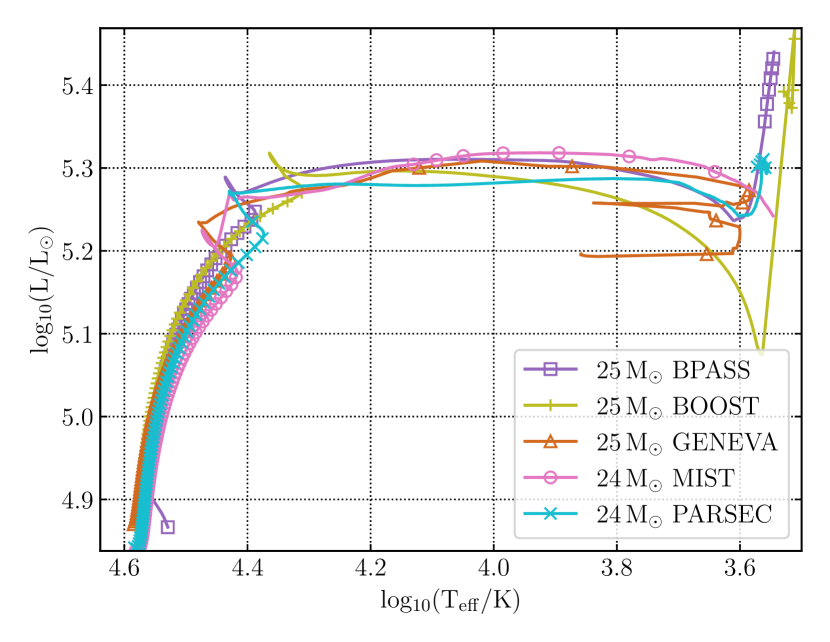
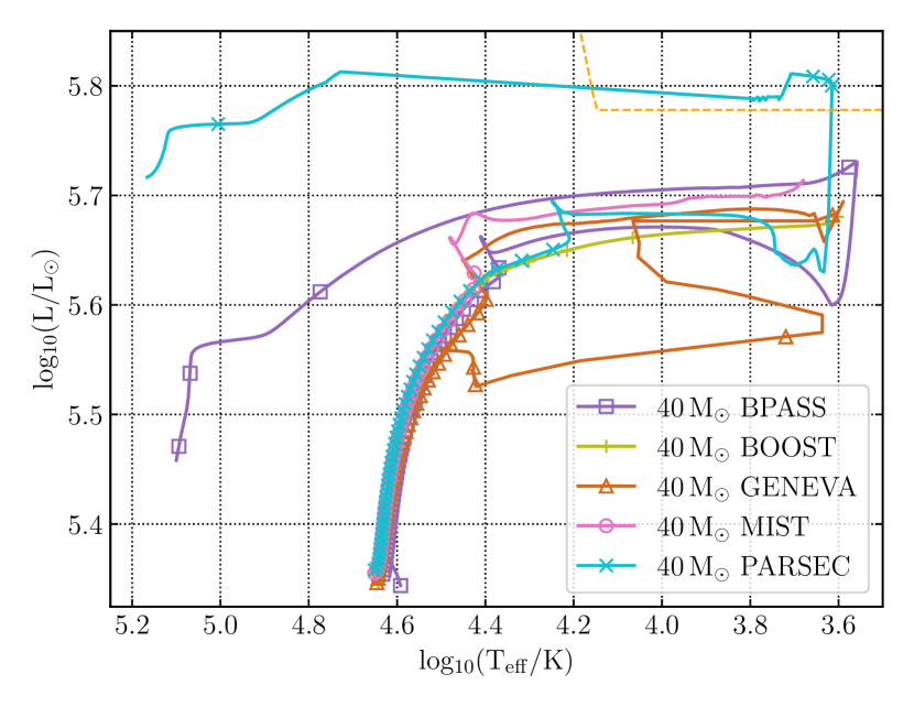
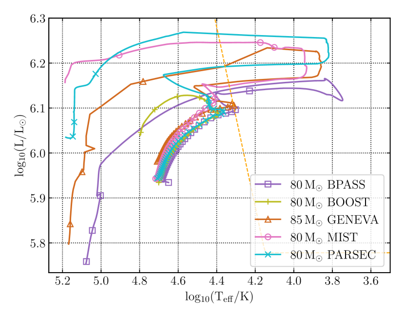
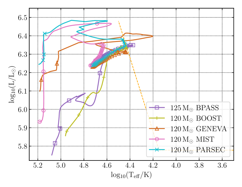
The evolution of stars can be easily represented through tracks on the Hertzsprung-Russell (HR) diagram, depicting the evolutionary paths followed by a series of stars. Figure 1 presents the HR diagram of stars of various initial masses from the five simulation approaches. The observational analogue to the Eddington-limit is the Humphreys–Davidson limit or HD-limit (Humphreys & Davidson, 1979). Since the luminosity of a star depends on its mass, more massive stars also are more luminous. This means they can easily exceed the Eddington-limit, develop density inversions and require the use of numerical solutions as discussed in Section 3.
From Figure 1 we see that the tracks of the 25 M⊙ (or 24 M⊙ in some cases) stars agree well during most of the evolution. This is because stars of this mass do not exceed the Eddington limit and are thus not affected by the related numerical treatments. The minor differences in their tracks are due to the difference in physical inputs (Section 2) between the simulations. For example, the differences in the position of the main-sequence (MS) hook feature in the HR diagram arise due to the varied extent of convective overshoot used in each set of models.
A 40 M⊙ star is clearly affected by the numerical treatment employed during the post-main sequence phase of its evolution, as evidenced by the difference in the tracks in the HR diagram shown in Figure 1. More massive stars, i.e, those with initial masses 80/85 M⊙ and 120/125 M⊙, can exceed the Eddington-limit in their envelopes while on the MS and therefore their simulations differ significantly from each other. At these masses, the mass-loss rates can be as high as 10-3 10-4 M⊙ yr-1, completely dominating over every other physical ingredient in determining the evolutionary path. While all tracks have been computed with similar prescriptions for wind mass loss (cf. Section 2), the actual rates can be strongly modified by the numerical methods adopted by each code in response to numerical instabilities (Section 3), resulting in vast differences in the tracks.
| Mini [M⊙] | 24/25 | 40 | 80/85 | 120/125 | pop. |
|---|---|---|---|---|---|
| PARSEC | |||||
| MIST | |||||
| Geneva | |||||
| BPASS | |||||
| BoOST |
4.2 Ionizing radiation and synthetic populations
The ionization released by a stellar population in e.g. a cluster or galaxy is influenced by the contribution of the most massive stars (Topping & Shull, 2015). As shown above however, these are the stars for which the simulations give the most diverse predictions.
To demonstrate this effect, we calculate the ionizing radiation emitted by a simple stellar population, supposing a Salpeter (1955) initial mass function with an upper mass of 120 M⊙ and a star-forming region of 107 M⊙ total mass – which is aimed to represent either a typical starburst galaxy, or a young massive cluster in the Milky Way. In Table 2 we list the Lyman photon flux predicted by the individual stellar models analysed here. To simplify the population synthesis calculations, the table provides time averaged values, that is, the photon number flux emitted over the whole evolution is divided by the lifetime. This way the emission coming from the population is estimated by simply weighting the time averaged values by the initial mass function (i.e. without needing to follow the time evolution of the modelled cluster or galaxy). The results of these simple population syntheses are also reported in Tab. 2. In the absence of spectral synthesis models computed for all five sets (cf. Wofford et al., 2016), we have opted to simply use black body estimation. To correct for optically thick winds, we follow the method explained in Chapter 4.5.1 of Szécsi (2016, which relies on ).
We find that, in terms of how much Lyman flux is emitted by a given synthetic population, the model predictions can differ as much as 18 percent between simulations. This supports earlier findings (e.g. Topping & Shull, 2015) that relying on the ionizing properties of massive stars from evolutionary models should be done with caution. Indeed one should keep in mind that the behaviour of the most massive models, those that dominate the radiation profile of any star-forming region, is weighted with large uncertainties – the source of which is the treatment of the Eddington limit, explained in Section 3.
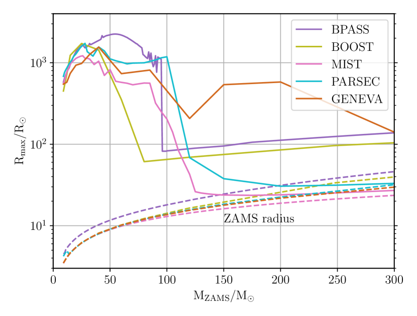
4.3 Predictions of maximum stellar radii
The radial expansion of a star plays a significant role in determining the nature of binary interaction as it can lead to episodes of mass transfer in close interacting binaries. Recent studies indicate that most of the massive stars occur in binaries (Sana et al., 2012; Moe & Di Stefano, 2017). Therefore, predictions of stellar radii become even more important for determining the binary properties of massive stars.
Figure 2 shows the maximum radial expansion achieved by massive stars from each simulation. For stars with initial mass up to 30 M⊙, all simulations predict the formation of a red supergiant. The maximum difference in the radius predictions here is 1000 R⊙. For higher initial masses, the predictions for maximum stellar radii become more divergent as proximity to the Eddington-limit increases and numerical treatments adopted by each code modify the mass-loss rates.
The greatest difference in the maximum radius predictions (1000 R⊙) occurs for stars with initial masses between 40 and 100 M⊙. Above 100 M⊙, stars have even higher mass-loss rates which can completely strip a star of its envelope before it can become a red-supergiant. Such stars evolve directly towards the naked helium star phase and have much smaller radii. Therefore, for stars with initial masses more than 100 M⊙, the difference between the maximum radius predictions by each simulation reduces to 100 R⊙. The predictions in this mass range seem to further converge into two main groups: PARSEC and MIST represent one group predicting smaller radii compared to the second group which consists of BoOST and BPASS models. The maximum radii in this mass range are predicted by the Geneva models. This is due to the difference in the mass loss rates adopted during the naked helium phase of the star, as explained in the next section.
4.4 Remnant mass predictions
 |

|

|
Stellar evolutionary models provide an easy way of estimating the properties of stellar remnants such as black holes and neutron stars, which are needed in many fields including supernova studies (e.g. Aguilera-Dena et al., 2018; Raithel et al., 2018), gamma-ray bursts progenitors (e.g. Yoon et al., 2006; Szecsi, 2017), and gravitational-wave event rate predictions (e.g. Stevenson et al., 2019; Mapelli et al., 2020).
Following Belczynski et al. (2010) we show in Figure 3 how the uncertainties in the models we compare here also pose a challenge for the predictions of remnant properties. Remnant masses have been calculated from the carbon-oxygen (CO) core mass and the total mass of the star at the end of the core helium-burning phase using the prescription of Belczynski et al. (2008) (same as the StarTrack prescription in Fryer et al., 2012).
The Geneva models do not provide information on core masses in their publicly available dataset. Therefore, the final CO-core mass for these models has been taken from Georgy et al. (2012, for stars with initial mass up to 120 M⊙) and Yusof et al. (2013, for stars with initial mass more than 120 M⊙). Note that in the Geneva models from Yusof et al. (2013), CO-core mass is defined as the mass of the core where the sum of mass fraction of carbon and oxygen exceeds 75 percent, and is different to the definition used by Georgy et al. (2012).
The remnant masses are heavily influenced by the modelling assumptions (cf. Section 2) and the numerical methods (cf. Section 3) especially above Mini 40 M⊙ where the most massive black holes are predicted. For stars with initial masses between 9 and 120 M⊙, we find that the mass of the black holes predicted by the different sets of models can differ by 20 M⊙. The maximum black hole mass varies from about 20 M⊙ for BPASS models to about 35 M⊙ for MIST and PARSEC models, and 32 M⊙ for the BoOST models. BPASS models consistently predict the lowest values of remnant mass for most of the massive stars while predictions from the BoOST, MIST and PARSEC models peak at 60, 90 and 120 M⊙ before flattening out at the higher initial masses.
For more massive stars, the variation in the remnant mass between BPASS, BoOST, MIST and PARSEC models reduces to about 10 M⊙. An interesting behaviour is shown by the Geneva models, which predict one of the lowest remnant masses for stars up to 120 M⊙, reaching a maximum of only 28 M⊙ at 120 M⊙. These models however, predict the highest values of remnant masses beyond 120 M⊙. At their farthest, for a model with initial mass of 200 M⊙, the predictions between the Geneva models and other models can be as high as 30 M⊙. Similar variability is found in the core mass and the final total mass of the star (from which the remnant masses have been calculated).
The significantly higher remnant masses predicted by the Geneva models for stars with initial mass beyond 120 M⊙can be explained as follows. Due to their high luminosity, stars more massive than 100–120 M⊙ rapidly lose mass during the main-sequence phase and directly evolve towards the naked helium phase (cf. Figure 1). The mass-loss prescriptions from both Nugis & Lamers (2000) and Hamann et al. (1995) predict the highest mass-loss rates for stars occur during this naked helium phase. BPASS, MIST and PARSEC models switch to mass-loss rates from Nugis & Lamers (2000) when the mass fraction of hydrogen at the surface of the star falls below 0.4, 0.4 and 0.5 respectively. BoOST models linearly interpolate between the mass-loss rates of Vink et al. (2001) and Hamann et al. (1995, reduced by a factor of 10) for stars with surface hydrogen mass fraction between 0.3 and 0.6, before completely switching to the mass-loss rate from Hamann et al. (1995, reduced by a factor of 10) for stars with surface hydrogen mass fraction less than 0.3.
Geneva models, on the other hand, switch to using mass-loss rates from Nugis & Lamers (2000) only when the mass fraction of hydrogen at the surface of the star falls below 0.05. For stars with surface hydrogen mass fraction between 0.3 and 0.05, they use the maximum of Vink et al. (2001) and Gräfener & Hamann (2008), which predict lower mass-loss rates compared to both Nugis & Lamers (2000) and Hamann et al. (1995) (See section 2.1 of Yusof et al., 2013). Thus, they do not lose as much mass as other models during the naked helium star phase and end with higher total mass and thus with the higher remnant mass.
Note that the Belczynski et al. (2008) prescription is one of several methods for predicting the remnant properties of the stars. Other methods for calculating the remnant masses may predict higher or lower values. For example, the remnant mass calculations based on the binding energy of the star (e.g. see Eldridge et al., 2017) are generally lower than those predicted here. However, all the models we study have near-solar metallicity and therefore rather high mass-loss rates, none of them stays massive enough at the end of their lives to undergo pair-instability.
5 Conclusions
We compare 1D evolutionary models of massive and very massive stars from five independent simulations. Focusing on near-solar composition, we find that the predictions from different codes can differ from each other by more than 1000 R⊙ in terms of maximum radial expansion achieved by the stars, by 18 percent in terms of ionizing radiation, and about 20 M⊙ in terms of the stellar remnant mass. The differences in the evolution of massive stars can arise due to physical inputs like chemical abundances, mass-loss rates, and internal mixing properties. However, very massive stars, that is stars with initial masses 40 M⊙ or more, show a larger difference in evolutionary properties compared to lower mass stars. For these stars, the differences in the evolution can be largely attributed to the numerical treatment of the models when the Eddington-limit is exceeded in their low-density envelopes.
The different methods used by 1D codes to compute the evolution of massive stars beyond density inversions (or to avoid the inversions) can modify the radius and temperature of the star, and can therefore affect the mass-loss rates. A phenomenological justification for the mass loss enhancement comes from the fact that there are stars observed with extremely high, episodical mass loss, i.e. luminous blue variables (Bestenlehner et al., 2014; Sarkisyan et al., 2020). However, other studies, such as the recent measurement of a approximately 20 M⊙ black hole in the Galactic black hole high-mass X-ray binary Cyg X-1 (Miller-Jones et al., 2021), suggest that the mass-loss rates for massive stars at near-solar metallicity may be lower than usually assumed in the 1D stellar models (Neijssel et al., 2021). The exact nature of wind mass loss for very massive stars remains disputed (Smith & Tombleson, 2015). Moreover, variation in remnants masses in Figure 3 shows other uncertainties in massive star evolution can lead to differences at least as large as variations in mass-loss rates, which could also easily explain the formation of a 20 M⊙ black hole in Cyg X-1 in the Galaxy.
None of the solutions that the BoOST, Geneva, MIST and PARSEC models employ can currently be established as better than the others. In each case they have been designed to address numerical issues in 1D stellar evolution. However, the interplay of these solutions with mass-loss rates and convection further adds to the uncertainties in massive stellar evolution. Therefore, a systematic study to untangle the effect of the treatment of the Eddington-limit from other physical assumptions has been conducted in a companion paper (Agrawal et al., 2021).
In the case of BPASS the stellar models evolve without requiring any numerical enhancement. Whether this is a result of using a non-Lagrangian mesh (the ‘Eggletonian’ mesh, which is more adaptive to changes in stellar structure) or if this is an artifact of bigger time steps (that helps stars skip problematic short-lived phases of evolution) is currently not known. A separate study to explore the effect of the ‘Lagrangian’ versus the ‘Eggletonian’ mesh structure for massive stars (similar to Stancliffe et al. 2004 study for low and intermediate mass stars) is highly desirable.
In conclusion, it is crucial to be aware of the uncertainties resulting from numerical methods whenever the evolutionary model sequences of massive stars are applied in any scientific project, such as gravitational-wave event rate predictions or star-formation and feedback studies.
We only focus on massive stars as isolated single stars in this work. However, there is mounting evidence that massive stars are formed as binaries or triples, thus treating them as single stars might not be correct (e.g., Klencki et al., 2020; Laplace et al., 2021). Several studies have shown that binarity can heavily influence the lives of massive stars through mass and angular momentum transfer (de Mink et al., 2009; Marchant et al., 2016; Eldridge et al., 2017) and can therefore help in avoiding density and pressure inversion regions in stellar envelopes (Shenar et al., 2020).
We also limit our study to massive stars at near-solar metallicity, where due to high opacity, the numerical instabilities related to the proximity to the Eddington-limit are maximum. Since opacity decreases with metallicity, opacity peaks become less prominent at lower metallicity. Nevertheless, stars with low-metal content also reach the Eddington-limit, although at higher initial masses (Sanyal et al., 2015, 2017). While progenitors of currently detectable gravitational-wave (GW) sources may have been born in the early Universe where the metal content is sub-solar (cf. Santoliquido et al., 2021), high star-formation rates at near solar metallicities offer a fertile ground for the formation of more GW sources, although less massive compared to sub-solar metallicity (Neijssel et al., 2019). As such, there is good motivation for studying the behaviour and reliability of massive star models across a wide range of metallicities (Agrawal et al., 2021).
Collecting observational data as well as improvements in 3D and hydrodynamical modelling will help us better constrain the models of massive stars in the future. Until then, however, we urge the broader community to treat any set of stellar models with caution. Ideally, one would implement all available simulations as input into any given astrophysical study, and test the outcome also in terms of stellar evolution related uncertainties. With tools such as METISSE (Agrawal et al., 2020) and SEVN (Spera et al., 2019), this task is becoming feasible.
Acknowledgements
DSz has been supported by the Alexander von Humboldt Foundation. PA, SS and JH acknowledges the support from the Australian Research Council Centre of Excellence for Gravitational Wave Discovery (OzGrav). We also thank Stefanie Walch-Gassner, Debashis Sanyal and Ross Church for useful comments and discussions. We are also grateful to the referee, Cyril Georgy for their suggestions which greatly improved the work.
Data Availability
All the stellar models used in this work are publicly available:
PARSEC: people.sissa.it/sbressan/parsec.html,
MIST: waps.cfa.harvard.edu/MIST/,
Geneva: obswww.unige.ch/Research/evol/tables_grids2011/Z014,
BPASS: bpass.auckland.ac.nz/9.html,
BoOST: boost.asu.cas.cz.
References
- Agrawal et al. (2020) Agrawal P., Hurley J., Stevenson S., Szécsi D., Flynn C., 2020, MNRAS, 497, 4549
- Agrawal et al. (2021) Agrawal P., Stevenson S., Szécsi D., Hurley J., 2021, arXiv e-prints, p. arXiv:2112.02801
- Aguilera-Dena et al. (2018) Aguilera-Dena D. R., Langer N., Moriya T. J., Schootemeijer A., 2018, ApJ, 858, 115
- Alongi et al. (1993) Alongi M., Bertelli G., Bressan A., Chiosi C., Fagotto F., Greggio L., Nasi E., 1993, A&AS, 97, 851
- Asplund et al. (2005) Asplund M., Grevesse N., Sauval A. J., 2005, in Barnes III T. G., Bash F. N., eds, Astronomical Society of the Pacific Conference Series Vol. 336, Cosmic Abundances as Records of Stellar Evolution and Nucleosynthesis. p. 25
- Asplund et al. (2009) Asplund M., Grevesse N., Sauval A. J., Scott P., 2009, ARA&A, 47, 481
- Asplund et al. (2021) Asplund M., Amarsi A. M., Grevesse N., 2021, A&A, 653, A141
- Basu (2009) Basu S., 2009, in Dikpati M., Arentoft T., González Hernández I., Lindsey C., Hill F., eds, Astronomical Society of the Pacific Conference Series Vol. 416, Solar-Stellar Dynamos as Revealed by Helio- and Asteroseismology: GONG 2008/SOHO 21. p. 193
- Belczynski et al. (2008) Belczynski K., Kalogera V., Rasio F. A., Taam R. E., Zezas A., Bulik T., Maccarone T. J., Ivanova N., 2008, ApJS, 174, 223
- Belczynski et al. (2010) Belczynski K., Bulik T., Fryer C. L., Ruiter A., Valsecchi F., Vink J. S., Hurley J. R., 2010, ApJ, 714, 1217
- Bestenlehner et al. (2014) Bestenlehner J. M., et al., 2014, A&A, 570, A38
- Böhm-Vitense (1958) Böhm-Vitense E., 1958, Z. Astrophys., 46, 108
- Bressan et al. (1981) Bressan A. G., Chiosi C., Bertelli G., 1981, A&A, 102, 25
- Bressan et al. (2012) Bressan A., Marigo P., Girardi L., Salasnich B., Dal Cero C., Rubele S., Nanni A., 2012, MNRAS, 427, 127
- Brott et al. (2011a) Brott I., et al., 2011a, A&A, 530, A115
- Brott et al. (2011b) Brott I., et al., 2011b, A&A, 530, A116
- Caffau et al. (2011) Caffau E., Ludwig H. G., Steffen M., Freytag B., Bonifacio P., 2011, Sol. Phys., 268, 255
- Chen et al. (2015) Chen Y., Bressan A., Girardi L., Marigo P., Kong X., Lanza A., 2015, MNRAS, 452, 1068
- Choi et al. (2016) Choi J., Dotter A., Conroy C., Cantiello M., Paxton B., Johnson B. D., 2016, ApJ, 823, 102
- Costa et al. (2019) Costa G., Girardi L., Bressan A., Marigo P., Rodrigues T. S., Chen Y., Lanza A., Goudfrooij P., 2019, MNRAS, 485, 4641
- Cox & Giuli (1968) Cox J., Giuli R., 1968, Principles of Stellar Structure: Physical principles. Principles of Stellar Structure, Gordon and Breach, https://books.google.com.au/books?id=TdhEAAAAIAAJ
- Crowther (2000) Crowther P. A., 2000, A&A, 356, 191
- Crowther (2012) Crowther P., 2012, Astronomy and Geophysics, 53, 4.30
- Cunha et al. (2006) Cunha K., Hubeny I., Lanz T., 2006, ApJ, 647, L143
- Eddington (1926) Eddington A. S., 1926, The Internal Constitution of the Stars. Cambridge Science Classics, Cambridge University Press, doi:10.1017/CBO9780511600005
- Eggenberger et al. (2008) Eggenberger P., Meynet G., Maeder A., Hirschi R., Charbonnel C., Talon S., Ekström S., 2008, Ap&SS, 316, 43
- Eggleton (1973) Eggleton P. P., 1973, MNRAS, 163, 279
- Ekström et al. (2012) Ekström S., et al., 2012, A&A, 537, A146
- Eldridge et al. (2017) Eldridge J. J., Stanway E. R., Xiao L., McClelland L. A. S., Taylor G., Ng M., Greis S. M. L., Bray J. C., 2017, Publications of the Astronomical Society of Australia, 34, e058
- Evans et al. (2005) Evans C. J., et al., 2005, A&A, 437, 467
- Fryer et al. (2012) Fryer C. L., Belczynski K., Wiktorowicz G., Dominik M., Kalogera V., Holz D. E., 2012, ApJ, 749, 91
- Gatto et al. (2017) Gatto A., et al., 2017, MNRAS, 466, 1903
- Georgy et al. (2012) Georgy C., Ekström S., Meynet G., Massey P., Levesque E. M., Hirschi R., Eggenberger P., Maeder A., 2012, A&A, 542, A29
- Gräfener & Hamann (2008) Gräfener G., Hamann W. R., 2008, A&A, 482, 945
- Gräfener et al. (2012) Gräfener G., Owocki S. P., Vink J. S., 2012, A&A, 538, A40
- Grassitelli et al. (2016) Grassitelli L., Fossati L., Langer N., Simón-Díaz S., Castro N., Sanyal D., 2016, A&A, 593, A14
- Grevesse & Noels (1993) Grevesse N., Noels A., 1993, in Prantzos N., Vangioni-Flam E., Casse M., eds, Origin and Evolution of the Elements. pp 15–25
- Grevesse & Sauval (1998) Grevesse N., Sauval A. J., 1998, Space Sci. Rev., 85, 161
- Grevesse et al. (1996) Grevesse N., Noels A., Sauval A. J., 1996, in Holt S. S., Sonneborn G., eds, Astronomical Society of the Pacific Conference Series Vol. 99, Cosmic Abundances. p. 117
- Groh et al. (2020) Groh J. H., Farrell E. J., Meynet G., Smith N., Murphy L., Allan A. P., Georgy C., Ekstroem S., 2020, ApJ, 900, 98
- Hamann et al. (1995) Hamann W. R., Koesterke L., Wessolowski U., 1995, A&A, 299, 151
- Harpaz (1984) Harpaz A., 1984, MNRAS, 210, 633
- Heger et al. (2000) Heger A., Langer N., Woosley S. E., 2000, ApJ, 528, 368
- Heger et al. (2005) Heger A., Woosley S. E., Spruit H. C., 2005, ApJ, 626, 350
- Heggie & Hut (2003) Heggie D., Hut P., 2003, The Gravitational Million-Body Problem: A Multidisciplinary Approach to Star Cluster Dynamics. Cambridge University Press
- Henyey et al. (1965) Henyey L., Vardya M. S., Bodenheimer P., 1965, ApJ, 142, 841
- Herwig (2000) Herwig F., 2000, A&A, 360, 952
- Humphreys & Davidson (1979) Humphreys R. M., Davidson K., 1979, ApJ, 232, 409
- Jiang et al. (2015) Jiang Y.-F., Cantiello M., Bildsten L., Quataert E., Blaes O., 2015, ApJ, 813, 74
- Jones et al. (2015) Jones S., Hirschi R., Pignatari M., Heger A., Georgy C., Nishimura N., Fryer C., Herwig F., 2015, MNRAS, 447, 3115
- Kaiser et al. (2020) Kaiser E. A., Hirschi R., Arnett W. D., Georgy C., Scott L. J. A., Cristini A., 2020, MNRAS, 496, 1967
- Kippenhahn & Weigert (1990) Kippenhahn R., Weigert A., 1990, Stellar Structure and Evolution. Springer
- Klencki et al. (2020) Klencki J., Nelemans G., Istrate A. G., Pols O., 2020, A&A, 638, A55
- Lamers & Cassinelli (1999) Lamers H., Cassinelli J., 1999, Introduction to Stellar Winds. Cambridge University Press
- Langer (1989) Langer N., 1989, A&A, 210, 93
- Langer (1997) Langer N., 1997, in Nota A., Lamers H., eds, Astronomical Society of the Pacific Conference Series Vol. 120, Luminous Blue Variables: Massive Stars in Transition. p. 83
- Laplace et al. (2021) Laplace E., Justham S., Renzo M., Götberg Y., Farmer R., Vartanyan D., de Mink S. E., 2021, arXiv e-prints, p. arXiv:2102.05036
- Lau et al. (2012) Lau H. H. B., Gil-Pons P., Doherty C., Lattanzio J., 2012, A&A, 542, A1
- Ledoux (1947) Ledoux P., 1947, ApJ, 105, 305
- Levesque (2017) Levesque E. M., 2017, Astrophysics of Red Supergiants. 2514-3433, IOP Publishing, doi:10.1088/978-0-7503-1329-2
- Maeder (1987) Maeder A., 1987, A&A, 173, 247
- Maeder (2009) Maeder A., 2009, Physics, Formation and Evolution of Rotating Stars. Springer Berlin Heidelberg, doi:10.1007/978-3-540-76949-1
- Maeder & Meynet (2005) Maeder A., Meynet G., 2005, A&A, 440, 1041
- Mapelli et al. (2020) Mapelli M., Spera M., Montanari E., Limongi M., Chieffi A., Giacobbo N., Bressan A., Bouffanais Y., 2020, ApJ, 888, 76
- Marchant et al. (2016) Marchant P., Langer N., Podsiadlowski P., Tauris T. M., Moriya T. J., 2016, A&A, 588, A50
- Martins & Palacios (2013) Martins F., Palacios A., 2013, A&A, 560, A16
- Miller-Jones et al. (2021) Miller-Jones J. C. A., et al., 2021, Science, 371, 1046
- Moe & Di Stefano (2017) Moe M., Di Stefano R., 2017, ApJS, 230, 15
- Neijssel et al. (2019) Neijssel C. J., et al., 2019, MNRAS, 490, 3740
- Neijssel et al. (2021) Neijssel C. J., Vinciguerra S., Vigna-Gómez A., Hirai R., Miller-Jones J. C. A., Bahramian A., Maccarone T. J., Mandel I., 2021, ApJ, 908, 118
- Nieuwenhuijzen & de Jager (1990) Nieuwenhuijzen H., de Jager C., 1990, A&A, 231, 134
- Nishida & Schindler (1967) Nishida M., Schindler A. M., 1967, PASJ, 19, 606
- Nugis & Lamers (2000) Nugis T., Lamers H. J. G. L. M., 2000, A&A, 360, 227
- Paxton et al. (2011) Paxton B., Bildsten L., Dotter A., Herwig F., Lesaffre P., Timmes F., 2011, ApJS, 192, 3
- Paxton et al. (2013) Paxton B., et al., 2013, ApJS, 208, 4
- Petit et al. (2017) Petit V., et al., 2017, MNRAS, 466, 1052
- Pols et al. (1998) Pols O. R., Schröder K.-P., Hurley J. R., Tout C. A., Eggleton P. P., 1998, MNRAS, 298, 525
- Puls et al. (2000) Puls J., Springmann U., Lennon M., 2000, A&AS, 141, 23
- Raithel et al. (2018) Raithel C. A., Sukhbold T., Özel F., 2018, ApJ, 856, 35
- Ramírez-Agudelo et al. (2013) Ramírez-Agudelo O. H., et al., 2013, A&A, 560, A29
- Renzo et al. (2017) Renzo M., Ott C. D., Shore S. N., de Mink S. E., 2017, A&A, 603, A118
- Salpeter (1955) Salpeter E. E., 1955, ApJ, 121, 161
- Sana et al. (2012) Sana H., et al., 2012, Science, 337, 444
- Sander & Vink (2020) Sander A. A. C., Vink J. S., 2020, MNRAS, 499, 873
- Santoliquido et al. (2021) Santoliquido F., Mapelli M., Giacobbo N., Bouffanais Y., Artale M. C., 2021, MNRAS, 502, 4877
- Sanyal et al. (2015) Sanyal D., Grassitelli L., Langer N., Bestenlehner J. M., 2015, A&A, 580, A20
- Sanyal et al. (2017) Sanyal D., Langer N., Szécsi D., -C Yoon S., Grassitelli L., 2017, A&A, 597, A71
- Sarkisyan et al. (2020) Sarkisyan A., et al., 2020, MNRAS, 497, 687
- Schneider et al. (2014) Schneider F. R. N., Langer N., de Koter A., Brott I., Izzard R. G., Lau H. H. B., 2014, A&A, 570, A66
- Schootemeijer et al. (2019) Schootemeijer A., Langer N., Grin N. J., Wang C., 2019, A&A, 625, A132
- Schwarzschild (1958) Schwarzschild M., 1958, Structure and evolution of the stars.. Princeton University Press
- Shenar et al. (2020) Shenar T., Gilkis A., Vink J. S., Sana H., Sander A. A. C., 2020, A&A, 634, A79
- Smith (2014) Smith N., 2014, ARA&A, 52, 487
- Smith & Tombleson (2015) Smith N., Tombleson R., 2015, MNRAS, 447, 598
- Spera et al. (2019) Spera M., Mapelli M., Giacobbo N., Trani A. A., Bressan A., Costa G., 2019, MNRAS, 485, 889
- Stancliffe (2006) Stancliffe R. J., 2006, MNRAS, 370, 1817
- Stancliffe et al. (2004) Stancliffe R. J., Tout C. A., Pols O. R., 2004, MNRAS, 352, 984
- Stevenson et al. (2019) Stevenson S., Sampson M., Powell J., Vigna-Gómez A., Neijssel C. J., Szécsi D., Mandel I., 2019, ApJ, 882, 121
- Sukhbold & Woosley (2014) Sukhbold T., Woosley S., 2014, Astrophys. J., 783, 10
- Szécsi (2016) Szécsi D., 2016, PhD thesis, Mathematisch-Naturwissenschaftlichen Fakultät der Universität Bonn, doi:10.5281/zenodo.998070
- Szecsi (2017) Szecsi D., 2017, in XII Multifrequency Behaviour of High Energy Cosmic Sources Workshop (MULTIF2017). p. 65 (arXiv:1710.05655)
- Szécsi et al. (2022) Szécsi D., Agrawal P., Wünsch R., Langer N., 2022, A&A, 658, A125
- Takahashi & Langer (2021) Takahashi K., Langer N., 2021, A&A, 646, A19
- Topping & Shull (2015) Topping M. W., Shull J. M., 2015, ApJ, 800, 97
- Vigna-Gómez et al. (2018) Vigna-Gómez A., et al., 2018, MNRAS, 481, 4009
- Vink (2011) Vink J. S., 2011, Ap&SS, 336, 163
- Vink et al. (2000) Vink J. S., de Koter A., Lamers H. J. G. L. M., 2000, A&A, 362, 295
- Vink et al. (2001) Vink J. S., de Koter A., Lamers H. J. G. L. M., 2001, A&A, 369, 574
- Walder et al. (2012) Walder R., Folini D., Meynet G., 2012, Space Sci. Rev., 166, 145
- Weinberger et al. (2020) Weinberger R., Springel V., Pakmor R., 2020, ApJS, 248, 32
- Wofford et al. (2016) Wofford A., et al., 2016, MNRAS, 457, 4296
- Woosley et al. (2002) Woosley S. E., Heger A., Weaver T. A., 2002, Reviews of Modern Physics, 74, 1015
- Yoon et al. (2006) Yoon S.-C., Langer N., Norman C., 2006, A&A, 460, 199
- Yusof et al. (2013) Yusof N., et al., 2013, MNRAS, 433, 1114
- de Jager et al. (1988) de Jager C., Nieuwenhuijzen H., van der Hucht K. A., 1988, A&AS, 72, 259
- de Mink et al. (2009) de Mink S. E., Cantiello M., Langer N., Pols O. R., Brott I., Yoon S.-C., 2009, A&A, 497, 243