This paper was converted on www.awesomepapers.org from LaTeX by an anonymous user.
Want to know more? Visit the Converter page.

Explaining the Bd(s)K()K¯()B_{d(s)}\rightarrow K^{(\ast)}\bar{K}^{(\ast)} puzzle via chiral-flip in RR-parity violating MSSM with seesaw mechanism

Min-Di Zheng1111[email protected]  , Qi-Liang Wang1  , Li-Fen Lai1222[email protected]  , and Hong-Hao Zhang2333[email protected]
1 School of Physical Science and Intelligent Education,
Shangrao Normal University, Shangrao 334001, China
2 School of Physics, Sun Yat-Sen University, Guangzhou 510275, China
Abstract

We study the non-leptonic puzzle of Bd(s)K()K¯()B_{d(s)}\rightarrow K^{(\ast)}\bar{K}^{(\ast)} decay in the RR-parity violating minimal supersymmetric standard model (RPV-MSSM) extended with the inverse seesaw mechanism. In this model, the chiral flip of sneutrinos can contribute to the observables LKK¯L_{K\bar{K}} and LKK¯L_{K^{\ast}\bar{K}^{\ast}}, that is benefit for explaining the relevant puzzle. We also find that this unique effect can engage in the BsB_{s}-B¯s\bar{B}_{s} mixing. We utilize the scenario of complex λ\lambda^{\prime} couplings to fulfill the recent stringent constraint of BsB_{s}-B¯s\bar{B}_{s} mixing, and examine other related bounds of B,KB,K-meson decays, lepton decays, neutrino data, ZZ-pole results, CP violations (CPV), etc. Besides, inspired by the new measurement of (B+K+νν¯){\cal B}(B^{+}\rightarrow K^{+}\nu\bar{\nu}) by Belle II, which shows about 2.7σ2.7\sigma higher than the Standard Model (SM) prediction, we also investigate the New Physics (NP) enhancement to this observable.

1 Introduction

In recent years, series of deviations between the experimental measurements and the SM predictions have been witnessed in the context of BB-meson semileptonic decays, e.g. the lepton flavor universality (LFU) ratios RD()R_{D^{(\ast)}}. However, another type of LFU ratios, RK()R_{K^{(\ast)}} within the bs+b\to s\ell^{+}\ell^{-} (=e,μ\ell=e,\mu) processes, has recently been reported in agreement with SM predictions [1], and it is already erased from the anomaly list. Since the LFU violation from the NP still needs time to be confirmed, there exist U-spin related observables within rare bs(d)b\rightarrow s(d) transitions, i.e. LK()K¯()L_{K^{(\ast)}\bar{K}^{(\ast)}} [2], which can also be utilized to search for NP clues. The observables LK()K¯()L_{K^{(\ast)}\bar{K}^{(\ast)}}, defined as the ratios of longitudinal branching ratios (B¯s()K()K¯()\bar{B}^{(\ast)}_{s}\rightarrow K^{(\ast)}\bar{K}^{(\ast)} versus B¯d()K()K¯()\bar{B}^{(\ast)}_{d}\rightarrow K^{(\ast)}\bar{K}^{(\ast)}), are recently measured [3, 4, 5, 6, 7, 8, 9]:

LKK¯exp=4.43±0.92,LKK¯exp=14.58±3.37,\displaystyle L^{\rm exp}_{K^{\ast}\bar{K}^{\ast}}=4.43\pm 0.92,\quad\quad L^{\rm exp}_{K\bar{K}}=14.58\pm 3.37, (1.1)

showing the 2.6σ2.6\sigma(2.4σ2.4\sigma) pull-values corresponding to the SM predictions within QCD factorisation [2]:

LKK¯SM=19.536.64+9.14,LKK¯SM=26.003.59+3.88.\displaystyle L^{\rm SM}_{K^{\ast}\bar{K}^{\ast}}=19.53^{+9.14}_{-6.64},\quad\quad L^{\rm SM}_{K\bar{K}}=26.00^{+3.88}_{-3.59}. (1.2)

This puzzle implies that there may exist new quark-flavor structure in NP. For the model-independent discussion, the Lagrangian of the low energy effective field theory is given by

eff=4GF2ηtiCi𝒪i+h.c.,\displaystyle{\cal L}_{\rm eff}=\frac{4G_{F}}{\sqrt{2}}\eta_{t}\sum_{i}C_{i}{\cal O}_{i}+{\rm h.c.}, (1.3)

where the CKM factor ηtKtbKtp\eta_{t}\equiv K_{tb}K_{tp}^{\ast} (p=s,dp=s,d). The most relevant operators for the puzzle-explanation are the given QCD penguin operators and magnetic operators [10],

𝒪4p\displaystyle{\cal O}_{4p} =(p¯LαγμbLβ)q(q¯LβγμqLα),\displaystyle=(\bar{p}_{L}^{\alpha}\gamma^{\mu}b_{L}^{\beta})\sum_{q}(\bar{q}_{L}^{\beta}\gamma_{\mu}q_{L}^{\alpha}), 𝒪6p\displaystyle\qquad{\cal O}_{6p} =(p¯LαγμbLβ)q(q¯RβγμqRα),\displaystyle=(\bar{p}_{L}^{\alpha}\gamma^{\mu}b_{L}^{\beta})\sum_{q}(\bar{q}_{R}^{\beta}\gamma_{\mu}q_{R}^{\alpha}),
𝒪7γp\displaystyle{\cal O}_{7\gamma p} =emb16π2(p¯LασμνbRα)Fμν,\displaystyle=\frac{-em_{b}}{16\pi^{2}}(\bar{p}_{L}^{\alpha}\sigma^{\mu\nu}b_{R}^{\alpha})F_{\mu\nu}, 𝒪8gp\displaystyle\qquad{\cal O}_{8gp} =gsmb16π2(p¯LασμνTαβabRβ)Gμνa,\displaystyle=\frac{-g_{s}m_{b}}{16\pi^{2}}(\bar{p}_{L}^{\alpha}\sigma^{\mu\nu}T^{a}_{\alpha\beta}b_{R}^{\beta})G^{a}_{\mu\nu}, (1.4)

where α,β\alpha,\beta are color indices and a summation over q=u,d,c,s,bq=u,d,c,s,b is implied, with the vertex couplings +igsTa+ig_{s}T^{a} and +iQee+iQ_{e}e for Qe=1Q_{e}=-1. The recent global fit results [11, 2, 12] show that, for the 1σ1\sigma-level, ones need the negative C8gsNPC_{8gs}^{\rm NP} (positive C8gdNPC_{8gd}^{\rm NP}) with the value of 𝒪(101){\cal O}(10^{-1}), or positive C4sNPC_{4s}^{\rm NP} (negative C4dNPC_{4d}^{\rm NP}) with the value of 𝒪(102){\cal O}(10^{-2}), while single positive C6sNPC_{6s}^{\rm NP} around 𝒪(102){\cal O}(10^{-2}) can only explain the tension of LKK¯L_{K\bar{K}}.

Since the recent model-independent researches throw light on the regions of Wilson coefficients, in this work, we will investigate this puzzle in a concrete NP model. Inspired by the recent research on the gluon-penguin contributions, within the S1S_{1}-leptoquark model containing the U(q)1,2U(q)_{1,2} flavor symmetry and inverse seesaw mechanism [13], we utilize the RPV-MSSM extended with the inverse seesaw mechanism (named as RPV-MSSMIS). It is worth mentioning that we had recently proposed this model to study LFU observables, i.e. RK()R_{K^{(\ast)}} and RD()R_{D^{(\ast)}}, as well as the muon anomalous magnetic moment [14, 15], and this model can provide the particular feature for different quark flavor through the λ\lambda^{\prime}-coupling texture. In this work, we find that the chiral-flip of sneutrino can make unique contributions to the Wilson coefficients C8gs(d)NPC_{8gs(d)}^{\rm NP}, extracted from the gluon-penguin diagrams, through mainly the ν~dd\tilde{\nu}dd loop. Also, the strict constraint from the rare decay BXsγB\rightarrow X_{s}\gamma, can be relaxed by the cancellation of C8gs(d)NP=3C7γs(d)NPC_{8gs(d)}^{\rm NP}=-3C_{7\gamma s(d)}^{\rm NP} (this relation is induced by the model feature). In this work, we scrutinize all the one-loop gluon(γ\gamma)-penguin diagrams of bb interaction to s(d)s(d), as well as the calculations in other related processes, within the RPV-MSSMIS. Among these, we also find significant chiral-flip contribution to the BsB_{s}-B¯s\bar{B}_{s} mixing, and this effect on BK()νν¯B\rightarrow K^{(\ast)}\nu\bar{\nu} decays. Recently, Belle II Collaboration has reported the new measurement of the branching ratio, (B+K+νν¯)exp=(2.3±0.7)×105{\cal B}(B^{+}\rightarrow K^{+}\nu\bar{\nu})_{\rm exp}=(2.3\pm 0.7)\times 10^{-5} [16], higher than the corresponding SM prediction [17] by around 2.7σ2.7\sigma. As is known to all, this bb decaying into ss mode is one of the cleanest probe for NP searches due to its highly suppressed theoretical uncertainty. Here we revisit the NP contributions to the bsνν¯b\rightarrow s\nu\bar{\nu} transition and discuss the enhancement effects.

This paper is organized as follows. The RPV-MSSMIS model and the theoretical calculations are in Sec. 2. Then, in Sec. 3, we scrutinize the related constraints, which are followed by numerical results and discussions in Sec. 4 and additional discussions on CPV in Sec. 5. Our conclusions are presented in Sec. 6.

2 The tension study in RPV-MSSMIS

In this section, the NP effects, especially the chiral-flip ones, are investigated in the Bd(s)K()K¯()B_{d(s)}\rightarrow K^{(\ast)}\bar{K}^{(\ast)} and BK()νν¯B\rightarrow K^{(\ast)}\nu\bar{\nu} decays, within the RPV-MSSMIS.

2.1 RPV-MSSMIS framework

First let us briefly review the RPV-MSSMIS [14]. Here are given the superpotential and the soft supersymmetric (SUSY) breaking Lagrangian,

𝒲=\displaystyle{\cal W}= 𝒲MSSM+YνijR^iL^jH^u+MRijR^iS^j+12μSijS^iS^j+λijkL^iQ^jD^k,\displaystyle{\cal W}_{\rm MSSM}+Y_{\nu}^{ij}\hat{R}_{i}\hat{L}_{j}\hat{H}_{u}+M_{R}^{ij}\hat{R}_{i}\hat{S}_{j}+\frac{1}{2}\mu_{S}^{ij}\hat{S}_{i}\hat{S}_{j}+\lambda^{\prime}_{ijk}\hat{L}_{i}\hat{Q}_{j}\hat{D}_{k},
soft=\displaystyle{\cal L}^{\rm soft}= MSSMsoft(mR~2)ijR~iR~j(mS~2)ijS~iS~j\displaystyle{\cal L}^{\rm soft}_{\rm MSSM}-(m^{2}_{\tilde{R}})_{ij}\tilde{R}^{\ast}_{i}\tilde{R}_{j}-(m^{2}_{\tilde{S}})_{ij}\tilde{S}^{\ast}_{i}\tilde{S}_{j}
(AνYν)ijR~iL~jHuBMRijR~iS~j12BμSijS~iS~j,\displaystyle-(A_{\nu}Y_{\nu})_{ij}\tilde{R}^{\ast}_{i}\tilde{L}_{j}H_{u}-B_{M_{R}}^{ij}\tilde{R}^{\ast}_{i}\tilde{S}_{j}-\frac{1}{2}B_{\mu_{S}}^{ij}\tilde{S}_{i}\tilde{S}_{j}, (2.1)

where the generation indices i,j,k=1,2,3i,j,k=1,2,3 while the colour ones are omitted, and squarks (sleptons) are denoted by the symbol “~\tilde{\ }”, and as for the MSSM parts, 𝒲MSSM{\cal W}_{\rm MSSM} and MSSMsoft{\cal L}^{\rm soft}_{\rm MSSM}, the reader can refer to Refs [18, 19]. All repeated indices are assumed to be summed over throughout this paper unless otherwise stated. The neutral scalar fields of the two Higgs doublet superfields, H^u=(H^u+,H^u0)T\hat{H}_{u}=(\hat{H}^{+}_{u},\hat{H}^{0}_{u})^{T} and H^d=(H^d0,H^d)T\hat{H}_{d}=(\hat{H}^{0}_{d},\hat{H}^{-}_{d})^{T}, acquire the non-zero vacuum expectation value, i.e. Hu0=vu\langle H^{0}_{u}\rangle=v_{u} and Hd0=vd\langle H^{0}_{d}\rangle=v_{d}, respectively, and their mixing is expressed by tanβ=vu/vd\tan\beta=v_{u}/v_{d}.

The neutrino sector in the superpotential 𝒲{\cal W} provides the neutrino mass spectrum at the tree level, and in the (ν,R,S)(\nu,R,S) basis, the 9×99\times 9 mass matrix ν{\cal M}_{\nu} is given by

ν=(0mDT0mD0MR0MRTμS),\displaystyle{\cal M}_{\nu}=\left(\begin{array}[]{ccc}0&m_{D}^{T}&0\\ m_{D}&0&M_{R}\\ 0&M_{R}^{T}&\mu_{S}\end{array}\right), (2.5)

where the Dirac mass matrix mD=12vuYνTm_{D}=\frac{1}{\sqrt{2}}v_{u}Y_{\nu}^{T}. Then ones can diagonalize ν{\cal M}_{\nu} through νdiag=𝒱ν𝒱T{\cal M}^{\text{diag}}_{\nu}={\cal V}{\cal M}_{\nu}{\cal V}^{T}. As to the sneutrino mass square matrix ν~()2{\cal M}_{\tilde{\nu}^{\cal I(R)}}^{2} in the (ν~L(),R~(),S~())(\tilde{\nu}^{\cal I(R)}_{L},\tilde{R}^{\cal I(R)},\tilde{S}^{\cal I(R)}) basis, it is expressed as

ν~()2=\displaystyle{\cal M}_{\tilde{\nu}^{\cal I(R)}}^{2}= (mL~2(Aνμcotβ)mDTmDTMR(Aνμcotβ)mDmR~2+MRMRT+mDmDT±MRμS+BMRMRTmD±μSMRT+BMRTmS~2+μS2+MRTMR±BμS)\displaystyle\left(\begin{array}[]{ccc}m^{2}_{\tilde{L}^{\prime}}&(A_{\nu}-\mu\cot\beta)m_{D}^{T}&m_{D}^{T}M_{R}\\ (A_{\nu}-\mu\cot\beta)m_{D}&m^{2}_{\tilde{R}}+M_{R}M_{R}^{T}+m_{D}m_{D}^{T}&\pm M_{R}\mu_{S}+B_{M_{R}}\\ M_{R}^{T}m_{D}&\pm\mu_{S}M_{R}^{T}+B_{M_{R}}^{T}&m^{2}_{\tilde{S}}+\mu_{S}^{2}+M_{R}^{T}M_{R}\pm B_{\mu_{S}}\end{array}\right) (2.9)
\displaystyle\approx (mL~2(Aνμcotβ)mDTmDTMR(Aνμcotβ)mDmR~2+MRMRT+mDmDTBMRMRTmDBMRTmS~2+MRTMR±BμS),\displaystyle\left(\begin{array}[]{ccc}m^{2}_{\tilde{L}^{\prime}}&(A_{\nu}-\mu\cot\beta)m_{D}^{T}&m_{D}^{T}M_{R}\\ (A_{\nu}-\mu\cot\beta)m_{D}&m^{2}_{\tilde{R}}+M_{R}M_{R}^{T}+m_{D}m_{D}^{T}&B_{M_{R}}\\ M_{R}^{T}m_{D}&B_{M_{R}}^{T}&m^{2}_{\tilde{S}}+M_{R}^{T}M_{R}\pm B_{\mu_{S}}\end{array}\right), (2.13)

where the “±\pm”, as well as “(){\cal R(I)}”, denotes the even (odd) CP, and the mass square mL~2mL~2+14g22v2cos2β+mDmDTm^{2}_{\tilde{L}^{\prime}}\equiv m^{2}_{\tilde{L}}+\frac{1}{4}g^{2}_{2}v^{2}\cos 2\beta+m_{D}m_{D}^{T} is regarded as the model input, with mL~2m^{2}_{\tilde{L}} being the soft mass square of L~\tilde{L}. We set μS0\mu_{S}\approx 0 while BμSB_{\mu_{S}} is non-negligible [20] in Eq. (2.9), which induces the mass splitting between the CP-even and CP-odd sneutrinos for the same flavor. This is different from the degenerate-mass approximation adopted in our recent researches [14, 15]444Although the quasi-degenerate-mass scenario is favored by the direct dark matter (DM) detection [21], we focus on the field of BB-meson processes, and given RPV is involved, DM is out of the scope of this work.. In the following sections, ones will see that this splitting-mass scenario can provide the chiral-flip contributions in some processes.

Afterwards we introduce the trilinear RPV interaction in this model. The superpotential term λijkL^iQ^jD^k\lambda^{\prime}_{ijk}\hat{L}_{i}\hat{Q}_{j}\hat{D}_{k} induces the relevant Lagrangian in the context of mass eigenstates for the down-type quarks and charged leptons, which is given by

LQD=\displaystyle{\cal L}_{\text{LQD}}= λvjk()ν~v()d¯RkdLj+λvjk𝒩(d~Ljd¯Rkνv+d~Rkν¯vcdLj)\displaystyle\lambda^{\prime\cal I(R)}_{vjk}\tilde{\nu}_{v}^{\cal I(R)}\bar{d}_{Rk}d_{Lj}+\lambda^{\prime\cal N}_{vjk}\big{(}\tilde{d}_{Lj}\bar{d}_{Rk}\nu_{v}+\tilde{d}_{Rk}^{\ast}\bar{\nu}_{v}^{c}d_{Lj}\big{)}
λ~ilk(l~Lid¯RkuLl+u~Lld¯RklLi+d~Rkl¯LicuLl)+h.c.,\displaystyle-\tilde{\lambda}^{\prime}_{ilk}\big{(}\tilde{l}_{Li}\bar{d}_{Rk}u_{Ll}+\tilde{u}_{Ll}\bar{d}_{Rk}l_{Li}+\tilde{d}_{Rk}^{\ast}\bar{l}_{Li}^{c}u_{Ll}\big{)}+{\rm h.c.}, (2.14)

where “cc” indicates the charge conjugated fermions, and the fields ν~L()\tilde{\nu}_{L}^{\cal I(R)}, νL\nu_{L}, and uLu_{L} (aligned with u~L\tilde{u}_{L}) in the flavor basis have been rotated into mass eigenstates by the mixing matrices 𝒱~()\tilde{\cal V}^{\cal I(R)}, 𝒱{\cal V}, and KK, respectively. Besides, the index v=1,2,9v=1,2,\dots 9 denotes the generation of the physical (s)neutrinos, and the three λ\lambda^{\prime} couplings are deduced as λvjk()λijk𝒱~vi()\lambda^{\prime\cal I(R)}_{vjk}\equiv\lambda^{\prime}_{ijk}\tilde{\cal V}^{\cal I(R)\ast}_{vi}, λvjk𝒩λijk𝒱vi\lambda^{\prime\cal N}_{vjk}\equiv\lambda^{\prime}_{ijk}{\cal V}_{vi}, and λ~ilkλijkKlj\tilde{\lambda}^{\prime}_{ilk}\equiv\lambda^{\prime}_{ijk}K^{\ast}_{lj}. In the following, we adopt the “single-value-kk” assumption, i.e. both λij1\lambda^{\prime}_{ij1} and λij2\lambda^{\prime}_{ij2} are set negligible, and the NP Wilson coefficients are given at the scale μNP=1\mu_{\rm NP}=1 TeV.

2.2 Bd(s)K()K¯()B_{d(s)}\rightarrow K^{(\ast)}\bar{K}^{(\ast)} puzzle

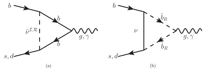
In RPV-MSSMIS, the most favored operator to explain the Bd(s)K()K¯()B_{d(s)}\rightarrow K^{(\ast)}\bar{K}^{(\ast)} puzzle is the magnetic one, 𝒪8gs{\cal O}_{8gs}, extracted from the gluon-penguins shown in Fig. 1. Given the recent LHC constraints which will be discussed in Sec. 3.1, we set all colored SUSY particles with masses above 1010 TeV, so the penguins engaged by squarks and gluinos contribute negligibly.

Next, we will show that, the NP Wilson coefficients C7γpNP{C}_{7\gamma p}^{\rm NP} and C8gpNP{C}_{8gp}^{\rm NP} in RPV-MSSMIS can include the chiral-flip contributions, in the mass-splitting scenario mentioned in Sec.2. The coefficient C8gpNP{C}_{8gp}^{\rm NP}, extracted from the diagrams containing sneutrinos (other suppressed contributions omitted) is given by,

C8gpNP=1482GFηt{\displaystyle{C}_{8gp}^{\rm NP}=-\frac{1}{48\sqrt{2}G_{F}\eta_{t}}\biggl{\{} λvp3λv33mν~v2[8+6log(mb2mν~v2)]λvp3λv33mν~v2[8+6log(mb2mν~v2)]\displaystyle\frac{\lambda^{\prime{\cal I}\ast}_{vp3}\lambda^{\prime{\cal I}\ast}_{v33}}{m_{\tilde{\nu}^{\cal I}_{v}}^{2}}\left[8+6\log\left(\frac{m_{b}^{2}}{m_{\tilde{\nu}^{\cal I}_{v}}^{2}}\right)\right]-\frac{\lambda^{\prime{\cal R}\ast}_{vp3}\lambda^{\prime{\cal R}\ast}_{v33}}{m_{\tilde{\nu}^{\cal R}_{v}}^{2}}\left[8+6\log\left(\frac{m_{b}^{2}}{m_{\tilde{\nu}^{\cal R}_{v}}^{2}}\right)\right]
+λvp3λv33mν~v2+λvp3λv33mν~v2},\displaystyle+\frac{\lambda^{\prime{\cal I}\ast}_{vp3}\lambda^{\prime{\cal I}}_{v33}}{m^{2}_{\tilde{\nu}^{\cal I}_{v}}}+\frac{\lambda^{\prime{\cal R}\ast}_{vp3}\lambda^{\prime{\cal R}}_{v33}}{m^{2}_{\tilde{\nu}^{\cal R}_{v}}}\biggr{\}}, (2.15)

and C7γpNP{C}_{7\gamma p}^{\rm NP} is calculated as C8gp/3-{C}_{8gp}/3 because that in the setup of this model, the difference between bpγbp\gamma diagram and bpgbpg one is merely 1/3-1/3. In Eq. (2.2), ones can find that the chiral-flip is contained in the first two terms containing double-λ\lambda^{\prime\ast} couplings. If we utilize the degenerate-mass scenario, these two terms totally cancel with each other and then only the non-flip terms, λv23λv33/mν~v2+λv23λv33/mν~v2=2λv23λv33/mν~v2{\lambda^{\prime{\cal I}\ast}_{v23}\lambda^{\prime{\cal I}}_{v33}}/{m^{2}_{\tilde{\nu}^{\cal I}_{v}}}+{\lambda^{\prime{\cal R}\ast}_{v23}\lambda^{\prime{\cal R}}_{v33}}/{m^{2}_{\tilde{\nu}^{\cal R}_{v}}}=2{\lambda^{\prime{\cal I}\ast}_{v23}\lambda^{\prime{\cal I}}_{v33}}/{m^{2}_{\tilde{\nu}^{\cal I}_{v}}} are remained, which agrees with the result in Ref. [22], with the formula-sign checked. Instead, if there exists a sufficient split between the masses mν~vm_{\tilde{\nu}^{\cal I}_{v}} and mν~vm_{\tilde{\nu}^{\cal R}_{v}} for the same vv, the unique chiral-flip part is dominating, enhanced by logarithm terms. Here we analyse Fig. 1a qualitatively in the flavor basis to illustrate how double-λ\lambda^{\prime\ast} terms are related to the chiral-flip. First the leading order term only contains normal λλ\lambda^{\prime}\lambda^{\prime\ast} couplings. When we consider the next order with the mixing of chirality for one single virtual quark, the chirality of sneutrino should also be flipped, inducing that double-λ\lambda^{\prime\ast} couplings emerge. This situation is unique since (s)neutrino chiral-flip is forbidden in original RPV-MSSM, with Dirac neutrinos instead of Majorana ones.

Refer to caption
Figure 1: Gluon(phonton)-penguin diagrams in RPV-MSSMIS, within the single-value-kk assumption. The single-value-kk assumption forbids diagrams with charged leptons(sleptons), and squarks with above 1010 TeV masses suppress related diagram contributions.

Then it is worth mentioning that we also calculate the Wilson coefficient C9UNPC^{\rm NP}_{9\rm U} related to the operator, 𝒪9=e216π2(s¯LγμbL)(¯γμ){\cal O}_{9}=\frac{e^{2}}{16\pi^{2}}(\bar{s}_{L}\gamma^{\mu}b_{L})(\bar{\ell}\gamma_{\mu}\ell), which providing the lepton flavor universal contributions to bs+b\rightarrow s\ell^{+}\ell^{-}, also dominated by the ν~dd\tilde{\nu}dd loop. The result is given that,

C9UNP=2144GFηt{\displaystyle C^{\rm NP}_{9\rm U}=-\frac{\sqrt{2}}{144G_{F}\eta_{t}}\biggl{\{} λv23λv33mν~v2[83+2log(mb2mν~v2)]+λv23λv33mν~v2[83+2log(mb2mν~v2)]\displaystyle\frac{\lambda^{\prime{\cal I}\ast}_{v23}\lambda^{\prime{\cal I}}_{v33}}{m_{\tilde{\nu}^{\cal I}_{v}}^{2}}\left[\frac{8}{3}+2\log\left(\frac{m_{b}^{2}}{m_{\tilde{\nu}^{\cal I}_{v}}^{2}}\right)\right]+\frac{\lambda^{\prime{\cal R}\ast}_{v23}\lambda^{\prime{\cal R}}_{v33}}{m_{\tilde{\nu}^{\cal R}_{v}}^{2}}\left[\frac{8}{3}+2\log\left(\frac{m_{b}^{2}}{m_{\tilde{\nu}^{\cal R}_{v}}^{2}}\right)\right]
+λv23λv33mν~v2λv23λv33mν~v2},\displaystyle+\frac{\lambda^{\prime{\cal I}\ast}_{v23}\lambda^{\prime{\cal I}\ast}_{v33}}{m^{2}_{\tilde{\nu}^{\cal I}_{v}}}-\frac{\lambda^{\prime{\cal R}\ast}_{v23}\lambda^{\prime{\cal R}\ast}_{v33}}{m^{2}_{\tilde{\nu}^{\cal R}_{v}}}\biggr{\}}, (2.16)

and ones can find that, the chiral-flip part in Eq. (2.2), expressed by the double-λ\lambda^{\prime\ast} terms, is not enhanced by logarithm terms. In the degenerate-mass scenario, the result returns to the one shown in Ref. [14]. We also examine the ZZ-penguin contribution to C9UNPC^{\rm NP}_{9\rm U}, and find that it is negligible in the setup of this work.

As mentioned in Sec. 1, there are divergences between the experiment data and SM results, corresponding to the non-leptonic ratios LK()K¯()L_{K^{(\ast)}\bar{K}^{(\ast)}}. If we consider NP is only within BsK()K¯()B_{s}\rightarrow K^{(\ast)}\bar{K}^{(\ast)} decays without the BdB_{d} decays, the predictions of the ratios, LK()K¯()L_{K^{(\ast)}\bar{K}^{(\ast)}}, can be given by [2, 13],

LKK¯/LKK¯SM\displaystyle L_{K\bar{K}}/L_{K\bar{K}}^{\rm SM}\approx 1+1.13C8gsNP(μEW)+0.34C8gsNP(μEW)2,\displaystyle 1+1.13C_{8gs}^{\rm NP}(\mu_{\rm EW})+0.34C_{8gs}^{\rm NP}(\mu_{\rm EW})^{2}, (2.17)
LKK¯/LKK¯SM\displaystyle L_{K^{\ast}\bar{K}^{\ast}}/L_{K^{\ast}\bar{K}^{\ast}}^{\rm SM}\approx 1+2.41C8gsNP(μEW)+1.74C8gsNP(μEW)2,\displaystyle 1+2.41C_{8gs}^{\rm NP}(\mu_{\rm EW})+1.74C_{8gs}^{\rm NP}(\mu_{\rm EW})^{2}, (2.18)

where the electroweak (EW) broken scale μEW=160\mu_{\rm EW}=160 GeV. Then at 2σ2\sigma level, we need C8gsNP0.08C_{8gs}^{\rm NP}\lesssim-0.08 to explain the non-leptonic tension. The NP in bdbd sector is constrained very strictly which will be shown in Sec. 3.2.

2.3 BK()νν¯B\rightarrow K^{(\ast)}\nu\bar{\nu} revisited

In this section, we revisit the BK()νν¯B\rightarrow K^{(\ast)}\nu\bar{\nu} processes related to the quark transition djdmνiν¯id_{j}\rightarrow d_{m}\nu_{i}\bar{\nu}_{i^{\prime}}, and the corresponding effective Lagrangian is,

effddνν¯=\displaystyle{\cal L}_{\rm eff}^{dd\nu\bar{\nu}}= (CmjSMδii+CmjNP)(d¯mγμPLdj)(ν¯iγμPLνi)+Cmj1SRR(d¯mPRdj)(ν¯iPRνi)\displaystyle(C^{\rm SM}_{mj}\delta_{ii^{\prime}}+C^{\rm NP}_{mj})(\bar{d}_{m}\gamma_{\mu}P_{L}d_{j})(\bar{\nu}_{i}\gamma^{\mu}P_{L}\nu_{i^{\prime}})+C_{mj}^{\rm 1SRR}(\bar{d}_{m}P_{R}d_{j})(\bar{\nu}_{i}P_{R}\nu_{i^{\prime}})
+Cmj2SRR(d¯mσμνPRdj)(ν¯iσμνPRνi)+h.c.,\displaystyle+C_{mj}^{\rm 2SRR}(\bar{d}_{m}\sigma_{\mu\nu}P_{R}d_{j})(\bar{\nu}_{i}\sigma^{\mu\nu}P_{R}\nu_{i^{\prime}})+{\rm h.c.}, (2.19)

where the SM contribution is CmjSM=2GFe2KtjKtm4π2sin2θWX(xt)C^{\rm SM}_{mj}=-\frac{\sqrt{2}G_{F}e^{2}K_{tj}K^{\ast}_{tm}}{4\pi^{2}\sin^{2}\theta_{W}}X(x_{t}) and the loop function X(xt)xt(xt+2)8(xt1)+3xt(xt2)8(xt1)2log(xt)X(x_{t})\equiv\frac{x_{t}(x_{t}+2)}{8(x_{t}-1)}+\frac{3x_{t}(x_{t}-2)}{8(x_{t}-1)^{2}}\log(x_{t}) with xtmt2/mW2x_{t}\equiv m^{2}_{t}/m^{2}_{W} [23]. The NP contribution of vector current is [15]

CmjNP=λij3𝒩λim3𝒩2mb~R2=𝒱iα𝒱iαλαj3λαm32mb~R2.\displaystyle C^{\rm NP}_{mj}=\frac{\lambda^{\prime\cal N}_{i^{\prime}j3}\lambda^{\prime\cal N\ast}_{im3}}{2m^{2}_{\tilde{b}_{R}}}=\frac{{\cal V}_{i^{\prime}\alpha^{\prime}}{\cal V}^{\ast}_{i\alpha}\lambda^{\prime}_{\alpha^{\prime}j3}\lambda^{\prime\ast}_{\alpha m3}}{2m^{2}_{\tilde{b}_{R}}}. (2.20)

Besides, the NP coefficients Cmj1SRRC_{mj}^{\rm 1SRR} and Cmj2SRRC_{mj}^{\rm 2SRR} express the chiral-flip contributions of neutrino with sbottoms. However, the global fit shows that, these scalar and tensor contributions are negligible, relative to the vector one [24]. For simplicity, we consider negligible mixing for the b~\tilde{b} sector to omit these two coefficients.

To study the NP effects on B+K+νν¯B^{+}\rightarrow K^{+}\nu\bar{\nu} as well as BKνν¯B\rightarrow K^{\ast}\nu\bar{\nu}, ones can define the ratio, RK()νν¯(BK()νν¯)/(BK()νν¯)SMR^{\nu\bar{\nu}}_{K^{(\ast)}}\equiv{{\cal B}(B\rightarrow K^{(\ast)}\nu\bar{\nu})}/{{\cal B}(B\rightarrow K^{(\ast)}\nu\bar{\nu})_{\rm SM}}. In RPV-MSSMIS, we get that,

RKνν¯=RKνν¯=i=13|C23SM+C23NP|2+ii3|C23NP|23|C23SM|2.\displaystyle R^{\nu\bar{\nu}}_{K}=R^{\nu\bar{\nu}}_{K^{\ast}}=\frac{\sum\limits_{i=1}^{3}\left|C_{23}^{\rm SM}+C_{23}^{\rm NP}\right|^{2}+\sum\limits_{i\neq i^{\prime}}^{3}\left|C_{23}^{\rm NP}\right|^{2}}{3\left|C_{23}^{\rm SM}\right|^{2}}. (2.21)

The recent Belle-II data [16] of BK+νν¯B\rightarrow K^{+}\nu\bar{\nu}, and the updated SM prediction [17], induce RKνν¯=5.3±1.7R^{\nu\bar{\nu}}_{K}=5.3\pm 1.7 [25]. Recent research [25] shows that, the case of RKνν¯=RKνν¯R^{\nu\bar{\nu}}_{K}=R^{\nu\bar{\nu}}_{K^{\ast}} cannot simultaneously fulfill the Belle-II data at 1σ1\sigma level as well as the upper limit (BKνν¯)exp<1.8×10⁵{\cal B}(B\rightarrow K^{\ast}\nu\bar{\nu})_{\rm exp}<1.8\times 10^{-5} [26], i.e. RKνν¯<1.9R^{\nu\bar{\nu}}_{K^{\ast}}<1.9, at 90%90\% confidence level (CL). Besides, with the theoretical result (B+K+νν¯)/(BKνν¯)0.4{\cal B}(B^{+}\rightarrow K^{+}\nu\bar{\nu})/{\cal B}(B\rightarrow K^{\ast}\nu\bar{\nu})\approx 0.4 for the single left-handed vector operator, it is also found that this case cannot explain the Belle-II data, without staying below the upper limit of (BKνν¯){\cal B}(B\rightarrow K^{\ast}\nu\bar{\nu}) at 90%90\% CL [27, 28]. In this work, we will investigate the degree of RKνν¯R^{\nu\bar{\nu}}_{K} approaching to its upper limit 1.91.9, in the parameter space of RPV-MSSMIS.

3 The constraints

Before the numerical analysis of Bd(s)K()K¯()B_{d(s)}\rightarrow K^{(\ast)}\bar{K}^{(\ast)} puzzle, the relevant experimental constraints should also be scrutinised.

3.1 Direct searches

Firstly, direct searches for SUSY particles should be considered. Since there are no signs of NP particles until the end of the LHC run II which reaching around 140140 fb-1 at the center energy 1313 TeV, which providing stringent bounds on SUSY models. The allowed masses of colored sparticles, such as gluinos, the first-two generation squarks, stops and sbottoms have been excluded up to 121-2 TeV scale [29, 30, 31, 32, 33, 34, 35]. In this work, the masses of all the colored SUSY particles are set above 1010 TeV, whereas the masses of sleptons as well as the heavy neutrinos are all around 10210310^{2}-10^{3} GeV. Some recent experiments have pushed the upper limit of slepton masses over TeV scale [36, 37, 38], however, these searches consider nonzero λ\lambda related to the superpotential λijkL^iL^jE^k\lambda_{ijk}\hat{L}_{i}\hat{L}_{j}\hat{E}_{k}. Given that we only consider nonzero λ\lambda^{\prime} in the model, this bound can be relaxed . It is worth mentioning that, ATLAS has recently made searches for the NP signs of this type of model, only containing λ\lambda^{\prime} couplings [39]. Using the first collider limits for this model type, we keep mμ~470m_{\tilde{\mu}}\gtrsim 470 GeV.

3.2 Tree-level processes

Next, we check the tree-level processes exchanging sbottoms, including K+π+νν¯K^{+}\to\pi^{+}\nu\bar{\nu}, Bπνν¯B\to\pi\nu\bar{\nu}, D0+D^{0}\to\ell^{+}\ell^{-}, τρ0\tau\rightarrow\ell\rho^{0} as well as BτνB\to\tau\nu, DsτνD_{s}\to\tau\nu, τK(π)ν\tau\to K(\pi)\nu and πν(γ)\pi\to\ell\nu(\gamma).

As ones know that the experimental measurement (K+π+νν¯)exp=(1.140.33+0.40)×1010{\cal B}(K^{+}\to\pi^{+}\nu\bar{\nu})_{\rm exp}=(1.14^{+0.40}_{-0.33})\times 10^{-10} [40] and the SM prediction (K+π+νν¯)SM=(9.24±0.83)×1011{\cal B}(K^{+}\to\pi^{+}\nu\bar{\nu})_{\rm SM}=(9.24\pm 0.83)\times 10^{-11} [41] induce the strong constraint, |λi2k𝒩λi1k𝒩|104(mb~R/1TeV)2|\lambda^{\prime\cal N}_{i^{\prime}2k}\lambda^{\prime\cal N\ast}_{i1k}|\lesssim 10^{-4}(m_{\tilde{b}_{R}}/1{\rm TeV})^{2}. Even for b~R{\tilde{b}_{R}} with 1010 TeV mass, there still exists the bound of |λi2k𝒩λi1k𝒩|0.01|\lambda^{\prime\cal N}_{i^{\prime}2k}\lambda^{\prime\cal N\ast}_{i1k}|\lesssim 0.01. Thus, we assume λi1k\lambda^{\prime}_{i1k} negligible to avoid this bound from this process, as well as the Bπνν¯B\to\pi\nu\bar{\nu} decay.

In table 1, we collect the experimental results and SM predictions of D0+D^{0}\to\ell^{+}\ell^{-}, τρ0\tau\rightarrow\ell\rho^{0} decays with the charged current processes, BτνB\to\tau\nu, DsτνD_{s}\to\tau\nu and τKν\tau\to K\nu, as well as the processes discussed above. Following the same/analogical numerical calculations in the ordinary RPV-MSSM (see Refs. [42, 43]), we update the constraint from (D0μ+μ){\cal B}(D^{0}\to\mu^{+}\mu^{-}), as |λ223|2<0.22(mb~R/1TeV)2|\lambda^{\prime}_{223}|^{2}<0.22(m_{\tilde{b}_{R}}/1{\rm TeV})^{2}, and the bound from (D0e+e){\cal B}(D^{0}\to e^{+}e^{-}) is negligible due to the small mem_{e}. We also update the calculation of the process (τρ0){\cal B}(\tau\rightarrow\ell\rho^{0}), which provides the bound |λ323λ223|<0.45(mb~R/1TeV)2|\lambda^{\prime}_{323}\lambda^{\prime\ast}_{223}|<0.45(m_{\tilde{b}_{R}}/1{\rm TeV})^{2} as well as |λ323λ123|<0.51(mb~R/1TeV)2|\lambda^{\prime}_{323}\lambda^{\prime\ast}_{123}|<0.51(m_{\tilde{b}_{R}}/1{\rm TeV})^{2}. The functions R133R_{133}, R223R_{223}, and R123R_{123} (see concrete definitions in Ref. [43]), are utilized to express the ratios of the measurement values versus the SM predictions for (Bτν){\cal B}(B\to\tau\nu), (Dsτν){\cal B}(D_{s}\to\tau\nu), and (τKν){\cal B}(\tau\to K\nu), respectively, and we also consider these constraints.

As for the πν(γ)\pi\to\ell\nu(\gamma) decay, similar to the formula in Ref. [44], the bound (here also including λ\lambda^{\prime}-loop corrections) can be shown with

1+ημμ+hμμ1+ηee+hee=1.0010(9),\displaystyle\frac{1+\eta_{\mu\mu}+h^{\prime}_{\mu\mu}}{1+\eta_{ee}+h^{\prime}_{ee}}=1.0010(9), (3.1)

where the function η\eta and hh^{\prime} express the non-unitary part of neutrino and λ\lambda^{\prime}-loop corrections to WlνWl\nu-vertex, respectively, and they are given by  [15]

ηij\displaystyle\eta_{ij}\equiv (𝒱3×3T)ik𝒰kj1δij,\displaystyle\left({\cal V}^{T}_{3\times 3}\right)_{ik}{\cal U}^{-1}_{kj}-\delta_{ij},
hli=\displaystyle h^{\prime}_{li}= 364π2xb~RfW(xb~R)λ~l33λ~i33,\displaystyle-\frac{3}{64\pi^{2}}x_{\tilde{b}_{R}}f_{W}(x_{\tilde{b}_{R}})\tilde{\lambda}^{\prime\ast}_{l33}\tilde{\lambda}^{\prime}_{i33}, (3.2)

where 𝒰{\cal U} is unitary PMNS-like, and the loop function fW(x)1x1+(x2)logx(x1)2f_{W}(x)\equiv\frac{1}{x-1}+\frac{(x-2)\log x}{(x-1)^{2}} with xb~Rmt2/mb~R2x_{\tilde{b}_{R}}\equiv m^{2}_{t}/m^{2}_{\tilde{b}_{R}}, from the dominant uidib~Ru_{i}d_{i}\tilde{b}_{R}-loop diagram. In the inverse seesaw framework, the Hermitian η\eta can be figured out, i.e. η12mD(MR)1(MRT)1mD\eta\approx-\frac{1}{2}m_{D}^{\dagger}(M_{R}^{\ast})^{-1}(M_{R}^{T})^{-1}m_{D}. We can translate the bound Eq. (3.1) into |ηee+hee|0.0028|\eta_{ee}+h^{\prime}_{ee}|\lesssim 0.0028 at the 2σ2\sigma level, with the negligible η(h)μμ\eta(h^{\prime})_{\mu\mu}. In this work, we can set sufficiently small λ2jk\lambda^{\prime}_{2jk} to keep hμμh^{\prime}_{\mu\mu} (negative as well as ημμ\eta_{\mu\mu}) negligible to avoid enlarging the Cabbibo anomaly [45, 46].

In RPV-MSSMIS, the neutrino mixing matrix, 𝒱{\cal V}, is also bounded by the τ(μ)\tau(\mu) decaying to charged leptons and neutrinos at the tree level. However, at one-loop level, both 𝒱{\cal V} and λ\lambda^{\prime} couplings are constrained by these decays as well as the charged lepton flavor violating (cLFV) decays. We will address τ(μ)\tau(\mu) decays totally in the following subsection 3.3, and before that, we can make a summary that couplings λi13\lambda^{\prime}_{i13} and λ2j3\lambda^{\prime}_{2j3} are already set negligible (at μNP\mu_{\rm NP} scale), considering the constraints investigated above, and that is, NP is mainly not contained in the dd and μ\mu sectors.

Observations SM predictions Experimental data
(K+π+νν¯){\cal B}(K^{+}\to\pi^{+}\nu\bar{\nu}) (9.24±0.83)×1011(9.24\pm 0.83)\times 10^{-11} [41] (1.140.33+0.40)×1010(1.14^{+0.40}_{-0.33})\times 10^{-10} [40]
(D0μ+μ){\cal B}(D^{0}\to\mu^{+}\mu^{-}) 6×10¹¹\lesssim 6\times 10^{-11} [47] <3.1×10⁹<3.1\times 10^{-9} [48]
(τeρ0){\cal B}(\tau\rightarrow e\rho^{0}) - <2.2×10⁸<2.2\times 10^{-8} [49]
(τμρ0){\cal B}(\tau\rightarrow\mu\rho^{0}) - <1.7×10⁸<1.7\times 10^{-8} [49]
(Bτν){\cal B}(B\to\tau\nu) (9.47±1.82)×105(9.47\pm 1.82)\times 10^{-5} [50] (1.09±0.24)×104(1.09\pm 0.24)\times 10^{-4} [40]
(Dsτν){\cal B}(D_{s}\to\tau\nu) (5.40±0.30)%(5.40\pm 0.30)\% [43] (5.36±0.10)%(5.36\pm 0.10)\% [40]
(τKν){\cal B}(\tau\to K\nu) (7.15±0.026)×103(7.15\pm 0.026)\times 10^{-3} [51] (6.96±0.10)×103(6.96\pm 0.10)\times 10^{-3} [40]
Table 1: Current status of the relevant processes which can be affected by RPV-MSSMIS at tree level. The experimental upper limits are given at 90%90\% CL.

3.3 Loop-level processes

In this section illustrating loop-level bounds, we firstly investigate the BsB¯sB_{s}-\bar{B}_{s} mixing, which is mastered by

effbs¯bs¯=(CSMVLL+CNPVLL)(s¯γμPLb)(s¯γμPLb)+CNP1SRR(s¯PRb)(s¯PRb)+h.c.,\displaystyle{\cal L}_{\rm eff}^{b\bar{s}b\bar{s}}=(C^{\rm VLL}_{\rm SM}+C^{\rm VLL}_{\rm NP})(\bar{s}\gamma_{\mu}P_{L}b)(\bar{s}\gamma^{\mu}P_{L}b)+C^{\rm 1SRR}_{\rm NP}(\bar{s}P_{R}b)(\bar{s}P_{R}b)+{\rm h.c.}, (3.3)

where the SM contribution is CBsSM=14π2GF2mW2ηt2S(xt)C_{B_{s}}^{\rm SM}=-\frac{1}{4\pi^{2}}G_{F}^{2}m_{W}^{2}\eta_{t}^{2}S(x_{t}) with the defined function S(xt)xt(411xt+xt2)4(xt1)2+3xt3log(xt)2(xt1)3S(x_{t})\equiv\frac{x_{t}(4-11x_{t}+x_{t}^{2})}{4(x_{t}-1)^{2}}+\frac{3x_{t}^{3}\log(x_{t})}{2(x_{t}-1)^{3}}, and the non-negligible NP contributions are,

CNPVLL\displaystyle C_{\rm NP}^{\rm VLL} =18i(14Λvv1𝒳𝒴D2[mν~v𝒳,mν~v𝒴,mb,mb]+Λvv𝒩D2[mνv,mνv,mb~R,mb~R]),\displaystyle=\frac{1}{8i}\bigl{(}\frac{1}{4}\Lambda^{\prime 1\cal XY}_{vv^{\prime}}D_{2}[m_{\tilde{\nu}^{\cal X}_{v}},m_{\tilde{\nu}^{\cal Y}_{v^{\prime}}},m_{b},m_{b}]+\Lambda^{\prime\cal N}_{vv^{\prime}}D_{2}[m_{\nu_{v}},m_{\nu_{v^{\prime}}},m_{\tilde{b}_{R}},m_{\tilde{b}_{R}}]\bigr{)},
CNP1SRR\displaystyle C_{\rm NP}^{\rm 1SRR} =18i(Λvv2𝒳𝒴(1)δ𝒳𝒴+1mb2D0[mν~v𝒳,mν~v𝒴,mb,mb]\displaystyle=\frac{1}{8i}\bigl{(}\Lambda^{\prime 2\cal XY}_{vv^{\prime}}(-1)^{\delta_{\cal XY}+1}m_{b}^{2}D_{0}[m_{\tilde{\nu}^{\cal X}_{v}},m_{\tilde{\nu}^{\cal Y}_{v^{\prime}}},m_{b},m_{b}]
+Λvv3𝒳𝒴(δ𝒳δ𝒳)mb2D0[mν~v𝒳,mν~v𝒴,mb,mb]Λvv1𝒳𝒴mb2D1[mν~v𝒳,mν~v𝒴,mb,mb]\displaystyle+\Lambda^{\prime 3\cal XY}_{vv^{\prime}}(\delta_{\cal XR}-\delta_{\cal XI})m_{b}^{2}D_{0}[m_{\tilde{\nu}^{\cal X}_{v}},m_{\tilde{\nu}^{\cal Y}_{v^{\prime}}},m_{b},m_{b}]-\Lambda^{\prime 1\cal XY}_{vv^{\prime}}m_{b}^{2}D_{1}[m_{\tilde{\nu}^{\cal X}_{v}},m_{\tilde{\nu}^{\cal Y}_{v^{\prime}}},m_{b},m_{b}]
+Λvv4𝒳𝒴(δ𝒴δ𝒴)mb2D1[mν~v𝒳,mν~v𝒴,mb,mb]λv2322mν~v2+λv2322mν~v2),\displaystyle+\Lambda^{\prime 4\cal XY}_{vv^{\prime}}(\delta_{\cal YI}-\delta_{\cal YR})m_{b}^{2}D_{1}[m_{\tilde{\nu}^{\cal X}_{v}},m_{\tilde{\nu}^{\cal Y}_{v^{\prime}}},m_{b},m_{b}]-\frac{\lambda^{\prime{\cal I}\ast 2}_{v23}}{2m^{2}_{\tilde{\nu}^{\cal I}_{v}}}+\frac{\lambda^{\prime{\cal R}\ast 2}_{v23}}{2m^{2}_{\tilde{\nu}^{\cal R}_{v}}}\bigr{)}, (3.4)

where Λvv1𝒳𝒴λv33𝒳λv23𝒳λv33𝒴λv23𝒴\Lambda^{\prime 1\cal XY}_{vv^{\prime}}\equiv\lambda^{\prime\cal X}_{v33}\lambda^{\prime\cal X\ast}_{v23}\lambda^{\prime\cal Y}_{v^{\prime}33}\lambda^{\prime\cal Y\ast}_{v^{\prime}23}, Λvv2𝒳𝒴λv33𝒳λv23𝒳λv33𝒴λv23𝒴\Lambda^{\prime 2\cal XY}_{vv^{\prime}}\equiv\lambda^{\prime\cal X\ast}_{v33}\lambda^{\prime\cal X\ast}_{v23}\lambda^{\prime\cal Y\ast}_{v^{\prime}33}\lambda^{\prime\cal Y\ast}_{v^{\prime}23}, Λvv3𝒳𝒴λv33𝒳λv23𝒳λv33𝒴λv23𝒴\Lambda^{\prime 3\cal XY}_{vv^{\prime}}\equiv\lambda^{\prime\cal X\ast}_{v33}\lambda^{\prime\cal X\ast}_{v23}\lambda^{\prime\cal Y}_{v^{\prime}33}\lambda^{\prime\cal Y\ast}_{v^{\prime}23}, and Λvv4𝒳𝒴λv33𝒳λv23𝒳λv33𝒴λv23𝒴\Lambda^{\prime 4\cal XY}_{vv^{\prime}}\equiv\lambda^{\prime\cal X}_{v33}\lambda^{\prime\cal X\ast}_{v23}\lambda^{\prime\cal Y\ast}_{v^{\prime}33}\lambda^{\prime\cal Y\ast}_{v^{\prime}23} with 𝒳{\cal X}, 𝒴{\cal Y} being {\cal I} or {\cal R}, and Λvv𝒩λv33𝒩λv23𝒩λv33𝒩λv23𝒩\Lambda^{\prime\cal N}_{vv^{\prime}}\equiv\lambda^{\prime\cal N}_{v33}\lambda^{\prime\cal N\ast}_{v23}\lambda^{\prime\cal N}_{v^{\prime}33}\lambda^{\prime\cal N\ast}_{v^{\prime}23}. The formulas of Passarino-Veltman functions [52], D0D_{0} and D2D_{2}, are defined as

D0[m1,m2,m3,m4]\displaystyle D_{0}[m_{1},m_{2},m_{3},m_{4}]\equiv d4k(2π)41(k2m12)(k2m22)(k2m32)(k2m42),\displaystyle\int\frac{d^{4}k}{(2\pi)^{4}}\frac{1}{(k^{2}-m_{1}^{2})(k^{2}-m_{2}^{2})(k^{2}-m_{3}^{2})(k^{2}-m_{4}^{2})},
D2[m1,m2,m3,m4]\displaystyle D_{2}[m_{1},m_{2},m_{3},m_{4}]\equiv d4k(2π)4k2(k2m12)(k2m22)(k2m32)(k2m42),\displaystyle\int\frac{d^{4}k}{(2\pi)^{4}}\frac{k^{2}}{(k^{2}-m_{1}^{2})(k^{2}-m_{2}^{2})(k^{2}-m_{3}^{2})(k^{2}-m_{4}^{2})}, (3.5)

and D1D_{1} is given by Dμ=piμDiD_{\mu}=p_{i\mu}D_{i} [53], which is defined as

Dμd4k(2π)4kμ(k2m12)((k+p1)2m22)((k+p2)2m32)((k+p3)2m42),\displaystyle D_{\mu}\equiv\int\frac{d^{4}k}{(2\pi)^{4}}\frac{k_{\mu}}{(k^{2}-m_{1}^{2})((k+p_{1})^{2}-m_{2}^{2})((k+p_{2})^{2}-m_{3}^{2})((k+p_{3})^{2}-m_{4}^{2})}, (3.6)

with the limit pipj0p_{i}\cdot p_{j}\rightarrow 0 applied. The chiral-flip contributions are all contained in the coefficient CNP1SRRC_{\rm NP}^{\rm 1SRR}, where the last two terms are extracted from the tree-level diagram. Combined with recent results of bag parameters, Bs(i)(mb)B_{s}^{(i)}(m_{b}), including the new value of Bs(1)(mb)B_{s}^{(1)}(m_{b}) [54, 55], we get the ratio,

BsΔMsΔMsSM=|1+CNPVLLCSMVLL2.38CNP1SRRCSMVLL|.\displaystyle{\cal R}_{B_{s}}\equiv\frac{\Delta M_{s}}{\Delta M_{s}^{\rm SM}}=\left|1+\frac{C^{\rm VLL}_{\rm NP}}{C^{\rm VLL}_{\rm SM}}-2.38\frac{C_{\rm NP}^{\rm 1SRR}}{C^{\rm VLL}_{\rm SM}}\right|. (3.7)

The recent result averaged by HFLAV, ΔMsexp=(17.765±0.006)\Delta M_{s}^{\rm exp}=(17.765\pm 0.006) ps1{\rm ps}^{-1} [56], along with the SM prediction ΔMsSM=(18.23±0.63)ps1\Delta M_{s}^{\rm SM}=(18.23\pm{0.63})~{}{\rm ps}^{-1} [57], leads to the strong constraint 0.90<Bs<1.040.90<{\cal R}_{B_{s}}<1.04 at 2σ2\sigma level. Given that the mass-splitting of sneutrinos is considered in this work, the tree-level contributions to the ratio Bs{\cal R}_{B_{s}} need the cancellation to fulfill the bound.

Next we investigate the cLFV processes, i.e. τγ\tau\to\ell\gamma, μeγ\mu\to e\gamma, τ()\tau\to\ell^{(^{\prime})}\ell\ell (\ell^{\prime}\neq\ell) and μeee\mu\to eee. It should be stressed that the NP contributions from neutrino part, can be eliminated with the particular structures of (s)neutrino mass matrices. We utilize the structures where only chiral mixing but no flavor mixing exists for the neutrino sector involving right-handed (RH) neutrinos, as well as the whole sneutrino sector (see detailed discussions in Ref. [14] and appendix A). Then, we focus on the λ\lambda^{\prime} contributions. The branching fraction of the τγ\tau\to\ell\gamma decay is given by [58]

(τγ)=τταmτ54(|A2L|2+|A2R|2),\displaystyle{\cal B}(\tau\to\ell\gamma)=\frac{\tau_{\tau}\alpha m^{5}_{\tau}}{4}(|A^{L}_{2}|^{2}+|A^{R}_{2}|^{2}), (3.8)

where the effective couplings A2L=λj3λ3j3/64π2mb~R2A^{L}_{2}=-{\lambda^{\prime}_{\ell j3}\lambda^{\prime\ast}_{3j3}}/{64\pi^{2}m^{2}_{\tilde{b}_{R}}} and A2R=0A^{R}_{2}=0, with the limit of m2/mτ20m^{2}_{\ell}/m^{2}_{\tau}\to 0 adopted here as well as the other cLFV processes. Because λ2jk\lambda^{\prime}_{2jk} is already set negligible, processes μeγ\mu\to e\gamma, μeee\mu\to eee, τμγ\tau\to\mu\gamma, τμμμ\tau\to\mu\mu\mu, and τ\tau\to\ell^{{}^{\prime}}\ell\ell, will not make effective bounds. Then the remained ones to be considered are τeγ\tau\to e\gamma and τeee\tau\to eee decays (see the relevant formulas in Ref. [43]), with the experimental upper limits (τeγ)exp<3.3×10⁸{\cal B}(\tau\to e\gamma)_{\rm exp}<3.3\times 10^{-8} and (τeee)exp<2.7×10⁸{\cal B}(\tau\to eee)_{\rm exp}<2.7\times 10^{-8} at 90%90\% CL, respectively [40].

Following the introduction of cLFV, we will mention the BXsγB\to X_{s}\gamma decay, which are mastered by the electromagnetic dipole C7γsC8gs/3C_{7\gamma s}\approx-C_{8gs}/3 as well as C8gsC_{8gs}. Although the recent SM prediction (BXsγ)SM×104=3.40±0.17{\cal B}(B\rightarrow X_{s}\gamma)_{\rm SM}\times 10^{4}=3.40\pm 0.17 (Eγ>1.6E_{\gamma}>1.6 GeV) [60], agrees very well with the recent measured branching ratio (BXsγ)exp×104=3.32±0.15{\cal B}(B\rightarrow X_{s}\gamma)_{\rm exp}\times 10^{4}=3.32\pm 0.15 [61], which implies a very strict constraint, both contributions to this branching ratio from C7γsC_{7\gamma s} and C8gsC_{8gs} can counteract each other partly, shown as (BXsγ)×104=(3.40±0.17)8.25C7γs(μEW)2.10C8gs(μEW){\cal B}(B\rightarrow X_{s}\gamma)\times 10^{4}=(3.40\pm 0.17)-8.25C_{7\gamma s}(\mu_{\rm EW})-2.10C_{8gs}(\mu_{\rm EW}) [60], so RPV-MSSMIS can avoid this stringent bound, given the value of C8gs(μEW)C_{8gs}(\mu_{\rm EW}) is expected around 0.1-0.1 (inducing C7γs(μEW)0.03C_{7\gamma s}(\mu_{\rm EW})\approx 0.03) for explaining non-leptonic puzzle.

In the following, we move on to the purely leptonic decays of ZZ, WW bosons. The effective Lagrangian of ZZ-boson interaction to generic fermions fi,jf_{i,j} is given by [62]

effZff=ecosθWsinθWf¯iγμ(gfLijPL+gfRijPR)fjZμ,\displaystyle{\cal L}^{Zff}_{\rm eff}=\frac{e}{\cos\theta_{W}\sin\theta_{W}}\bar{f}_{i}\gamma^{\mu}\left(g_{f_{L}}^{ij}P_{L}+g_{f_{R}}^{ij}P_{R}\right)f_{j}Z_{\mu}, (3.9)

where gfLij=δijgfLSM+δgfLijg_{f_{L}}^{ij}=\delta^{ij}g_{f_{L}}^{\rm SM}+\delta g_{f_{L}}^{ij} and gfRij=δijgfRSM+δgfRijg_{f_{R}}^{ij}=\delta^{ij}g_{f_{R}}^{\rm SM}+\delta g_{f_{R}}^{ij}. We first investigate Zlilj+Z\rightarrow l^{-}_{i}l^{+}_{j} decay, and the relevant couplings, glLSM=12+sin2θWg_{l_{L}}^{\rm SM}=-\frac{1}{2}+\sin^{2}\theta_{W} and glRSM=sin2θWg_{l_{R}}^{\rm SM}=\sin^{2}\theta_{W}. In the limit of mli/mZ0m_{l_{i}}/m_{Z}\to 0, the corresponding branching fractions are

(Zlilj+)=mZ36πv2ΓZ(|glLij|2+|glRij|2),\displaystyle{\cal B}(Z\to l^{-}_{i}l^{+}_{j})=\frac{m^{3}_{Z}}{6\pi v^{2}\Gamma_{Z}}\left(|g_{l_{L}}^{ij}|^{2}+|g_{l_{R}}^{ij}|^{2}\right), (3.10)

with ZZ-width ΓZ=2.4955\Gamma_{Z}=2.4955 GeV [40]. For iji\neq j, the branching ratio should be given by [(Zlilj+)+(Zljli+)]/2[{\cal B}(Z\to l^{-}_{i}l^{+}_{j})+{\cal B}(Z\to l^{-}_{j}l^{+}_{i})]/2. The NP effective couplings, contributed mainly by λ\lambda^{\prime} effects, are expressed as δglLij=132π2Bij\delta g_{l_{L}}^{ij}=\frac{1}{32\pi^{2}}B^{ij} (δglRij=0\delta g_{l_{R}}^{ij}=0) here and the formulas of BijB^{ij} functions are given by [42],

B1ij=\displaystyle B^{ij}_{1}= 3λ~j33λ~i33{xb~R(1+logxb~R)+mZ218mb~R2[(1110sin2θW)\displaystyle 3\tilde{\lambda}^{\prime}_{j33}\tilde{\lambda}^{\prime\ast}_{i33}\biggl{\{}-x_{\tilde{b}_{R}}(1+\log x_{\tilde{b}_{R}})+\frac{m_{Z}^{2}}{18m^{2}_{\tilde{b}_{R}}}\biggl{[}(11-10\sin^{2}\theta_{W})
+(68sin2θW)logxb~R+110(9+16sin2θW)mZ2mt2]},\displaystyle+(6-8\sin^{2}\theta_{W})\log x_{\tilde{b}_{R}}+\frac{1}{10}(-9+16\sin^{2}\theta_{W})\frac{m_{Z}^{2}}{m_{t}^{2}}\biggr{]}\biggl{\}},
B2ij=\displaystyle B^{ij}_{2}= =12λ~j3λ~i3mZ2mb~R2[(143sin2θW)(logmZ2mb~R2iπ13)+sin2θW9].\displaystyle\sum_{\ell=1}^{2}\tilde{\lambda}^{\prime}_{j\ell 3}\tilde{\lambda}^{\prime\ast}_{i\ell 3}\frac{m_{Z}^{2}}{m^{2}_{\tilde{b}_{R}}}\biggl{[}(1-\frac{4}{3}\sin^{2}\theta_{W})(\log\frac{m_{Z}^{2}}{m^{2}_{\tilde{b}_{R}}}-i\pi-\frac{1}{3})+\frac{\sin^{2}\theta_{W}}{9}\biggr{]}. (3.11)

With the data of the partial width ratios of ZZ bosons, i.e. Γ(Zμμ)/Γ(Zee)=1.0001(24)\Gamma(Z\to\mu\mu)/\Gamma(Z\to ee)=1.0001(24), Γ(Zττ)/Γ(Zμμ)=1.0010(26)\Gamma(Z\to\tau\tau)/\Gamma(Z\to\mu\mu)=1.0010(26) and Γ(Zττ)/Γ(Zee)=1.0020(32)\Gamma(Z\to\tau\tau)/\Gamma(Z\to ee)=1.0020(32) [40], we have the bound of |B11|<0.36|B^{11}|<0.36 with |B33|<0.32|B^{33}|<0.32. And the upper limit of branching ratio, B(Zeτ)<9.8×10⁶{\cal}B(Z\to e\tau)<9.8\times 10^{-6} at 95%95\% CL [40], makes the bound |B13|2+|B31|2<1.42|B^{13}|^{2}+|B^{31}|^{2}<1.4^{2}.

Then we study the invisible ZZ-decays, i.e. ZZ boson interaction to neutrinos, mainly in this model. The effective number of light neutrinos NνN_{\nu}, defined by Γinv=NνΓνν¯SM\Gamma_{\rm inv}=N_{\nu}\Gamma_{\nu\bar{\nu}}^{\rm SM} [63], will constrain the relevant couplings gνg_{\nu} in Eq. (3.9), via

Nν=i,j|δij+δgνijδgνSM|2,\displaystyle N_{\nu}=\sum_{i,j}\left|\delta_{ij}+\frac{\delta g_{\nu}^{ij}}{\delta g_{\nu}^{\rm SM}}\right|^{2}, (3.12)

where the coupling δgνSM=12\delta g_{\nu}^{\rm SM}=\frac{1}{2} and the formulas of δgν()ij\delta g_{\nu}^{(\prime)ij} is given by [64]

(32π2)δgνij=\displaystyle(32\pi^{2})\delta g_{\nu}^{ij}= λj33λi33mZ2mb~R2[(1+23sin2θW)(log(mZ2mb~R2)iπ13)+(112+49sin2θW)].\displaystyle\lambda^{\prime}_{j33}\lambda^{\prime\ast}_{i33}\frac{m^{2}_{Z}}{m^{2}_{\tilde{b}_{R}}}\biggl{[}\left(-1+\frac{2}{3}\sin^{2}\theta_{W}\right)\left(\log\left(\frac{m^{2}_{Z}}{m^{2}_{\tilde{b}_{R}}}\right)-i\pi-\frac{1}{3}\right)+\left(-\frac{1}{12}+\frac{4}{9}\sin^{2}\theta_{W}\right)\biggr{]}. (3.13)

Then the measurement result Nνexp=2.9840(82)N_{\nu}^{\rm exp}=2.9840(82) [63] will make constraints.

As for the purely leptonic decays of WW boson, they can be covered by the stronger ones from μeν¯eνμ\mu\to e\bar{\nu}_{e}\nu_{\mu} and τν¯ντ\tau\to\ell\bar{\nu}_{\ell}\nu_{\tau} decays. The fraction ratios of these lepton decays, i.e. (τμν¯μντ)/(τeν¯eντ){\cal B}(\tau\to\mu\bar{\nu}_{\mu}\nu_{\tau})/{\cal B}(\tau\to e\bar{\nu}_{e}\nu_{\tau}), (τeν¯eντ)/(μeν¯eνμ){\cal B}(\tau\to e\bar{\nu}_{e}\nu_{\tau})/{\cal B}(\mu\to e\bar{\nu}_{e}\nu_{\mu}) and (τμν¯μντ)/(μeν¯eνμ){\cal B}(\tau\to\mu\bar{\nu}_{\mu}\nu_{\tau})/{\cal B}(\mu\to e\bar{\nu}_{e}\nu_{\mu}), make the bounds [44] on the model parameters, which can be expressed as

1+ημμ1+ηee+hee\displaystyle\frac{1+\eta_{\mu\mu}}{1+\eta_{ee}+h^{\prime}_{ee}} =1.0018(14),\displaystyle=1.0018(14),
1+ηττ+hττ1+ημμ\displaystyle\frac{1+\eta_{\tau\tau}+h^{\prime}_{\tau\tau}}{1+\eta_{\mu\mu}} =1.0010(14),\displaystyle=1.0010(14),
1+ηττ+hττ1+ηee+hee\displaystyle\frac{1+\eta_{\tau\tau}+h^{\prime}_{\tau\tau}}{1+\eta_{ee}+h^{\prime}_{ee}} =1.0029(14).\displaystyle=1.0029(14). (3.14)

Here we only consider the WlνlWl\nu_{l}-vertex, which has the interference with the SM contribution, and the LFV-vertex WlνlWl\nu_{l^{\prime}} and ZllZll^{\prime}, which can be embedded in llνi¯νjl\to l^{\prime}\bar{\nu_{i}}\nu_{j} process, are omitted. With the last two formulas of Eq. (3.3) combined with |ημμ|104|\eta_{\mu\mu}|\lesssim 10^{-4}, we should keep |ηττ+hττ|0.0018|\eta_{\tau\tau}+h^{\prime}_{\tau\tau}|\lesssim 0.0018 and |ηττ+hττ||ηee+hee||\eta_{\tau\tau}+h^{\prime}_{\tau\tau}|\lesssim|\eta_{ee}+h^{\prime}_{ee}| at 2σ2\sigma level.

At last, we scrutinize all the one-loop level diagrams of bs+b\rightarrow s\ell^{+}\ell^{-} to search for the potential chiral-flip contributions. The Wilson coefficients C9UNPC^{\rm NP}_{\rm 9U} and C9NP=C10NPC^{\rm NP}_{\rm 9\ell}=-C^{\rm NP}_{\rm 10\ell} (see definitions in Ref. [15]) are calculated and compared with the results of degenerate-mass scenario [14].

4 Numerical analyses

In this section, we begin to analyse Bd(s)K()K¯()B_{d(s)}\rightarrow K^{(\ast)}\bar{K}^{(\ast)} and B+K+νν¯B^{+}\rightarrow K^{+}\nu\bar{\nu} numerically within the mass-splitting scenario of RPV-MSSMIS. We consider normal ordering and δCP=π\delta_{\rm CP}=\pi with the recent data of neutrino oscillation [65]. Then it can be calculated that the three light neutrinos have masses {0,0.008,0.05}\{0,0.008,0.05\} eV with mνl{0,Δm212,Δm312}m_{\nu_{l}}\approx\{0,\sqrt{\Delta m^{2}_{21}},\sqrt{\Delta m^{2}_{31}}\} [66]. The sets of model parameters are collected in table 2.

The diagonal inputs of YνY_{\nu}, MRM_{R}, mL~m_{\tilde{L}^{\prime}}, BMRB_{M_{R}}, and BμSB_{\mu_{S}} here can induce no flavor mixings in sneutrino sector, as well as the neutrino sector which RH neutrinos engage in, and this is benefit for fulfilling the bounds of cLFV decays. Besides, the input values shown in table 2 can induce a diagonal η=diag(1.18,0.18,0.15)×103\eta=-\text{diag}(1.18,0.18,0.15)\times 10^{-3}, which induces the WW mass prediction MW80.385M_{W}\approx 80.385 GeV, fulfilling the recent data [40]. The values of mL~im_{\tilde{L}^{\prime}_{i}} induce physical mass of the lightest sneutrino, as mν~1270m_{\tilde{\nu}_{1}}\approx 270 GeV, allowed by the relevant constraints [40] (non-λ\lambda and decoupled-chargino case), while the masses of charged sleptons are not affected by BμsB_{\mu s} and they are predicted as TeV scale, which in accord with the ATLAS results discussed in section 3.1. The remained parameters, i.e. mb~Rm_{\tilde{b}_{R}}, λ323\lambda^{\prime}_{323}, λ333\lambda^{\prime}_{333}, λ123\lambda^{\prime}_{123} and λ133\lambda^{\prime}_{133}, can vary freely in the ranges considered.

Parameters Sets
tanβ\tan\beta 1515
YνY_{\nu} diag(0.28,0.11,0.10)\text{diag}(0.28,0.11,0.10)
MRM_{R} diag(1,1,1)\text{diag}(1,1,1) TeV
BMRB_{M_{R}} diag(0.5,0.5,0.5)TeV2\text{diag}(0.5,0.5,0.5)~{}\text{TeV}^{2}
BμSB_{\mu_{S}} diag(0.66,0.66,0.66)TeV2-\text{diag}(0.66,0.66,0.66)~{}\text{TeV}^{2}
mL~im_{\tilde{L}^{\prime}_{i}} diag(1,1,1)\text{diag}(1,1,1) TeV
Table 2: The sets of fixed model parameters.
Refer to caption
Figure 2: The 2σ2\sigma-level allowed regions for explaining the Bd(s)K()K¯()B_{d(s)}\rightarrow K^{(\ast)}\bar{K}^{(\ast)} puzzle. The masses mb~Rm_{\tilde{b}_{R}} are given in units of TeV. The favored areas for the non-leptonic puzzle explanation is denoted by gradient. The black dashed lines express the values of RKνν¯R^{\nu\bar{\nu}}_{K}. The hatched areas filled with the cyan, blue and gray lines are exculded by the τeee\tau\to eee decays, BsB¯sB_{s}-\bar{B}_{s} mixing, and BKνν¯B\rightarrow K^{\ast}\nu\bar{\nu}, respectively. The red dashed lines express the perturbativity limit, i.e. any |λ|4π|\lambda^{\prime}|\leqslant\sqrt{4\pi}.

With the inputs given above, we can get the numerical results of the Wilson coefficient and observable, which contain chiral-flip effects, as follows,

C8gsNP=\displaystyle C^{\rm NP}_{8gs}= 0.028λ123λ133+0.004λ323λ333+0.061λ123λ133+0.062λ323λ333,\displaystyle 0.028\lambda^{\prime\ast}_{123}\lambda^{\prime\ast}_{133}+0.004\lambda^{\prime\ast}_{323}\lambda^{\prime\ast}_{333}+0.061\lambda^{\prime\ast}_{123}\lambda^{\prime}_{133}+0.062\lambda^{\prime\ast}_{323}\lambda^{\prime}_{333},
Bs\displaystyle{\cal R}_{B_{s}}\approx |1160.29λ123220.91λ3232+9(λ123λ133+λ323λ333)2|,\displaystyle\left|1-160.29\lambda^{\prime\ast 2}_{123}-20.91\lambda^{\prime\ast 2}_{323}+9\left(\lambda^{\prime\ast}_{123}\lambda^{\prime}_{133}+\lambda^{\prime\ast}_{323}\lambda^{\prime}_{333}\right)^{2}\right|, (4.1)

where the mass of sbottom is set as 1010 TeV. In Eq. (4), ones can see that cancellations are preferred in both the chiral-flip term 160.29λ123220.91λ3232-160.29\lambda^{\prime\ast 2}_{123}-20.91\lambda^{\prime\ast 2}_{323} and the non-flip one λ123λ133+λ323λ333\lambda^{\prime\ast}_{123}\lambda^{\prime}_{133}+\lambda^{\prime\ast}_{323}\lambda^{\prime}_{333}, because of the stringent constraints of BsB_{s}-B¯s\bar{B}_{s} mixing. The chiral-flip term demands for a tuning relation between λ123\lambda^{\prime}_{123} and λ323\lambda^{\prime}_{323}, and at least, one of them should be imaginary. In the following, we set that λ123=rλ323i\lambda^{\prime}_{123}=r\lambda^{\prime}_{323}i  (r=(20.91160.29)120.3612r=(\frac{20.91}{160.29})^{\frac{1}{2}}\approx 0.3612), and accordingly, the coupling λ133\lambda^{\prime}_{133} is also set imaginary and approaching to iλ333/r-i\lambda^{\prime}_{333}/r, while couplings λ323\lambda^{\prime}_{323} and λ333\lambda^{\prime}_{333} are set real. So we can see that |λ133||\lambda^{\prime}_{133}| and |λ323||\lambda^{\prime}_{323}| are the lager ones among these |λ||\lambda^{\prime}| values. Therefore, the Wilson coefficient C8gsNPC^{\rm NP}_{8gs}, which is critical for the Bd(s)K()K¯()B_{d(s)}\rightarrow K^{(\ast)}\bar{K}^{(\ast)} puzzle, is dominated by 0.032Im(λ123)Im(λ133)-0.032{\rm Im}(\lambda^{\prime}_{123}){\rm Im}(\lambda^{\prime}_{133}). Then, with the large |λ133||\lambda^{\prime}_{133}| and |λ323||\lambda^{\prime}_{323}|, we can get,

RK()νν¯\displaystyle R^{\nu\bar{\nu}}_{K^{(\ast)}}\approx 0.3+0.31+0.04λ3232Im(λ133)2+0.05λ3232Im(λ133)2,\displaystyle 0.3+0.3\sqrt{1+0.04\lambda^{\prime 2}_{323}{\rm Im}(\lambda^{\prime}_{133})^{2}}+0.05\lambda^{\prime 2}_{323}{\rm Im}(\lambda^{\prime}_{133})^{2}, (4.2)

where mb~Rm_{\tilde{b}_{R}} is also 1010 TeV. As it is shown, even when the sbottom reach 1010 TeV scale, RKνν¯R^{\nu\bar{\nu}}_{K} can still be close to 1.91.9, provided both |λ133||\lambda^{\prime}_{133}| and |λ323||\lambda^{\prime}_{323}| are sufficiently large. However, this case will not make non-negligible effects on the bseτb\rightarrow se\tau process, because the exchanging squark of its tree diagram is upper type instead, not supported by the single-value-kk assumption (λi32\lambda^{\prime}_{i32} engaged). As for one-loop level, the NP contributions are dominated by 4λ4\lambda^{\prime} boxes, given by [14],

ΔC9eτ4λ=\displaystyle\Delta C^{4\lambda^{\prime}}_{9e\tau}= ΔC10eτ4λ=2π2i2GFηte2(λ~1i3λ~3i3λv33𝒩λv23𝒩D2[mνv,mui,mb~R,mb~R]\displaystyle-\Delta C^{4\lambda^{\prime}}_{10e\tau}=-\frac{\sqrt{2}\pi^{2}i}{2G_{F}\eta_{t}e^{2}}\Bigl{(}\tilde{\lambda}^{\prime}_{1i3}\tilde{\lambda}^{\prime\ast}_{3i3}\lambda^{\prime\cal N}_{v33}\lambda^{\prime\cal N\ast}_{v23}D_{2}[m_{\nu_{v}},m_{u_{i}},m_{\tilde{b}_{R}},m_{\tilde{b}_{R}}]
+λ~1i3λ~3i3λv33λv23D2[mν~v,mu~Li,mb,mb]).\displaystyle+\tilde{\lambda}^{\prime}_{1i3}\tilde{\lambda}^{\prime\ast}_{3i3}\lambda^{\prime\cal I}_{v33}\lambda^{\prime\cal I\ast}_{v23}D_{2}[m_{\tilde{\nu}^{\cal I}_{v}},m_{\tilde{u}_{Li}},m_{b},m_{b}]\Bigr{)}. (4.3)

Given that the cancellation in λ123λ133+λ323λ333\lambda^{\prime\ast}_{123}\lambda^{\prime}_{133}+\lambda^{\prime\ast}_{323}\lambda^{\prime}_{333}, this loop contribution is also suppressed. Besides, as mentioned in Sec. 2.2, there also contain chiral-flip effects in the result of C9UNPC^{\rm NP}_{\rm 9U}, without the logarithmic enhancement. We find that C9UNPC^{\rm NP}_{\rm 9U} as well as C9eNP=C10eNPC^{\rm NP}_{\rm 9e}=-C^{\rm NP}_{\rm 10e}, can be up to 𝒪(102){\cal O}(10^{-2}) in the allowed parameter space. However, the chiral-flip contributions are negligible. We also check the charged processes djunlνd_{j}\rightarrow u_{n}l\nu, and among them, only bcτνeb\rightarrow c\tau\nu_{e} transition is affected by large (|λ133|,|λ323|)(|\lambda^{\prime}_{133}|,|\lambda^{\prime}_{323}|). Utilizing Eq. (2.11) in Ref. [15], we find the related NP contribution versus SM one is about 𝒪(103){\cal O}(10^{-3}) scale, which is negligible.

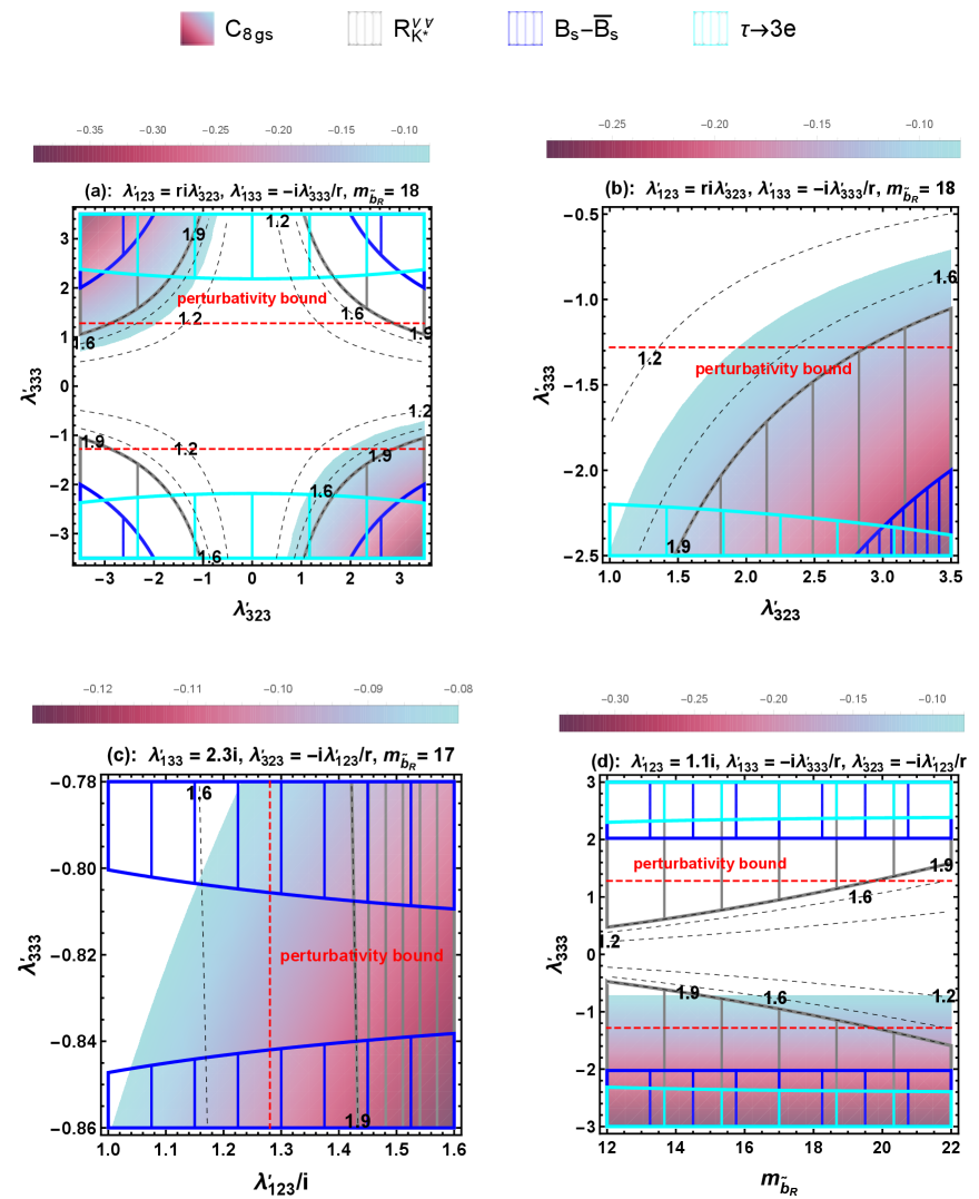
With the rough NP features above, next, we move onto the concrete numerical analysis. As shown in Fig. 2, ones can see that the Bd(s)K()K¯()B_{d(s)}\rightarrow K^{(\ast)}\bar{K}^{(\ast)} puzzle can be explained in RPV-MSSMIS, at 2σ2\sigma level. The τeee\tau\to eee decay, BsB¯sB_{s}-\bar{B}_{s} mixing, and BKνν¯B\rightarrow K^{\ast}\nu\bar{\nu} decay, provide the dominant constraints, and the perturbativity limit is also shown. In Fig. 2a, λ123\lambda^{\prime}_{123} and λ133\lambda^{\prime}_{133} are set related to λ323\lambda^{\prime}_{323} and λ333\lambda^{\prime}_{333}, respectively, and mb~Rm_{\tilde{b}_{R}} is 1818 TeV. The process-bound on λ333\lambda^{\prime}_{333} are mainly τeee\tau\to eee and BKνν¯B\rightarrow K^{\ast}\nu\bar{\nu} decays, while nearly overlapped by the exclusion area of perturbativity bound. With the same set, Fig. 2b shows the common region in detail, which shows that λ323\lambda^{\prime}_{323} should be larger than around 2.32.3 and λ333\lambda^{\prime}_{333} should be lower than around 0.7-0.7. In Fig. 2c, we set λ133=2.3i\lambda^{\prime}_{133}=2.3i, and then, the ranges for puzzle explanation are 1.02Im(λ123)1.291.02\lesssim{\rm Im}(\lambda^{\prime}_{123})\lesssim 1.29 and 0.84λ3330.8-0.84\lesssim\lambda^{\prime}_{333}\lesssim-0.8. In Fig. 2d, λ133\lambda^{\prime}_{133} is set as 1.1i1.1i, ones can see that the ratios RK()νν¯R^{\nu\bar{\nu}}_{K^{(\ast)}} increase with sbottom mass increasing for λ333>0\lambda^{\prime}_{333}>0, while decrease with sbottom mass increasing for λ333<0\lambda^{\prime}_{333}<0. The puzzle explanation favors 1.29λ3330.8-1.29\lesssim\lambda^{\prime}_{333}\lesssim-0.8 and mb~R15m_{\tilde{b}_{R}}\gtrsim 15 TeV.

mb~Rm_{\tilde{b}_{R}} λ123\lambda^{\prime}_{123} λ133\lambda^{\prime}_{133} λ323\lambda^{\prime}_{323} λ333\lambda^{\prime}_{333} RK()νν¯R^{\nu\bar{\nu}}_{K^{(\ast)}} C8gsNPC_{8gs}^{\rm NP} LKK¯L_{K\bar{K}} LKK¯L_{K^{\ast}\bar{K^{\ast}}} VP×105{\cal B}_{VP}\times 10^{5}
1717 TeV 1.2i1.2i 2.3i2.3i 3.323.32 0.81-0.81 1.641.64 0.084-0.084 23.5823.58 15.8015.80 0.800.80
1919 TeV 1.1i1.1i 2.8i2.8i 3.053.05 1-1 1.511.51 0.097-0.097 23.2323.23 15.2815.28 0.790.79
2121 TeV 1.1i1.1i 3.0i3.0i 3.053.05 1.07-1.07 1.391.39 0.104-0.104 23.0523.05 15.0115.01 0.790.79
Table 3: The benchmark points favored by the puzzle explanation. Here VP{\cal B}_{VP} is the untagged branching ratio (B¯sK0K¯0+c.c.){\cal B}(\bar{B}_{s}\rightarrow K^{\ast 0}\bar{K}^{0}+c.c.).

Afterwards, we collect some benchmark points in table 3 where the pseudoscalar-vector channel is also calculated. We consider the untagged transition B¯sK0K¯0\bar{B}_{s}\rightarrow K^{\ast 0}\bar{K}^{0} with the branching ratio measured as (B¯sK0K¯0+c.c.)exp=(1.98±0.28±0.50)×105{\cal B}(\bar{B}_{s}\rightarrow K^{\ast 0}\bar{K}^{0}+c.c.)_{\rm exp}=(1.98\pm 0.28\pm 0.50)\times 10^{-5} [67]. With the Wilson coefficient C8gsNP(μEW)C_{8gs}^{\rm NP}(\mu_{\rm EW}), ones can predict this branching ratio in NP [12],

(B¯sK0K¯0+c.c.)×105=0.87+0.87C8gsNP(μEW)+0.95C8gsNP(μEW)2.\displaystyle{\cal B}(\bar{B}_{s}\rightarrow K^{\ast 0}\bar{K}^{0}+c.c.)\times 10^{5}=0.87+0.87C_{8gs}^{\rm NP}(\mu_{\rm EW})+0.95C_{8gs}^{\rm NP}(\mu_{\rm EW})^{2}. (4.4)

5 Additional remarks

Before we conclude this work, it is worth making discussions on whether the imaginary λ\lambda^{\prime} couplings may affect CP violations. Firstly we check the NP CPV in the BsB¯sB_{s}-\bar{B}_{s} mixing. Given the formulas of Wilson coefficients shown in Eq. (3.3), along with flavor non-mixings in sneutrino content, the extra imaginary part , i.e. NP CPV not from CKM, can be only from the term, Λvv𝒩D2[mνv,mνv,mb~R,mb~R]\Lambda^{\prime\cal N}_{vv^{\prime}}D_{2}[m_{\nu_{v}},m_{\nu_{v^{\prime}}},m_{\tilde{b}_{R}},m_{\tilde{b}_{R}}], containing factor λ133λ323𝒱v()1𝒱v()3\lambda^{\prime}_{133}\lambda^{\prime\ast}_{323}{\cal V}_{v^{(\prime)}1}{\cal V}^{\ast}_{v^{(\prime)}3}. However, 𝒱v()1𝒱v()3{\cal V}_{v^{(\prime)}1}{\cal V}^{\ast}_{v^{(\prime)}3} for light-neutrino content provides suppressing effects due to the unitarity of PMNS. In concrete numerical calculations, we confirm that this imaginary contribution can be omitted.

Next we examine the potential CPV from ZZ boson partical decay, which are proportional to ratios of the coupling constants, Im(λiJ3λiJ3/λ1J3λ1J3){\rm Im}\left({\lambda^{\prime\ast}_{iJ3}\lambda^{\prime}_{iJ^{\prime}3}}/{\lambda^{\prime\ast}_{1J3}\lambda^{\prime}_{1J^{\prime}3}}\right) [68]. Given we set λ123\lambda^{\prime}_{123} and λ133\lambda^{\prime}_{133} both purely imaginary, while λ323\lambda^{\prime}_{323} and λ333\lambda^{\prime}_{333} both real, these ratios have no imaginary part.

At last, we move onto the electron electric dipole moment (EDM), that is proportional to the factor [(cos2βλ1jksin2βλ1jk)sinαAd+cosβλ1jksinβλ1jkcosαAd)]|λ1jk|2[(\cos^{2}\beta_{\lambda^{\prime}_{1jk}}-\sin^{2}\beta_{\lambda^{\prime}_{1jk}})\sin\alpha_{A_{d}}+\cos\beta_{\lambda^{\prime}_{1jk}}\sin\beta_{\lambda^{\prime}_{1jk}}\cos\alpha_{A_{d}})]|\lambda^{\prime}_{1jk}|^{2} [69], where the αAd\alpha_{A_{d}} and βλ1jk\beta_{\lambda^{\prime}_{1jk}} are the related arguments. In the scenario of this work, we have βλ1jk=π/2\beta_{\lambda^{\prime}_{1jk}}=\pi/2. With a suppressed non-positive αAd\alpha_{A_{d}}, the EDM constraint can be fulfilled.

6 Conclusions

The recent measurements of Bd(s)K()K¯()B_{d(s)}\rightarrow K^{(\ast)}\bar{K}^{(\ast)} show a non-leptonic puzzle, which expresses the deviations between the data and the QCD-factorisation prediction for the U-spin related observable, LK()K()¯L_{K^{(\ast)}\bar{K^{(\ast)}}}. Besides, Belle II has recently reported the new measurement of (B+K+νν¯){\cal B}(B^{+}\rightarrow K^{+}\nu\bar{\nu}), around 2.7σ2.7\sigma above the SM prediction. Both of the tensions imply that, there may exist new quark-flavor structure beyond the SM.

In this work, we study the non-leptonic puzzle and B+K+νν¯B^{+}\rightarrow K^{+}\nu\bar{\nu} in RPV-MSSMIS. This NP framework connects the trilinear interaction λL^Q^D^\lambda^{\prime}\hat{L}\hat{Q}\hat{D} with the (s)neutrino chirality flip to make the unique contribution to LK()K()¯L_{K^{(\ast)}\bar{K^{(\ast)}}}, through the gluon-penguin diagrams. The chiral-flip effects are expressed as the double-λ\lambda^{\prime} terms in the Wilson coefficient C8gs,dNPC^{\rm NP}_{8gs,d}, which can be enhanced by the logarithm and make the related deviation explained. In the BsB¯sB_{s}-\bar{B}_{s} mixing, there also exist chiral-flip contributions, and to fulfill the strict bound of experimental data, the scenario of imaginary λ123\lambda^{\prime}_{123}, λ133\lambda^{\prime}_{133} with real λ323\lambda^{\prime}_{323}, λ333\lambda^{\prime}_{333} is adopted. The effect on the CPV due to this scenario is investigated as well. As for B+K+νν¯B^{+}\rightarrow K^{+}\nu\bar{\nu} decays, we find that the large |λ133||\lambda^{\prime}_{133}| and |λ323||\lambda^{\prime}_{323}|, can make some enhancements, even when sbottoms are as heavy as 1010 TeV. At last, we provide some benchmark points, which also fulfill collider bounds, neutrino data, and series of flavor-physics constraints from BB,KK-semileptonic decays, ZZ-pole data, cLFV processes, etc.

Acknowledgements

M.D. thanks Xing-Bo Yuan for valuable discussions. This work is supported in part by the National Natural Science Foundation of China under Grant No. 12275367, the Fundamental Research Funds for the Central Universities, and the Sun Yat-Sen University Science Foundation.

Appendix A The numerical form of the (s)neutrino mixing matrix

With the input set in table 2, the numerical form of the neutrino mixing matrix is listed as

𝒱T(0.8360.5260.1450.034i000.034000.2460.6000.76100.013i000.01300.4880.6020.632000.012i000.0120000.707i000.7070000000.707i000.7070000000.707i000.7070.0410.0260.0070.706i000.706000.0050.0110.01500.707i000.70700.0080.0100.011000.707i000.707),\displaystyle{\cal V}^{T}\approx\left(\begin{array}[]{ccccccccc}0.836&0.526&-0.145&0.034i&0&0&-0.034&0&0\\ -0.246&0.600&0.761&0&0.013i&0&0&0.013&0\\ 0.488&-0.602&0.632&0&0&0.012i&0&0&0.012\\ 0&0&0&-0.707i&0&0&-0.707&0&0\\ 0&0&0&0&-0.707i&0&0&0.707&0\\ 0&0&0&0&0&-0.707i&0&0&0.707\\ -0.041&-0.026&0.007&0.706i&0&0&-0.706&0&0\\ 0.005&-0.011&-0.015&0&0.707i&0&0&0.707&0\\ -0.008&0.010&-0.011&0&0&0.707i&0&0&0.707\\ \end{array}\right), (A.10)

which is related to the neutrino mass spectrum around {0,8×1015,5×1014,1,1,1,1,1,1}\{0,8\times 10^{-15},5\times 10^{-14},1,1,1,1,1,1\} TeV. And the sneutrino mixing matrices are given numerically by

𝒱~(0.045000.473000.8800000.018000.475000.8800000.016000.475000.8800.995000.102000.0040000.999000.0380000000.999000.0350000.091000.875000.4750000.034000.880000.4750000.030000.880000.475),\displaystyle{\cal\tilde{V}}^{\cal R}\approx\left(\begin{array}[]{ccccccccc}-0.045&0&0&-0.473&0&0&0.880&0&0\\ 0&-0.018&0&0&-0.475&0&0&0.880&0\\ 0&0&-0.016&0&0&-0.475&0&0&0.880\\ 0.995&0&0&-0.102&0&0&-0.004&0&0\\ 0&0.999&0&0&-0.038&0&0&0&0\\ 0&0&-0.999&0&0&0.035&0&0&0\\ -0.091&0&0&-0.875&0&0&-0.475&0&0\\ 0&-0.034&0&0&-0.880&0&0&-0.475&0\\ 0&0&-0.030&0&0&-0.880&0&0&-0.475\\ \end{array}\right), (A.20)

related to the mν~m_{\tilde{\nu}^{\cal R}} spectrum {269,272,272,1010,1000,1000,1129,1127,1127}\{269,272,272,1010,1000,1000,1129,1127,1127\} GeV, as well as

𝒱~(0.080000.875000.4770000.034000.879000.4750000.031000.880000.4750.996000.093000.0030000.999000.0380000000.999000.0350000.047000.474000.8790000.018000.475000.8800000.016000.475000.880),\displaystyle{\cal\tilde{V}}^{\cal I}\approx\left(\begin{array}[]{ccccccccc}0.080&0&0&0.875&0&0&-0.477&0&0\\ 0&-0.034&0&0&-0.879&0&0&0.475&0\\ 0&0&-0.031&0&0&-0.880&0&0&0.475\\ -0.996&0&0&0.093&0&0&0.003&0&0\\ 0&-0.999&0&0&0.038&0&0&0&0\\ 0&0&-0.999&0&0&0.035&0&0&0\\ -0.047&0&0&-0.474&0&0&-0.879&0&0\\ 0&0.018&0&0&0.475&0&0&0.880&0\\ 0&0&0.016&0&0&0.475&0&0&0.880\\ \end{array}\right), (A.30)

related to the mν~m_{\tilde{\nu}^{\cal I}} spectrum {854,854,854,1010,1000,1000,1389,1388,1388}\{854,854,854,1010,1000,1000,1389,1388,1388\} GeV.

Then ones can find, all the chargino-sneutrino diagrams and the neutralino-slepton diagrams, among the non-λ\lambda^{\prime} diagrams in the cLFV decays of leptons, make negligible contributions due to the vanishing of flavor mixing in sneutrino sector, as shown in Eq. (A.20) and Eq. (A.30). As to W/H±W/H^{\pm}-neutrino diagrams, they are always connected to terms 𝒱(α+3)vT𝒱(β+3)vT{\cal V}^{T\ast}_{(\alpha+3)v}{\cal V}^{T}_{(\beta+3)v}, 𝒱(α+3)vT𝒱βvT{\cal V}^{T\ast}_{(\alpha+3)v}{\cal V}^{T}_{\beta v}, 𝒱αvT𝒱βvT{\cal V}^{T\ast}_{\alpha v}{\cal V}^{T}_{\beta v} and conjugate terms (α,β=e,μ,τ\alpha,\beta=e,\mu,\tau and αβ\alpha\neq\beta). Readers can see calculations of these diagrams in Ref. [70]. With the numerical form of Eq. (A.10), the 𝒱(α+3)vT𝒱(β+3)vT{\cal V}^{T\ast}_{(\alpha+3)v}{\cal V}^{T}_{(\beta+3)v} and 𝒱(α+3)vT𝒱βvT{\cal V}^{T\ast}_{(\alpha+3)v}{\cal V}^{T}_{\beta v} terms vanish. The 𝒱αvT𝒱βvT{\cal V}^{T\ast}_{\alpha v}{\cal V}^{T}_{\beta v} term can be decomposed into two parts, N=49𝒱αNT𝒱βNT\sum_{N=4}^{9}{\cal V}^{T\ast}_{\alpha N}{\cal V}^{T}_{\beta N} and i=13𝒱αiT𝒱βiT=N=49𝒱αNT𝒱βNT\sum_{i=1}^{3}{\cal V}^{T\ast}_{\alpha i}{\cal V}^{T}_{\beta i}=-\sum_{N=4}^{9}{\cal V}^{T\ast}_{\alpha N}{\cal V}^{T}_{\beta N}, related to the nearly degenerate heavy neutrinos and light neutrinos respectively [71]. Then ones can also find that the 𝒱αvT𝒱βvT{\cal V}^{T\ast}_{\alpha v}{\cal V}^{T}_{\beta v} term makes no effective contribution to the cLFV decays. Thus, we conclude that the non-λ\lambda^{\prime} diagrams provide negligible effects on the cLFV decays, as mentioned in section 3.3, in our input sets.

References

  • [1] LHCb Collaboration, R. Aaij et al., Test of lepton universality in bs+b\rightarrow s\ell^{+}\ell^{-} decays, Phys. Rev. Lett. 131 (2023), no. 5 051803, [arXiv:2212.09152].
  • [2] A. Biswas, S. Descotes-Genon, J. Matias, and G. Tetlalmatzi-Xolocotzi, A new puzzle in non-leptonic B decays, JHEP 06 (2023) 108, [arXiv:2301.10542].
  • [3] Particle Data Group Collaboration, R. L. Workman et al., Review of Particle Physics, PTEP 2022 (2022) 083C01.
  • [4] BaBar Collaboration, B. Aubert et al., Observation of B0B^{0}\to K*0 K¯\bar{K}* 0 and search for B0B^{0}\to K*0 K*0, Phys. Rev. Lett. 100 (2008) 081801, [arXiv:0708.2248].
  • [5] LHCb Collaboration, R. Aaij et al., Amplitude analysis of the B(s)0K0K¯0B^{0}_{(s)}\to K^{*0}\overline{K}^{*0} decays and measurement of the branching fraction of the B0K0K¯0B^{0}\to K^{*0}\overline{K}^{*0} decay, JHEP 07 (2019) 032, [arXiv:1905.06662].
  • [6] BaBar Collaboration, B. Aubert et al., Observation of B+K¯0K+B^{+}\to\bar{K}^{0}K^{+} and B0K0K¯0B^{0}\to K^{0}\bar{K}^{0}, Phys. Rev. Lett. 97 (2006) 171805, [hep-ex/0608036].
  • [7] Belle Collaboration, Y. T. Duh et al., Measurements of branching fractions and direct CP asymmetries for BKπB\to K\pi, BππB\to\pi\pi and BKKB\to KK decays, Phys. Rev. D 87 (2013), no. 3 031103, [arXiv:1210.1348].
  • [8] Belle Collaboration, B. Pal et al., Observation of the decay Bs0K0K¯0B_{s}^{0}\rightarrow K^{0}\overline{K}^{0}, Phys. Rev. Lett. 116 (2016), no. 16 161801, [arXiv:1512.02145].
  • [9] LHCb Collaboration, R. Aaij et al., Measurement of the branching fraction of the decay Bs0KS0KS0B_{s}^{0}\to K_{S}^{0}K_{S}^{0}, Phys. Rev. D 102 (2020), no. 1 012011, [arXiv:2002.08229].
  • [10] M. Beneke, G. Buchalla, M. Neubert, and C. T. Sachrajda, QCD factorization in B —>> pi K, pi pi decays and extraction of Wolfenstein parameters, Nucl. Phys. B 606 (2001) 245–321, [hep-ph/0104110].
  • [11] M. Algueró, A. Crivellin, S. Descotes-Genon, J. Matias, and M. Novoa-Brunet, A new BB-flavour anomaly in Bd,sK0K¯0B_{d,s}\to K^{*0}\bar{K}^{*0}: anatomy and interpretation, JHEP 04 (2021) 066, [arXiv:2011.07867].
  • [12] A. Biswas, S. Descotes-Genon, J. Matias, and G. Tetlalmatzi-Xolocotzi, Optimised observables and new physics prospects in the penguin-mediated decays Bd(s)K()0ϕB_{d(s)}\rightarrow K^{(\ast)0}\phi, JHEP 08 (2024) 030, [arXiv:2404.01186].
  • [13] J. M. Lizana, J. Matias, and B. A. Stefanek, Explaining the Bd,sK()K¯(){B}_{d,s}\to{K}^{\left(\ast\right)}{\overline{K}}^{\left(\ast\right)} non-leptonic puzzle and charged-current B-anomalies via scalar leptoquarks, JHEP 09 (2023) 114, [arXiv:2306.09178].
  • [14] M.-D. Zheng and H.-H. Zhang, Studying the bs+b\rightarrow s\ell^{+}\ell^{-} anomalies and (g2)μ(g-2)_{\mu} in RR-parity violating MSSM framework with the inverse seesaw mechanism, Phys. Rev. D 104 (2021), no. 11 115023, [arXiv:2105.06954].
  • [15] M.-D. Zheng, F.-Z. Chen, and H.-H. Zhang, Explaining anomalies of B-physics, muon g2g-2 and W mass in R-parity violating MSSM with seesaw mechanism, Eur. Phys. J. C 82 (2022), no. 10 895, [arXiv:2207.07636].
  • [16] Belle-II Collaboration, I. Adachi et al., Evidence for B+K+ννB+\rightarrow K+\nu\nu decays, Phys. Rev. D 109 (2024), no. 11 112006, [arXiv:2311.14647].
  • [17] D. Bečirević, G. Piazza, and O. Sumensari, Revisiting BK()νν¯B\rightarrow K^{(*)}\nu{\bar{\nu}} decays in the Standard Model and beyond, Eur. Phys. J. C 83 (2023), no. 3 252, [arXiv:2301.06990].
  • [18] J. Rosiek, Complete Set of Feynman Rules for the Minimal Supersymmetric Extension of the Standard Model, Phys. Rev. D 41 (1990) 3464.
  • [19] J. Rosiek, Complete set of Feynman rules for the MSSM: Erratum, hep-ph/9511250.
  • [20] V. De Romeri, K. M. Patel, and J. W. Valle, Inverse seesaw mechanism with compact supersymmetry: Enhanced naturalness and light superpartners, Phys. Rev. D 98 (2018), no. 7 075014, [arXiv:1808.01453].
  • [21] H. An, P. S. B. Dev, Y. Cai, and R. N. Mohapatra, Sneutrino Dark Matter in Gauged Inverse Seesaw Models for Neutrinos, Phys. Rev. Lett. 108 (2012) 081806, [arXiv:1110.1366].
  • [22] T. Besmer and A. Steffen, R-parity violation and the decay b —>> s gamma, Phys. Rev. D 63 (2001) 055007, [hep-ph/0004067].
  • [23] A. J. Buras, J. Girrbach-Noe, C. Niehoff, and D. M. Straub, BK()νν¯B\to{K}^{\left(\ast\right)}\nu\overline{\nu} decays in the Standard Model and beyond, JHEP 02 (2015) 184, [arXiv:1409.4557].
  • [24] C. S. Kim, D. Sahoo, and K. N. Vishnudath, Searching for signatures of new physics in BKνν¯B\rightarrow K\,\nu\,\overline{\nu} to distinguish between Dirac and Majorana neutrinos, Eur. Phys. J. C 84 (2024), no. 9 882, [arXiv:2405.17341].
  • [25] X.-G. He, X.-D. Ma, and G. Valencia, Revisiting models that enhance B+K+νν¯B^{+}\rightarrow K^{+}\nu\bar{\nu} in light of the new Belle II measurement, Phys. Rev. D 109 (2024), no. 7 075019, [arXiv:2309.12741].
  • [26] Belle Collaboration, J. Grygier et al., Search for 𝐁𝐡𝛎𝛎¯\boldsymbol{B\to h\nu\bar{\nu}} decays with semileptonic tagging at Belle, Phys. Rev. D 96 (2017), no. 9 091101, [arXiv:1702.03224]. [Addendum: Phys.Rev.D 97, 099902 (2018)].
  • [27] B.-F. Hou, X.-Q. Li, M. Shen, Y.-D. Yang, and X.-B. Yuan, Deciphering the Belle II data on BKνν¯B\to K\nu\overline{\nu} decay in the (dark) SMEFT with minimal flavour violation, JHEP 06 (2024) 172, [arXiv:2402.19208].
  • [28] F.-Z. Chen, Q. Wen, and F. Xu, Correlating BK()νν¯B\rightarrow K^{(*)}\nu\bar{\nu} and flavor anomalies in SMEFT, Eur. Phys. J. C 84 (2024), no. 10 1012, [arXiv:2401.11552].
  • [29] ATLAS Collaboration, M. Aaboud et al., Search for B-L R -parity-violating top squarks in s\sqrt{s} =13 TeV pp collisions with the ATLAS experiment, Phys. Rev. D 97 (2018), no. 3 032003, [arXiv:1710.05544].
  • [30] CMS Collaboration, A. M. Sirunyan et al., Search for long-lived particles decaying into displaced jets in proton-proton collisions at s=\sqrt{s}= 13 TeV, Phys. Rev. D 99 (2019), no. 3 032011, [arXiv:1811.07991].
  • [31] ATLAS Collaboration, M. Aaboud et al., Search for heavy charged long-lived particles in the ATLAS detector in 36.1 fb-1 of proton-proton collision data at s=13\sqrt{s}=13 TeV, Phys. Rev. D 99 (2019), no. 9 092007, [arXiv:1902.01636].
  • [32] ATLAS Collaboration, G. Aad et al., Search for long-lived, massive particles in events with a displaced vertex and a muon with large impact parameter in pppp collisions at s=13\sqrt{s}=13 TeV with the ATLAS detector, Phys. Rev. D 102 (2020), no. 3 032006, [arXiv:2003.11956].
  • [33] ATLAS Collaboration, G. Aad et al., Search for R-parity-violating supersymmetry in a final state containing leptons and many jets with the ATLAS experiment using s=13TeV\sqrt{s}=13{TeV} proton–proton collision data, Eur. Phys. J. C 81 (2021), no. 11 1023, [arXiv:2106.09609].
  • [34] CMS Collaboration, A. M. Sirunyan et al., Search for top squark production in fully-hadronic final states in proton-proton collisions at s=\sqrt{s}= 13 TeV, Phys. Rev. D 104 (2021), no. 5 052001, [arXiv:2103.01290].
  • [35] CMS Collaboration, A. Tumasyan et al., Combined searches for the production of supersymmetric top quark partners in proton–proton collisions at s=13TeV\sqrt{s}=13\,\text{Te}\text{V}, Eur. Phys. J. C 81 (2021), no. 11 970, [arXiv:2107.10892].
  • [36] ATLAS Collaboration, M. Aaboud et al., Search for supersymmetry in events with four or more leptons in s=13\sqrt{s}=13 TeV pppp collisions with ATLAS, Phys. Rev. D 98 (2018), no. 3 032009, [arXiv:1804.03602].
  • [37] ATLAS Collaboration, M. Aaboud et al., Search for lepton-flavor violation in different-flavor, high-mass final states in pppp collisions at s=13\sqrt{s}=13 TeV with the ATLAS detector, Phys. Rev. D 98 (2018), no. 9 092008, [arXiv:1807.06573].
  • [38] ATLAS Collaboration, G. Aad et al., Search for supersymmetry in events with four or more charged leptons in 139fb-1139\,\mbox{fb${}^{-1}$} of s=13\sqrt{s}=13 TeV pppp collisions with the ATLAS detector, JHEP 07 (2021) 167, [arXiv:2103.11684].
  • [39] ATLAS Collaboration, G. Aad et al., Search for heavy Higgs bosons with flavour-violating couplings in multi-lepton plus b-jets final states in pp collisions at 13 TeV with the ATLAS detector, JHEP 12 (2023) 081, [arXiv:2307.14759].
  • [40] Particle Data Group Collaboration, S. Navas et al., Review of particle physics, Phys. Rev. D 110 (2024), no. 3 030001.
  • [41] J. Aebischer, J. Kumar, P. Stangl, and D. M. Straub, A Global Likelihood for Precision Constraints and Flavour Anomalies, Eur. Phys. J. C 79 (2019), no. 6 509, [arXiv:1810.07698].
  • [42] K. Earl and T. Grégoire, Contributions to bsb\rightarrow s\ell\ell Anomalies from RR-Parity Violating Interactions, JHEP 08 (2018) 201, [arXiv:1806.01343].
  • [43] Q.-Y. Hu, Y.-D. Yang, and M.-D. Zheng, Revisiting the BB-physics anomalies in RR-parity violating MSSM, Eur. Phys. J. C 80 (2020), no. 5 365, [arXiv:2002.09875].
  • [44] D. Bryman, V. Cirigliano, A. Crivellin, and G. Inguglia, Testing Lepton Flavor Universality with Pion, Kaon, Tau, and Beta Decays, arXiv:2111.05338.
  • [45] A. M. Coutinho, A. Crivellin, and C. A. Manzari, Global Fit to Modified Neutrino Couplings and the Cabibbo-Angle Anomaly, Phys. Rev. Lett. 125 (2020), no. 7 071802, [arXiv:1912.08823].
  • [46] M. Blennow, P. Coloma, E. Fernández-Martínez, and M. González-López, Right-handed neutrinos and the CDF II anomaly, Phys. Rev. D 106 (2022), no. 7 073005, [arXiv:2204.04559].
  • [47] LHCb Collaboration, R. Aaij et al., Search for the rare decay D0μ+μD^{0}\to\mu^{+}\mu^{-}, Phys. Lett. B 725 (2013) 15–24, [arXiv:1305.5059].
  • [48] LHCb Collaboration, R. Aaij et al., Search for Rare Decays of D0 Mesons into Two Muons, Phys. Rev. Lett. 131 (2023), no. 4 041804, [arXiv:2212.11203].
  • [49] Belle Collaboration, N. Tsuzuki et al., Search for lepton-flavor-violating τ\tau decays into a lepton and a vector meson using the full Belle data sample, JHEP 06 (2023) 118, [arXiv:2301.03768].
  • [50] S. Nandi, S. K. Patra, and A. Soni, Correlating new physics signals in BD()τντB\to D^{(*)}\tau\nu_{\tau} with BτντB\to\tau\nu_{\tau}, arXiv:1605.07191.
  • [51] Q.-Y. Hu, X.-Q. Li, Y. Muramatsu, and Y.-D. Yang, R-parity violating solutions to the RD()R_{D^{(\ast)}} anomaly and their GUT-scale unifications, Phys. Rev. D99 (2019), no. 1 015008, [arXiv:1808.01419].
  • [52] G. Passarino and M. J. G. Veltman, One Loop Corrections for e+ e- Annihilation Into mu+ mu- in the Weinberg Model, Nucl. Phys. B160 (1979) 151–207.
  • [53] A. Denner, Techniques for calculation of electroweak radiative corrections at the one loop level and results for W physics at LEP-200, Fortsch. Phys. 41 (1993) 307–420, [arXiv:0709.1075].
  • [54] R. J. Dowdall, C. T. H. Davies, R. R. Horgan, G. P. Lepage, C. J. Monahan, J. Shigemitsu, and M. Wingate, Neutral B-meson mixing from full lattice QCD at the physical point, Phys. Rev. D 100 (2019), no. 9 094508, [arXiv:1907.01025].
  • [55] J. T. Tsang and M. Della Morte, B-physics from lattice gauge theory, Eur. Phys. J. ST 233 (2024), no. 2 253–270, [arXiv:2310.02705].
  • [56] HFLAV Collaboration, Y. S. Amhis et al., Averages of b-hadron, c-hadron, and τ\tau-lepton properties as of 2021, Phys. Rev. D 107 (2023), no. 5 052008, [arXiv:2206.07501].
  • [57] J. Albrecht, F. Bernlochner, A. Lenz, and A. Rusov, Lifetimes of b-hadrons and mixing of neutral B-mesons: theoretical and experimental status, Eur. Phys. J. ST 233 (2024), no. 2 359–390, [arXiv:2402.04224].
  • [58] A. de Gouvea, S. Lola, and K. Tobe, Lepton flavor violation in supersymmetric models with trilinear R-parity violation, Phys. Rev. D63 (2001) 035004, [hep-ph/0008085].
  • [59] D. Buttazzo, A. Greljo, G. Isidori, and D. Marzocca, B-physics anomalies: a guide to combined explanations, JHEP 11 (2017) 044, [arXiv:1706.07808].
  • [60] M. Misiak, A. Rehman, and M. Steinhauser, Towards B¯Xsγ\overline{B}\to{X}_{s}\gamma at the NNLO in QCD without interpolation in mc, JHEP 06 (2020) 175, [arXiv:2002.01548].
  • [61] HFLAV Collaboration, Y. S. Amhis et al., Averages of b-hadron, c-hadron, and τ\tau-lepton properties as of 2018, Eur. Phys. J. C 81 (2021), no. 3 226, [arXiv:1909.12524].
  • [62] P. Arnan, D. Becirevic, F. Mescia, and O. Sumensari, Probing low energy scalar leptoquarks by the leptonic WW and ZZ couplings, JHEP 02 (2019) 109, [arXiv:1901.06315].
  • [63] ALEPH, DELPHI, L3, OPAL, SLD, LEP Electroweak Working Group, SLD Electroweak Group, SLD Heavy Flavour Group Collaboration, S. Schael et al., Precision electroweak measurements on the ZZ resonance, Phys. Rept. 427 (2006) 257–454, [hep-ex/0509008].
  • [64] M.-D. Zheng, F.-Z. Chen, and H.-H. Zhang, The WνW\ell\nu-vertex corrections to W-boson mass in the R-parity violating MSSM, AAPPS Bull. 33 (2023), no. 1 16, [arXiv:2204.06541].
  • [65] I. Esteban, M. Gonzalez-Garcia, M. Maltoni, T. Schwetz, and A. Zhou, The fate of hints: updated global analysis of three-flavor neutrino oscillations, JHEP 09 (2020) 178, [arXiv:2007.14792].
  • [66] J. S. Alvarado and R. Martinez, PMNS matrix in a non-universal U(1)XU(1)_{X} extension to the MSSM with one massless neutrino, arXiv:2007.14519.
  • [67] LHCb Collaboration, R. Aaij et al., Amplitude analysis of Bs0KS0K±πB^{0}_{s}\rightarrow K^{0}_{S}K^{\pm}\pi^{\mp} decays, JHEP 06 (2019) 114, [arXiv:1902.07955].
  • [68] R. Barbier et al., R-parity violating supersymmetry, Phys. Rept. 420 (2005) 1–202, [hep-ph/0406039].
  • [69] R. Adhikari and G. Omanovic, LSND, solar and atmospheric neutrino oscillation experiments, and R-parity violating supersymmetry, Phys. Rev. D 59 (1999) 073003.
  • [70] A. Abada, M. E. Krauss, W. Porod, F. Staub, A. Vicente, and C. Weiland, Lepton flavor violation in low-scale seesaw models: SUSY and non-SUSY contributions, JHEP 11 (2014) 048, [arXiv:1408.0138].
  • [71] J. Chang, K. Cheung, H. Ishida, C.-T. Lu, M. Spinrath, and Y.-L. S. Tsai, A supersymmetric electroweak scale seesaw model, JHEP 10 (2017) 039, [arXiv:1707.04374].