[figure]style=plain,subcapbesideposition=top
Experimental violation of the Leggett-Garg inequality with a single-spin system
Abstract
Investigation the boundary between quantum mechanical description and classical realistic view is of fundamental importance. The Leggett-Garg inequality provides a criterion to distinguish between quantum systems and classical systems, and can be used to prove the macroscopic superposition state. A larger upper bound of the LG function can be obtained in a multi-level system. Here, we present an experimental violation of the Leggett-Garg inequality in a three-level system using nitrogen-vacancy center in diamond by ideal negative result measurement. The experimental maximum value of Leggett-Garg function is which exceeds the Lders bound with a level of confidence.
The objects we can see with our naked eye are composed of a very large number of atoms, and these atoms can be in a quantum superposition state. If the laws of quantum mechanics are extrapolating to the laws satisfied by everyday objects, there is inevitably the prospect of macroscopic coherence. Schrdinger’s cat, simultaneously both dead and alive, is considered to be one of the most characteristic examples of macroscopic coherence. This situation runs counter to our intuitive understanding of how the daily macroworld works.
Leggett and Garg gave a method to verify whether a given system can be in a superposition of discrete statesLeggett_1985 . They proposed two assumptions that the classical world certainly satisfiedLeggett_2002 ; Leggett_2008 : (i) macroscopic realism (MR)— that a system cannot be in a superposition of the classically observable state and the measurement of the object will get a certain value; (ii) Non-invasive measurability (NIM)—that it is possible in principle to determine the state of a system with arbitrarily precision without destroying its subsequent evolution. Classical world meet the requirements of these assumptions, but for quantum mechanics, neither of these two assumptions can be satisfied. The Leggett-Garg inequality (LGI) is a test of MR under a set of reasonable assumptions about the system, in particular a version of NIM. The violation of the inequality leads to the conclusion that either MR or the other assumptions is wrongMaroney_2014 . In this way, the LGI provide a method to investigate the existence of macroscopic coherence and to test the applicability of quantum mechanics as we scale from microscopic to macroscopic worldLeggett_2002 .
Until recently it has been believed that the maximal violation of three-time measurement LGI, which characterized the correlation between the results of this measurements, is independent of the number of possible macroscopically distinct states of the system. This is due to the fact that the measurements are dichotomicKatiyar_2017 . However, Budroni and EmaryBudroni_2014 showed that this is only true if the measurement follows the naive Lders update ruleluder_1951 . According to Lders rule, the state is updated as depending on the outcome of the measurement, where and are two projectors on eigenspaces associated with measurement results and . In a more general case, one can observe greater violations by using a higher-dimensional system. Therefore, striving for a larger violation value in a higher-dimensional system is worth studying. The quantum upper bound of the LGI depends on both the details of the measurement and the dimension of the systemKatiyar_2017 . For the LGI experiment performed on the three-level system, a higher theoretical quantum upper bound can be obtained than that on the two-level systemPalacios-Laloy_2010 ; Katiyar_2013 ; Dressel_2011 . With interest in the beyond quantum upper bound of the LGI, the NMR systemKatiyar_2017 and single photonWang_2017 are used to mimic the three-level system. There is also a work performed in a single three-level systemGeorge_2013 . However, this work used the projective measurement which is invasive measurement method and fails to convince a macrorealist. Achieving the violation of the LGI which breaks through the Lders bound in a single three-level system remains elusive. Here, we report an experimental violation of LGI with the exceeding of Lders bound in a real three-level system. Our experiment is performed in a single nitrogen-vacancy (NV) center in diamond. The Ideal Negative Result Measurement (INRM) method is implemented to avoid invasive measurementsKatiyar_2017 ; Knee_2012 .
The LGI test the correlations of a single system measured at different times. The most frequently encountered inequalities concern the n-measurement LG stringsBudroni_2014
| (1) |
Here, is a macroscopic dichotomic variable with distinct outcomes , at some time , the outcomes of these measurements are denoted as and , denotes the number of time steps. In a macrorealistic system, the outcomes represent the two distinct sates of the system. The correlation function is , where is the joint probability to obtain and at times and . The n-measurement LGIs are bounded as follows. If and odd then , and if and even then Budroni_2014 . In the typical three-time measurement LGI scenario as shown in Fig. 1(a), the LG function is given byEmary_2014
| (2) |
More specifically, when the measurements performed to the system do not disturb the system (NIM assumption) and the system is classical (macrorealistic), the value of is bounded by . On the other hand, when the system is quantum, it is possible to choose the evolution time between measurements in such a way that will go beyond 1, violating the LGI that Emary_2014 . Quantum mechanical experiments are able to violate three-time measurement LGI up to 1.5 for a qubit with dichotomic measurements . More general systems have the same bound when the measurements follow the Lders update rule. However, if one relaxes the assumption that the measurement follows the Lders update rule, the quantum bound on could be extended to a value that depends on the dimension of the systemBudroni_2014 . For a three-level system, the measurement operators are , and corresponding to the three states of system. and are associated with outcome . is associated with outcome . The quantum state after the measurement is updated as or depending on whether the measurement result is or . This protocol is different from the Lders rule and can lead to the value in the ideal case.

Ideal negative result measurement is one of candidates to achieve non-invasive measurement. Measurement process can be regarded as an interaction process between the system to be measured and the apparatus. For instance, a detector couples with one of system states, registering a ‘click’ if the system is in the specific state, but it does not interact with the other states. If the detector clicks, the result is discarded, and if it does not click, we keep the result. In this way, we can infer system states without any interaction between the system to be measured and the apparatus by keeping only the negative (no click) results. In our scheme, the INRM scheme is realized by controlled gates and the postselection of the ancilla qubit state as depicted in Fig. 1(b). The ancillary qubit is initialized in the state . The controlled gates flip the ancilla qubit except when the three-level system is in one of the three states. Postselecting the situation that the ancilla qubit has not been flipped, the non-invasiveness of the measurement can be guaranteed.
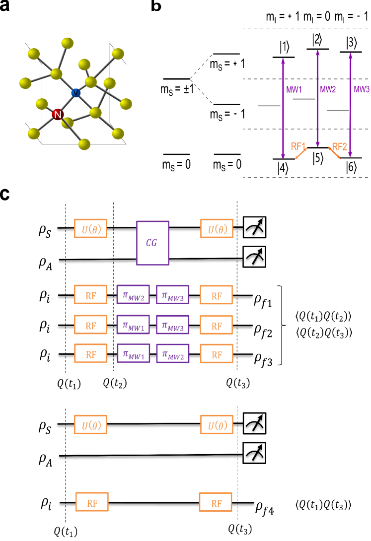
Our experiment was implemented on an NV center in diamond. As depicted in Fig. 2(a), the NV center consists of a substitutional nitrogen atom with an adjacent vacancy site in the diamond crystal lattice. The three energy levels of 14N nuclear spin, , and , make up the three-level system. Two NV electron spin energy levels, and , are chosen as an ancilla qubit. The Hamiltonian of the NV center is Wu_2018 , where and are corresponding spin operators of the electron and nuclear spin, is the zero-field splitting of electron spin, is the nuclear quadrupolar interaction, and is the hyperfine interaction. The experiment is performed on an optically detected magnetic resonance setup. A magnetic field of 512 G is applied along the NV symmetry axis ([111] crystal axis), yielding Zeeman frequencies and . The total system utilized in our experiment is spanned by six energy levels, consisting of , , , , and , relabeled by , , , , and as depicted in Fig. 2(b).
The INRM is performed by the selective microwave pulses and postselecting the populations of the final states. The two microwave pulses, as shown in Fig. 2(c), realize the controlled gate which flips the ancilla qubit when the system in two of the three states (see Appendix A for detailed discussion). The three experiments correspond to the situation where the system is in three different states to ensure that the ancilla qubit is not flipped. The transition frequency of the microwave pulses is about 4.303 GHz, which is much different from the nuclear spin transition frequency on the megahertz order. These microwave pulses hardly flip the state of the nuclear spin. The non-invasiveness of the measurement is ensured by the postselecting the populations of the final states which indicate the case that the ancilla qubit is not flipped. The NV center is initialized to the state via laser pulsesJacques_2009 . The postselection procedure is implemented by preserving the population of , and in the final states. Although the pulses in experiments will cause unwanted transitions due to finite off-resonance, these transitions can be removed through the postselection procedure. To verify the LG inequality, two time correlations of the measurements, , need to be obtained. Regarding the initialization as the first measurement, thus , the tested LG inequality is reduced to + – . The value of can be obtained from joint probability of measurement outcomes when the controlled gates are performed. The value can be obtained from directly measurement without controlled gates intersected. The relationships between three terms in LG function and final state populations are shown below (see Appendix B for detailed calculations):
| (8) |
where denotes the population of ith energy level of the final state in Fig. 2(c), where .
The evolution of the rotation on the three-level system is , where and is spin operator of spin-1 system. The operation can be realized in rotating frame by applying two radio frequency pulses simultaneously on the nuclear spin. The frequencies of the two pulses are , the resonance frequency between level and , and , the resonance frequency between level and . is the Rabi frequency which is proportional to strength of radio frequency pulses, which is set to . In theoryBudroni_2014 ,
| (12) |
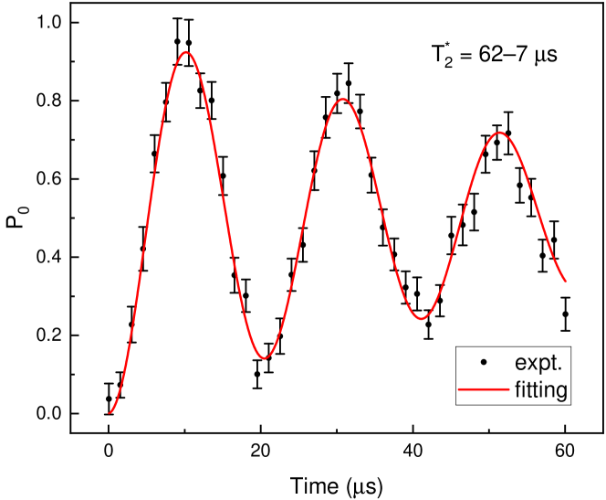
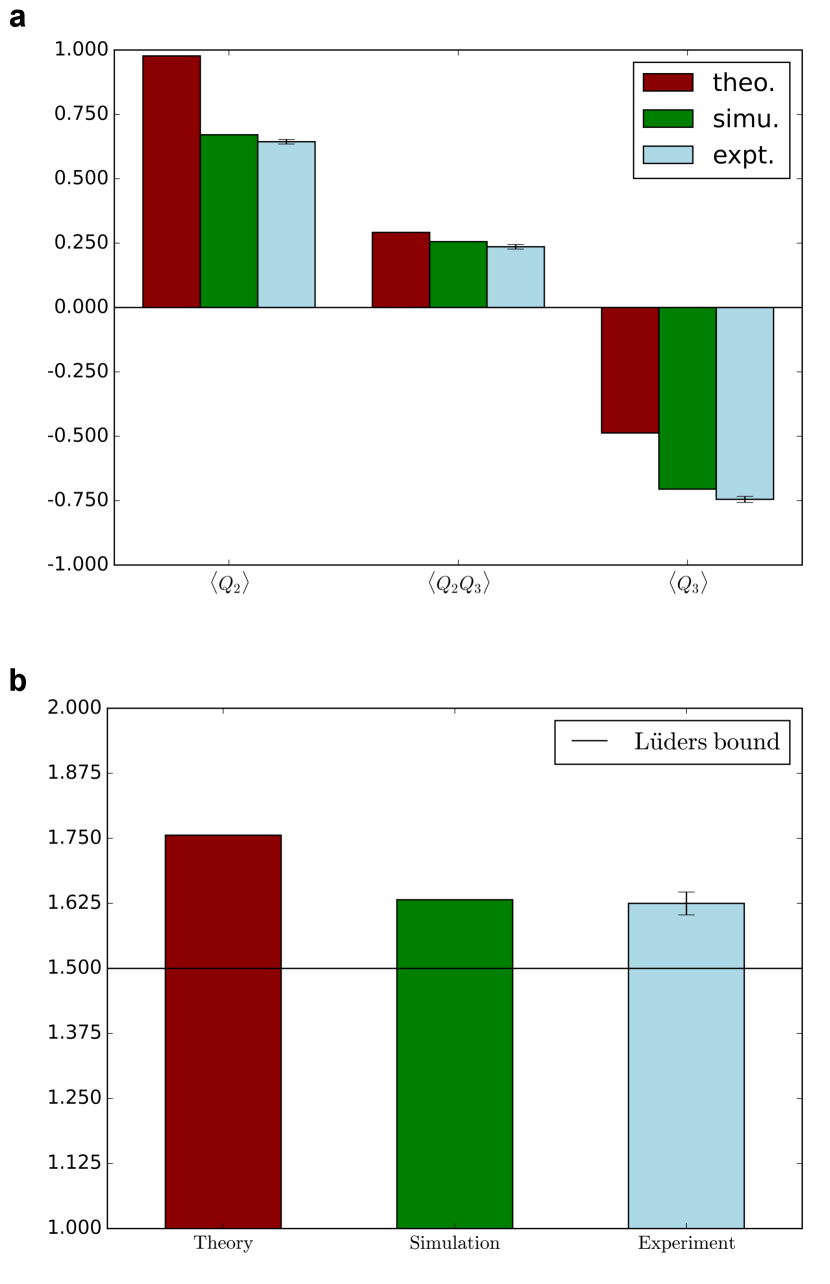
The maximal value of should be obtained when , corresponding evolution time under the Hamiltonian is . A major factor affecting the experimental results is the dephasing noise of the electron spin. Therefore, we utilized an isotopically purified ([12C]=99.999%) sample to implement our experiments. The dephasing time of the electron spin is measured to be 62(7) as shown in Fig. 3. Under this condition, the experimentally obtained values of , and for are shown in Fig. 4(a). The corresponding values of are shown in Fig. 4(b), where the red (left) bar is the ideal prediction according to Eq. (12), the green (middle) bar is the simulation result with dephasing noise and initialization imperfection, and the light blue (right) bar is the experimental result. At the point of the maximum violation, the experimental result is . The error, , is the standard deviation from the mean. This result exceeds the Lders bound of 1.5 with a level of confidence. Considering dephasing noise and imperfect initialization of ancilla qubit, the corresponding simulation result is and it is agrees with the experimental result (see Appendix C for detailed calculations).
In summary, we have experimentally demonstrated violation of LGI in a single spin three-level system beyond the Lders bound using the INRM scheme. The difference in experimental result from theoretical value is due to dephasing noise and imperfection of initialization of ancilla qubit. To improve the experimental result, the effect of dephasing noise can be suppressed by using the sample with long coherence time and the quantum control which can resist noise. Some other quantities such as the quantum witness can be measured for the further investigation of macrorealist theoriesSchild_2015 . We hope that our results in three-level system can extend to large scale system, paving the way to looking for macroscopic superposition state in high-dimensional system.
This work was supported by the National Key RD Program of China (Grants No. 2018YFA0306600 and No. 2016YFB0501603), the NNSFC (No. 81788101), the Chinese Academy of Sciences (Grants No. QYZDY-SSW-SLH004 and No. QYZDB-SSW-SLH005), and Anhui Initiative in Quantum Information Technologies (Grant No. AHY050000). X. R. thanks the Youth Innovation Promotion Association of Chinese Academy of Sciences for the support. Ya Wang thanks the Fundamental Research Funds for the Central Universities for the support.
I Appendix A: Characterizing the flip probability of the electron spin when nuclear spin is in a flip state
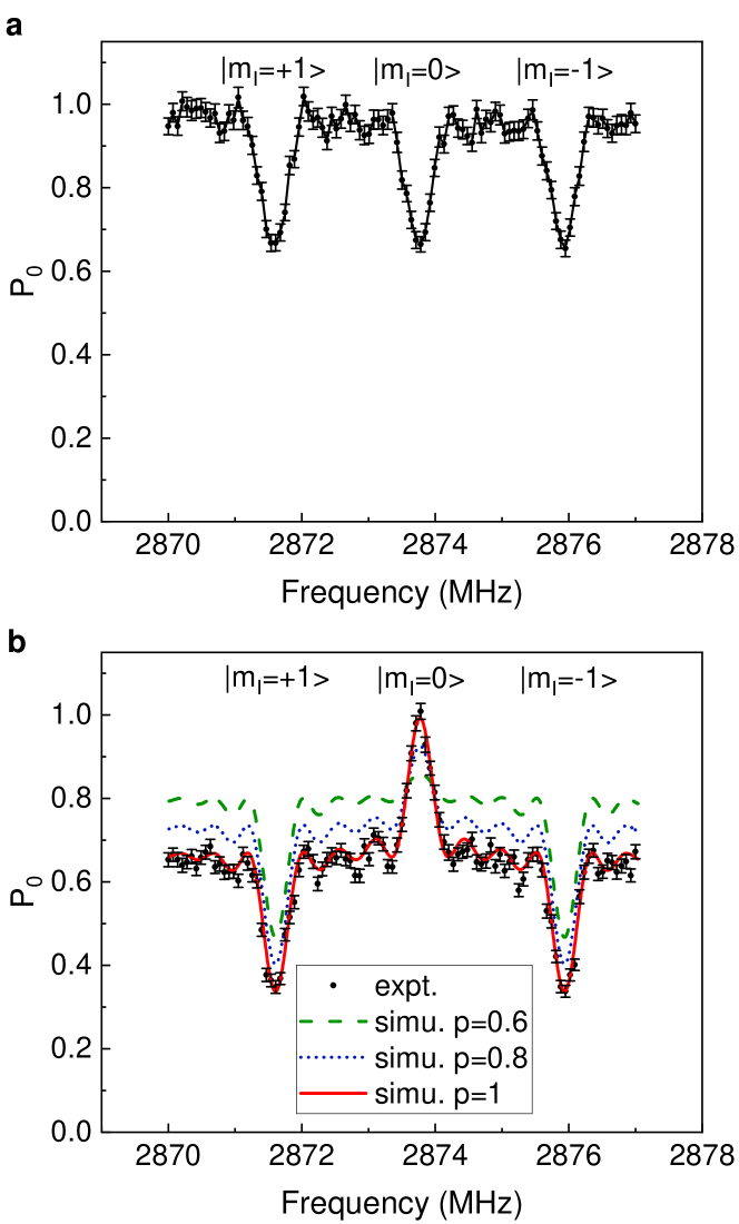
We implemented experiments to show the probability of the ancilla qubit flipped when nuclear spin is in a flip state. Before applying the controlled gate, the electron spin is initialized to the state. Thus the corresponding state population is 1. When sweeping the frequency of the microwave pulse, we observed three peaks as shown in Fig. 5a corresponding to three different states of the nuclear spin. Fig. 5b shows the results after implementing the controlled gate.
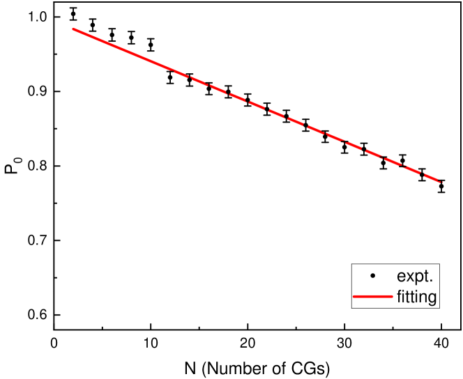
Compared to the simulation results, our results are quite different from the cases with probability 0.6 and 0.8, and agree well with the case of probability 1. In order to obtain a more precise probability , we performed an additional experiment which applied the controlled gates repeatedly. The dynamics of the quantum state was recorded. The population of state after repeated applications of controlled gates is shown in Fig. 6. The probability p of can be obtained by linear fitting.
II Appendix B: LG function obtained from the populations of the final states
At , three controlled gates are applied corresponding to three nuclear spin states. We postselect the ancilla qubit to remain in the state, which is not flipped. Therefore, the expectation value at is
| (B1) | ||||
The correlated expectation value is
| (B2) | ||||
In order to obtain , there is no need to apply the controlled gates at . We still postselect the state where the ancilla qubit does not flip. Therefore, the expectation value at is
| (B3) |
III Appendix C: Imperfections Considered in the Simulation Results
The imperfect polarization and the decoherence of the electron spin contribute to the difference between ideal and simulation results. At the magnetic field strength of 512 G, the spin state of the NV center is effectively polarized to . The polarization of electron spin and nuclear spin are 95% and 98%. Our experiment was implemented on a NV center in diamond which was isotopically purified ([12C]=99.999%). The dephasing time of the electron spin, is measured to be 62(7) . The experiments suffered from the dephasing noise during pulse sequences. There will be one more dephasing noise term, , in the practice Hamiltonian. The dephasing noise, , mainly comes from the Overhauser field (due to the interaction with the nuclear spin bath), the magnetic field fluctuation and the instability of the microwave frequency. The satisfies a Gaussian distribution with Rong_2015 . The simulation results are obtained with the consideration of initial polarization and the dephasing noise distribution .
References
- (1) A. J. Leggett and A. Garg, Phys. Rev. Lett. 54, 857 (1985).
- (2) A. J. Leggett, J. Phys. Condens. Matter. 14, R415 (2002).
- (3) A. J. Leggett, Rep. Prog. Phys. 71, 022001 (2008).
- (4) O. J. Maroney and C. G. Timpson, arXiv:1412.6139 (2014).
- (5) H. Katiyar, A. Brodutch, D. Lu, and R. Laflamme, New J. Phys. 19, 023033 (2017).
- (6) C. Budroni and C. Emary, Phys. Rev. Lett. 113, 050401 (2014).
- (7) G. Lders , Ann. Phys. (Amsterdam) 15, 663-670 (2006).
- (8) J. Dressel, C. J. Broadbent, J. C. Howell, and A. N. Jordan, Phys. Rev. Lett. 106, 040402 (2011).
- (9) A. Palacios-Laloy, F. Mallet, F. Nguyen, P. Bertet, D. Vion, D. Esteve, and A. N. Korotkov, Nat. Phys. 6, 442–447 (2010).
- (10) H. Katiyar, A. Shukla, K. R. K. Rao, and T. S. Mahesh, Phys. Rev. A 87, 052102 (2013).
- (11) K. K. Wang, C. Emary, X. Zhan, Z. H. Bian, J. Li, and P. Xue, Opt. Express 25, 31462 (2017).
- (12) R. E. George, L. M. Robledo, O. J. E. Maroney, M. S. Blok, H. Bernien, M. L. Markham, D. J. Twitchen, J. J. L. Morton, G. A. D. Briggs, and R. Hanson, Proc. Natl. Acad. Sci. 110, 3777 (2013).
- (13) G. C. Knee, S. Simmons, E. M. Gauger, J. J. L. Morton, H. Riemann, N. V. Abrosimov, P. Becker, H.-J. Pohl, K. M. Itoh, M. L. W. Thewalt, G. A. D. Briggs, and S. C. Benjamin, Nat. Commun. 3, 606 (2012).
- (14) C. Emary, N. Lambert, and F. Nori, Rep. Prog. Phys. 77, 016001 (2014).
- (15) Y. Wu, W. Liu, J. Geng, X. Song, X. Ye, C.-K. Duan, X. Rong, and J. Du, Science 364, 878-880 (2018).
- (16) V. Jacques, P. Neumann, J. Beck, M. Markham, D. Twitchen, J. Meijer, F. Kaiser, G. Balasubramanian, F. Jelezko, and J. Wrachtrup, Phys. Rev. Lett. 102, 057403 (2009).
- (17) G. Schild and C. Emary, Phys. Rev. A 92, 032101 (2015).
- (18) X. Rong, J. Geng, F. Shi, Y. Liu, K. Xu, W. Ma, F. Kong, Z. Jiang, Y. Wu and J. Du, Nat. Commun. 6, 8748 (2015).