Experimental Study on The Effect of Multi-step Deep Reinforcement Learning in POMDPs
Abstract
Deep Reinforcement Learning (DRL) has made tremendous advances in both simulated and real-world robot control tasks in recent years. This is particularly the case for tasks that can be carefully engineered with a full state representation, and which can then be formulated as a Markov Decision Process (MDP). However, applying DRL strategies designed for MDPs to novel robot control tasks can be challenging, because the available observations may be a partial representation of the state, resulting in a Partially Observable Markov Decision Process (POMDP). This paper considers three popular DRL algorithms, namely Proximal Policy Optimization (PPO), Twin Delayed Deep Deterministic Policy Gradient (TD3), and Soft Actor-Critic (SAC), invented for MDPs, and studies their performance in POMDP scenarios. While prior work has found that SAC and TD3 typically outperform PPO across a broad range of tasks that can be represented as MDPs, we show that this is not always the case, using three representative POMDP environments. Empirical studies show that this is related to multi-step bootstrapping, where multi-step immediate rewards, instead of one-step immediate reward, are used to calculate the target value estimation of an observation and action pair. We identify this by observing that the inclusion of multi-step bootstrapping in TD3 (MTD3) and SAC (MSAC) results in improved robustness in POMDP settings.
Keywords: Deep Reinforcement Learning, Partially Observable Markov Decision Processes, Multi-step Methods, Robot Learning, Robotics
1 Introduction
Deep Reinforcement Learning (DRL) has been applied to both discrete and continuous control tasks, such as game playing (Mnih et al., 2013, 2015, 2016), simulated robots (Lillicrap et al., 2015; Duan et al., 2016), and real world robots (Mahmood et al., 2018; Satheeshbabu et al., 2020). Although there have been tremendous advances in DRL, there are many challenges in applying DRL to real world robots (Henderson et al., 2018; Dulac-Arnold et al., 2021). In this paper, we focus on the challenge of partial observability of the observation space, which changes a given task from a Markov Decision Process (MDP) to a Partially Observable MDP (POMDP).
Many popular DRL algorithms are formulated for and only tested in MDP problems with well-engineered action and observation spaces, and reward functions. This results in a tendency (Zhang et al., 2019; Lopez-Martin et al., 2020; Gregurić et al., 2020) in practise to assume a task is an MDP and directly apply off-the-shelf DRL algorithms designed for MDPs. However, POMDPs are very common in novel and complex control tasks (Cassandra, 1998; Foka and Trahanias, 2007; Ong et al., 2009; Pajarinen et al., 2022) where a lack of knowledge of the structure of the dynamics, sensor limitations, missing data, etc. is typical. In practise, the design of a novel simulation environment to train policies in also requires engineers to make judgements in places where they may lack the confidence to identify if a given environment and observation/action space results in an MDP or POMDP, particularly when faced with a novel application, e.g., Living Architecture Systems (Meng, 2023). This uncertainty can result in the selection of sub-optimal policy training method (eg. DRL algorithms designed for MDPs applied to POMDPs and vice versa). This is particularly concerning, as DRL algorithms developed to handle POMDPs (Hausknecht and Stone, 2015; Lample and Chaplot, 2017; Igl et al., 2018), offer no guarantees or evidence to support that these algorithms also work well in MDPs.
This in turn results in two key challenges for practitioners. The first is that there is no handy tool to detect if a given task is an MDP or POMDP. Such a tool, would allow practitioners to select appropriate DRL algorithms for the detected task, or make adjustments to the task design, e.g., turning a POMDP into a MDP, to make it easier to be tackled by the state-of-the-art algorithms. The second challenge is the absence of DRL algorithms that work well in both MDPs and POMDPs.
This paper identifies an unexpected result when applying DRL algorithms developed for MDPs to POMDPs and exploits this to address the two aforementioned problems. Specifically, this paper shows that the unexpected result, that TD3 and SAC underperform PPO on MDP tasks modified to be POMDP, can be potentially used to detect if a given task is a MDP or POMDP.
Our findings also shed light on the effect of multi-step DRL in POMDPs and suggest that by using multi-step bootstrapping DRL algorithms designed for MDPs we can achieve better performance in POMDPs. We first present a motivating example in Section 4, where it is not known if a task is a MDP or POMDP. In Section 5 we hypothesize that TD3 and SAC are expected to outperform PPO on MDPs, but underperform PPO on POMDPs and design experiment to validate the the generalization of the finding in the previous section. In addition, in Section 6, we further formulate hypotheses on why PPOs outperforms TD3 and SAC on POMDPs and how to make TD3 and SAC perform better on POMDPs based on our analysis. Experiments are also designed accordingly to validate these hypotheses. The experimental results are presented in Section 7. Particularly, our experiments confirm the generalization of the finding on different tasks with various types of partial observability. Moreover, it is experimentally proven that by employing multi-step bootstrapping both TD3 and SAC demonstrate better performance on POMDPs. Following that, 8 further discusses the meaning of these findings and highlights the limitations of this work. At the end, Section 9 summarize the paper and points out some interesting future directions.
2 Related Work
MDP solutions obtained using DRL have enabled tremendous advancements. For MDPs with discrete action spaces, Deep Q-Network (DQN) (Mnih et al., 2013), Double DQN (Van Hasselt et al., 2016), Dueling DQN(Wang et al., 2016b), Actor Critic with Experience Replay (ACER)(Wang et al., 2016a) have been proposed and shown to achieve or exceed human performance. For continuous action spaces, Trust Region Policy Optimization (TRPO)(Schulman et al., 2015a), PPO (Schulman et al., 2017), Deep Deterministic Policy Gradient (DDPG)(Lillicrap et al., 2015), TD3 (Fujimoto et al., 2018), and SAC (Haarnoja et al., 2018) have been proposed. In addition, there are also DRL algorithms designed to work for both discrete and continuous action spaces, e.g., Advantage Actor Critic (A2C)(Mnih et al., 2016). There are also works applying DRL to a multi-agent system by modeling the system as a Decentralized MDP (Dec-MDP) (Beynier et al., 2013). However, all these algorithms are designed for and tested with MDPs that are well engineered with fully-observable states for most cases, and it is unclear whether these algorithms will work well or to what extent they can maintain their relative performance in POMDPs. In this paper, we focus on continuous control tasks and show that PPO, SAC, TD3 do not maintain their relative performance in POMDPs, with PPO underperforming SAC and TD3 in MDPs but outperforming SAC and TD3 in POMDPs.
POMDPs have gained extensive attentions in the community and been investigated within both model-free (Hausknecht and Stone, 2015; Lample and Chaplot, 2017; Meng et al., 2021b) and model-based (Igl et al., 2018; Singh et al., 2021; Shani et al., 2013) DRL, including POMDPs with discrete(Baisero and Amato, 2021) or continuous(Ni et al., 2021) action spaces. Ni et al. (2021) empirically shows that recurrent model-free RL can be a strong baseline for many POMDPs. Subramanian et al. (2022) proposes a theoretical framework for approximate planning and learning in POMDPs, where an approximate information state can be used to learn an approximately optimal policy. In addition, multi-agent system can also be modeled as a Decentralized POMDP (Dec-POMDP) and approached by DRL algorithms (Beynier et al., 2013; Oliehoek et al., 2016), which demonstrates the broad application of DRL in POMDPs.
Multi-step methods (also called n-step methods/bootstrapping) refer to RL algorithms that utilize multi-step immediate rewards to estimate the bootstrapped value of taking an action in a state. These have been investigated in the literature for improving reward signal propagation (van Seijen, 2016; Mnih et al., 2016; De Asis et al., 2018; Hessel et al., 2018) leading to faster learning speed. Multi-step bootstrapping has also been shown to help to alleviate the over-estimation problem in Meng et al. (2021a). However, to the best of our knowledge, there is no work connecting multi-step methods to their potential ability to capture temporal information when solving POMDPs. In this work, we show that PPO with multi-step bootstrapping outperforms TD3 and SAC that only using 1-step bootstrapping in POMDPs. We also empirically show that multi-step bootstrapping helps TD3 and SAC to perform better in POMDPs.
From the related work on DRL for MDPs and POMDPs, we can see that MDPs and POMDPs are normally tackled separately in DRL and little work is done on bridging MDPs and POMDPs and their solvers. Even though there are some efforts on solving POMDPs by using MDP solvers in conjunction with imitation learning (Yoon et al., 2008; Littman et al., 1995), (Arora et al., 2018) shows that multi-resolution information gathering cannot be addressed using MDP based POMDP solvers by only focusing on one specific task. In addition to inventing algorithms that work for both MDPs and POMDPs, there is also effort studying how to reducing PODMPs to MDPs. For example, Sandikci (2010) studies the reduction of a POMDP to a MDP by exploiting grid approximation, but this assumption on a finite discrete belief state space limits applications to continuous state spaces.
Successfully applying DRL to real applications involves many design choices, with state representation particularly important. For example, (Reda et al., 2020) studies the environment design, including the state representations, initial state distributions, reward structure, control frequency, episode termination procedures, curriculum usage, the action space, and the torque limits, that matter when applying DRL. They empirically show these design choices can affect the final performance significantly. In addition, Ibarz et al. (2021) focuses on investigating the challenges of training real robots with DRL, compared to simulation. As another work related to state representation, Mandlekar et al. (2021) studies the factors that matter in learning from offline human demonstrations, where observation space design is highlighted as a particularly prominent aspect. These works aim to comprehensively cover broader topics in applying DRL, but in this work we mainly focus on the partial observability problem during DRL for robot control. Moreover, we try to reproduce the problem encountered when applying DRL to novel robots using benchmark tasks where the problem can be more easily reproduced and studied.
As this paper conducts experimental study across both MDPs and POMDPs, it is worth noting bench-marking efforts for DRL algorithms. Particularly, we note that DRL algorithms are often separately bench-marked for MDPs and POMDPs (Duan et al., 2016; Ni et al., 2021). This introduces uncertainty around the performance of DRL algorithms benchmarked on MDPs in POMDPs and vice versa. We speculate that this phenomena is partly due to the unbalanced availablity of testbeds for MDPs and POMDPs. There are many MDP testbeds, e.g., Gymnasium (Towers et al., 2023), DeepMind Control Suite (Tunyasuvunakool et al., 2020), and many more https://github.com/clvrai/awesome-rl-envs than POMDP testbeds. As an example testbed for discrete action spaces, Shao et al. (2022) proposes Mask Atari for deep reinforcement learning as a POMDP benchmark, where the observation of Atari 2600 games are manipulated by masks in order to create POMDPs. For continuous action spaces, Morad et al. (2023) provides Popgym to benchmark partially observable reinforcement learning. In additional to the availability of MDP and POMDP testbeds, MDP testbeds are commonly benchmarked in Duan et al. (2016); Weng et al. (2022); Hill et al. (2018), but because the POMDP bestbeds are not so popular, there is not much popular benchmarks for them neither. This paper uses POMDP testbeds modified from MDP testbeds in Gymnasium, exploiting similar techniques to those proposed by Meng et al. (2021b).
3 Background
A Markov Decision Process (MDP): is a sequential decision process defined as a 4-tuple , where is the state space, is the action space, is the transition probability that action in state at time will lead to a new state at time , and provides the immediate reward indicating how good taking action is in state after transitioning to a new state . In a MDP, it is assumed that the state transitions defined in satisfy the Markov property, i.e. the next state only depends on the current state and the action . Normally, the state is not accessible to an agent, but its representation is given. When the observation fully captures the current state , we call this a fully observable MDP. However, when the observation cannot fully represent the current state , we call the decision process a Partially Observable Markov Decision Process (POMDP). In some cases, using a history of past observations and/or actions and/or rewards up to time as a new observation can reduce a POMDP to MDP. For example, for tasks where the velocity is part of the system state, using a history of past positions of a robot as the observation can make the POMDP, where only position is included in its observation, a MDP. For these cases, history aids with dealing with partial observability.
Reinforcement Learning (RL): Sutton and Barto (2018) studies how to solve MDPs or POMDPs, without requiring the transition dynamics to be known. Specifically, an agent observes at time , then decides to take action according to its current policy . Once the action is taken, the agent observes a new observation and receives a reward signal from the environment. By continuously interacting with the environment, the agent learns an optimal policy to maximize the expectation of the discounted return starting from initial observation , where the discount factor is used to balance the short-term vs. long-term return.
There are three functions that are commonly used in RL algorithms. A state-value function of a state under a policy is the expected return when starting in and following thereafter, which can be formally defined by . An action-value function of taking action in state and following afterwards can be defined as . The advantage of taking action in state is defined as when following a policy . For these functions, if the state is not directly observable, its representation will be used. To simplify the notation, for the rest of this paper, we will use to represent .
3.1 Deep Reinforcement Learning
Deep Reinforcement Learning (DRL) employs Deep Neural Networks to represent these value functions and/or policy. In this paper, we will use three of the most popular DRL algorithms which will be briefly introduced in the following.
Both Soft Actor-Critic (SAC) (Haarnoja et al., 2018) and Twin Delayed Deep Deterministic Policy Gradient (TD3) (Fujimoto et al., 2018) are off-policy actor-critic DRL approaches. Both employ two neural networks to approximate two versions of the state-action value function (named critics) parameterized by . Learning two versions of the critic is used to address the function approximation error by taking the minimum over the bootstrapped Q-values in the next observation . Unlike TD3, SAC gives a bonus reward to an agent at each time step, proportional to the entropy of the policy at that timestep. In addition, TD3 learns a deterministic policy parameterized by , whereas SAC learns a stochastic policy parameterized by . Given a mini-batch of experiences uniformly sampled from the replay buffer , the target bootstrapped Q-value of taking action in observation can be defined as follows:
| (1) |
where the target Q-value functions are parameterized by , for TD3 with target policy and for SAC with target policy , and balances the maximization of the accumulated reward and entropy. For TD3 . Then, can be optimized by minimizing the expected difference between the prediction and the bootstrapped value with respect to parameters , following . For TD3, the policy is optimized by maximizing the expected Q-value over the mini-batch of with respect to the policy parameter , following
| (2) |
and for SAC the policy is updated to maximize the expected Q-value on where is sampled from policy and the expected entropy of in observation as
| (3) |
Proximal Policy Optimization (PPO) (Schulman et al., 2017) optimizes a policy by taking the biggest possible improvement step using the data collected by the current policy, but at the same time limiting the step size to avoid performance collapse. A common way to achieve this is to attenuate policy adaptation. Formally, for a set of observation and action pairs collected from the environment based on the current policy , the new policy is obtained by maximizing the expectation over the loss function with respect to the policy parameter as . The loss function is defined as
| (4) | ||||
where , is a small hyperparameter that roughly says how far away the new policy is allowed to go from the current one, and is the advantage value. A common way to estimate the advantage is called generalized advantage estimator GAE() (Schulman et al., 2015b), based on the -return and the estimated state-value in observation as . The is defined by
| (5) |
where balances the weights of different multi-step returns and the summation of the coefficients satisfies . Particularly, is defined as that is bootstrapped by state-value in observation . The state-value function is optimized to minimize the mean-square-error between the predicted state value and the Monte-Carlo return as , where the Monte-Carlo return is defined as
| (6) |
which is calculated based on the experiences collected by the current policy. In Eq. 6, indicates after steps if the agent reached the terminal state or not, and is the next observation after steps.
Multi-step Methods (also called -step methods) (Sutton and Barto, 2018) refer to RL algorithms utilizing multi-step bootstrapping. Formally, for a multi-step bootstrapping where is the step size after which a bootstrapped value will be used, the -step bootstrapping of observation and action pair can be defined as where . Note that when , it reduces to 1-step bootstrapping, which is commonly used in Temporal Difference (TD) based RL.
4 Exemplar Robot Control Problem
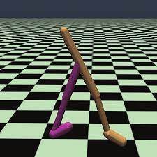
In this section, we will provide a motivating example highlighting the challenge of applying DRL to tasks with sensor noise which leads to POMDP. The Walker2D (as shown in Fig. 1(a)) Mujoco environment in Gymnasium (https://gymnasium.farama.org) is a two-legged walking robot in 2D, where the objective is to walk forward as fast as possible by applying torques on the six hinges connecting the seven body parts. The observation of the original task consists of the positions and velocities of different body parts of the robot, which fully represents the state of the robot and makes the task a MDP. The original task is good for validating the DRL algorithms, but it is unrealistic in reality because there is always sensory noise in the observation for a real robot. Therefore, to make it closer to the real world a modified task is created, whose observation is formed by adding random Gaussian noise with zero mean and standard deviation to the original observation as , a setting of more practical relevance. The inclusion of random observation noise means the new observation of the modified task is a noisy representation of the state, and hence the task is a POMDP.
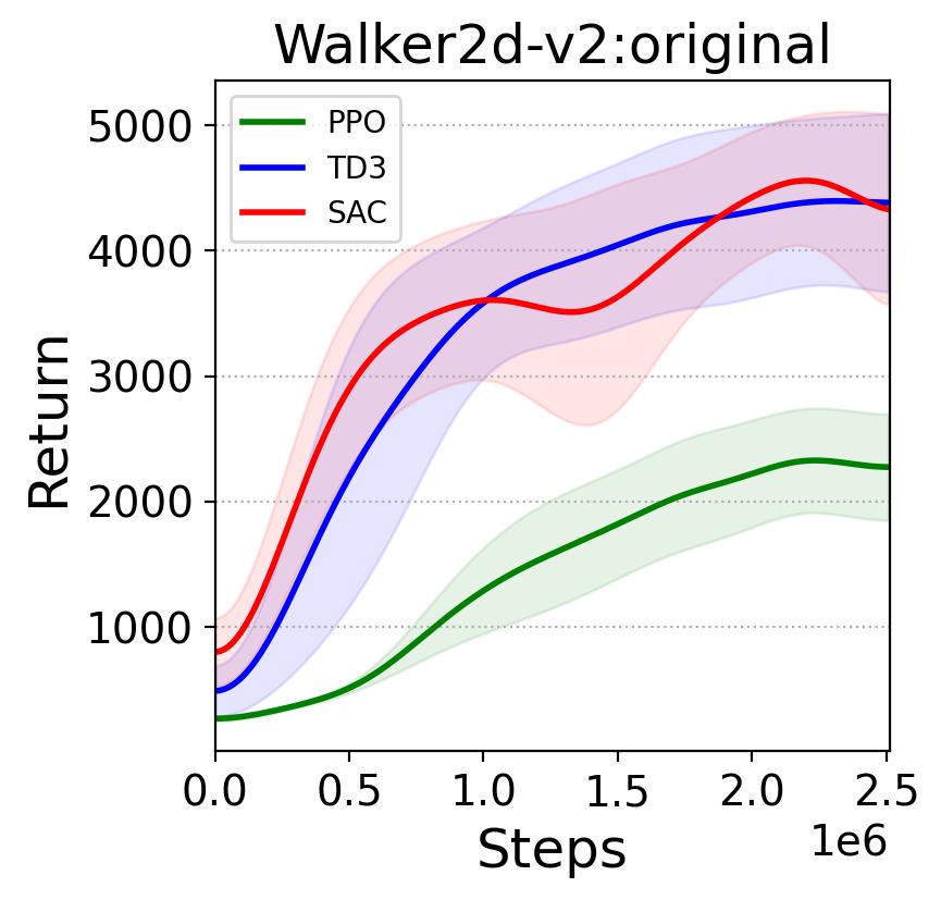
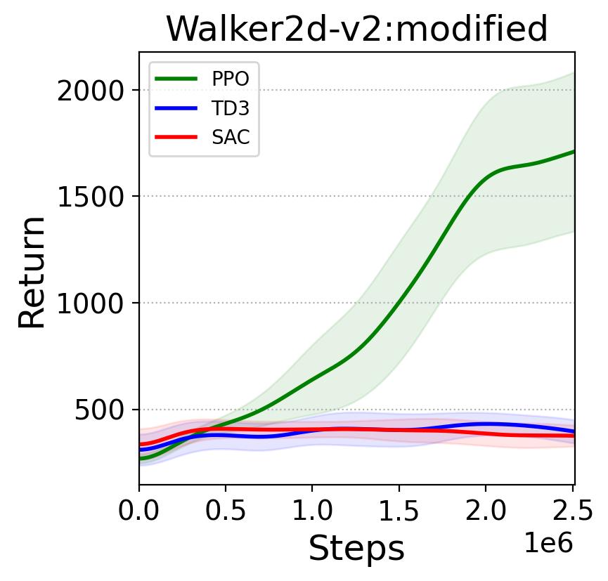
Given a control task, when applying DRL algorithms to it, it is common to start with state-of-the-art DRL algorithms, e.g., the TD3, SAC, and PPO approaches introduced in Section 3. Based on the results reported by Fujimoto et al. (2018); Haarnoja et al. (2018), one may expect that both TD3 and SAC would outperform PPO on the modified task, given relative performance on the original MDP task illustrated in Fig. 1(b). However, surprisingly, TD3 and SAC perform much worse than PPO on the POMDP version of Walker2D, as shown in Fig. 1(c). A similarly counter-intuitive result is also encountered by Meng (2023), when applying these algorithms to Living Architecture Systems. TD3, SAC and PPO are all general DRL algorithms with no special consideration for handling a POMDP, but the results shown in 1 indicate that PPO is less sensitive to the partial observation setting than TD3 and SAC. To further investigate whether the observation in the exemplar task generalizes to other tasks and to interpret these results, we will reproduce the exemplar test with POMDP variations of other benchmark tasks from Gymnasium, in Section 7. To ease the reference in the rest of this work, we summarize the Expected Result and the Unexpected Result in Table 1.
| Expected Result | TD3 and SAC outperform PPO on MDP tasks modified to be POMDP. |
| Unexpected Result | TD3 and SAC underperform PPO on MDP tasks modified to be POMDP. |
Because the noisy sensor setting in the exemplar control task introduced in Section 4 is common in practise, it is worth investigating to what extent the Unexpected Result will generalize to other benchmark tasks and other types of POMDPs studied in RL literature and understand its underlying causes.
5 Generalization of the Unexpected Result on Other Tasks
To examine the generalization of the result shown in the previous section, especially the Unexpected Result , we reproduce these findings in three additional benchmark control tasks detailed in Section 7. To experimentally validate the generalization, we formally make the Hypothesis 1 as:
Hypothesis 1
If the partial observability introduced by adding random noise caused the unexpected results relative to the expection on MDP, then similar results should be reproducible on MDP vs. POMDP versions of other benchmark tasks. Concretely, TD3 and SAC are expected to outperform PPO on MDPs, but underperform PPO on POMDPs.
If Hypothesis 1 is supported by the experiment, it means that applying DRL algorithms in real-world robot control cannot directly exploit the evidence obtained by the RL community that TD3 and SAC are better than PPO. What’s more, when it is observed that PPO outperforms TD3 and SAC on a given task, this should be taken as evidence that the task at hand might be a POMDP rather than a MDP. Therefore, either the design of the task observation space should be amended to turn the POMDP into an MDP, or DRL algorithms for specifically for POMDPs should be employed.
6 Analysing and Improving Robustness to Partial Observability
To understand the cause of the Unexpected Result , we analyze the key differences between PPO and TD3 or SAC. Then, we propose hypotheses based on the analysis and experimentally validate these. The two key differences between PPO and TD3 or SAC are as follows:
Diff 1
PPO exploits multi-step bootstrapping for both advantage and state-value function estimation, while TD3 and SAC only use one-step bootstrapping for action-value function estimation.
Diff 2
PPO updates its policy conservatively leading to gentle exploration, TD3 explores by adding Gaussian action noise with fixed standard deviation to its deterministic policy, whereas SAC always encourages exploration.
In the rest of this section, we will make hypotheses based on our analysis on these features and propose methods to experimentally validate these hypotheses.
6.0.1 The Potential Effect of Multi-step Bootstrapping on Passing Temporal Information
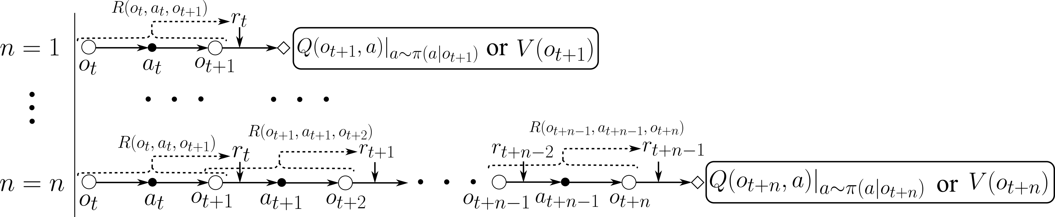
For Diff 1, PPO uses -return defined in Eq. 5, which is a weighed average of -step returns where , to calculate the advantage of taking action in observation , and then uses the Monte-Carlo return defined in Eq. 6 to update its state-value function. However, TD3 and SAC only use -step bootstrapping to calculate their target Q-value as defined in Eq. 1. Fig. 2 illustrates -step bootstrapping with different values, where the immediate rewards and the bootstrapped value are discounted 111For clarity, we did not draw discount factor in the figure. and added together.
On MDPs, it is known that multi-step bootstrapping can propagate the learning signal, i.e., reward, faster (Sutton and Barto, 2018) leading to faster learning speed, and in DRL multi-bootstrapping (Meng et al., 2021a) also has the effect of alleviating the overestimation problem. However, neither of these explain the Unexpected Result . Concretely, considering the dense reward signal used in the task, even without the faster learning signal propagation endowed by the multi-step bootstrapping, TD3 and SAC should also improve gradually, which is not observed in Fig. 1(c). In addition, both TD3 and SAC utilize the minimum of the two critics (Eq. 1) to calculate the bootstrapped Q-value so that they are less likely to be affected by the overestimation problem.
Based on this analysis, we postulate that multi-step bootstrapping can pass temporal/sequential information that cannot be captured by one-step bootstrapping, and that causes the RL algorithms utilizing multi-step bootstrapping to be less sensitive to partial observation of the underlying state and able to achieve better performance. This assumption is inspired by the two empirical facts that (1) when the observation is a partial representation of the underlying state, a sequence of observations may form a better representation of the state, e.g., in Meng et al. (2021b) using an observation of simply concatenated multi-step observations significantly outperforms one-step observation on POMDPs, and (2) the dense reward signal can be roughly viewed as a one-dimensional state-transition abstraction of . More detailed on the second point can be found in Appendix A.1.
Because multi-step bootstrapping makes use of multiple rewards to calculate the target Q-value, the reward can be seen as an approximation of the state-transition, and it is likely this will further help to capture some missed temporal information, making DRL algorithms employing multi-step bootstrapping, e.g., PPO, less sensitive than those using one-step bootstrapping, e.g., TD3 and SAC. We validate this assumption experimentally by testing the hypothesis proposed in this section.
Hypothesis 2
The -return (Eq. 5) and Monte-Carlo return (Eq. 6) based on multi-step bootstrapping222-return is a weighted mixture of various -step bootstrappings, and Monte-Carlo return is a T-step bootstrapping employed in PPO leads to robustness to POMDP settings, therefore (1) multi-step/-step versions of TD3 and SAC with should also improve robustness to POMDPs when compared to their vanilla versions, and (2) replacing the -return and Monte-Carlo return with 1-step bootstrapping should cause PPO’s performance to decrease when moving from a MDP to a POMDP.
To empirically verify (1) of the Hypothesis 2, we investigate the performance of the multi-step (also known as -step) variants of vanilla TD3 and SAC, namely Multi-step TD3 (MTD3) (Tang, 2020) and Multi-step SAC (MSAC) (Bai, 2021), on various tasks. Specifically, instead of sampling a mini-batch of 1-step experiences, we sample a mini-batch of -step experiences. Then, we replace the target Q-value calculation defined in Eq. 1 with the -step bootstrapping defined as
| (7) |
where and for MTD3 and MSAC, respectively, for MTD3, and the policy update is the same as that for TD3 and SAC. For (2) of the Hypothesis 2, we replace both -return and Monte-Carlo return with -step return , i.e., and where when only 1-step bootstrapping is used.
In Hypothesis 2, we assume multi-step bootstrapping can improve DRL algorithms’ robustness to POMDP, inspired by the observation that the concatenation of multi-step observations significantly improves DRL algorithms’ performance on POMDPs and the intuition that reward can be seen as an approximation to the state-transition. Given that, it is natural to analogously ask if replacing the original one-step reward with an accumulated reward or can achieve similar performance improvement, since this can also incorporate multi-step rewards that may possibly capture some temporal information. In other words, Hypothesis 2 expects performance improvement when replacing Eq. 8 with Eq. 9, and similarly we can expect performance improvement when replacing Eq. 8 with Eq. 10 and comparable performance between Eq. 9 and Eq. 10.
| (8) |
| (9) |
| (10) |
Following this idea, we make a hypothesis as follows:
Hypothesis 3
If multi-step rewards can capture temporal information, the performance on tasks with accumulated reward over a few steps should be better than that on environments with one-step reward, i.e., the original reward, and achieve comparable performance to algorithms using multi-step bootstrapping on environments with one-step reward.
To validate Hypothesis 3, in Eq. 10 we modified the original task reward in time step , where max_step indicates the maximum episode steps, as an accumulated reward or of -step () rewards as follows:
| (11) |
and
| (12) |
where Eq. 11 and Eq. 12 correspond to the average and summation of the rewards. The modified reward or will be used for policy learning, but for performance comparison the original reward will be used.
6.0.2 The Potential Effect of Exploration Strategies
In terms of Diff 2, PPO updates its policy conservatively controlled by hyper-parameter in Eq. 4, where the smaller the the more conservative the policy update. SAC optimizes its policy to encourage exploration by maximizing the policy entropy controlled by a hyper-parameter as shown in Eq. 3, where the higher the is the more exploratory the policy will be. As for TD3, it uses a deterministic policy and its policy is simply optimized to maximize the estimated Q-value as in Eq. 2. For the exploration, TD3 adds an action noise to its policy following where the exploratory action is clipped to its value range , and controls how exploratory the action will be.
Hypothesis 4
If the less exploratory policy of PPO leads to the robustness in POMDP settings, (1) reducing the exploration in TD3 and SAC should also make these robust to POMDP, while (2) increasing the exploration of PPO should make it less effective in POMDPs.
To validate Hypothesis 4, we can adjust the action noise hyper-parameter of TD3 and the entropy coefficient hyper-parameter of SAC and see how this will affect their performance when moving from MDP to POMDP. For PPO, we can increase the clip ratio in Eq. 4 to allow the policy to update further away from the current policy.
6.0.3 Compound Effect of Multi-step Bootstrapping, Exploration Strategy, and/or Others
7 Experiments


| Name | Description | Hyper-params |
| MDP | Original task | |
| POMDP-RV | Remove all velocity-related entries in the observation space. | |
| POMDP-FLK | Reset the whole observation to 0 with probability . | |
| POMDP-RN | Add random noise to each entry of the observation. | |
| POMDP-RSM | Reset an entry of the observation to 0 with probability . | |
| Note: the POMDP-version tasks only transform the observation space of the original task, but leave the reward signal unchanged, which means the reward signal is still based on the original observations. This enables fair comparison across the performances of an agent in both the MDP and POMDP settings. | ||
The tasks investigated in this paper are from Gymnasium MuJoCo Environment, including Ant, HalfCheetah and Hopper, in addition to the Walker2D, as shwon in Fig. 3. Moreover, in addition to the random noise version (called POMDP-RN) of the modified tasks, we also study other variations of the original tasks as shown in Table 7, as proposed in Meng et al. (2021b). Specifically, the POMDP-RemoveVelocity (POMDP-RV) is designed to simulate the scenario where the observation space is not well designed, which is applicable to a novel control task that is not well-understood by researchers and therefore the designed observation may not fully capture the underlying state of the robot. The POMDP-Flickering (POMDP-FLK) models the case where remote sensor data is lost during long-distance data transmission. The case when a subset of the sensors are lost is simulated in POMDP-RandomSensorMissing (POMDP-RSM). Sensor noise is simulated in POMDP-RandomNoise (POMDP-RN). With these setups, we obtain 4 MDPs and 16=44 POMDPs.
The neural network structures and hyper-parameters of PPO, TD3, and SAC are the same as the implementation in OpenAI Spinning Up (https://spinningup.openai.com) documentation, and the source code of this paper can be found at https://github.com/LinghengMeng/m_rl_pomdp. MTD3() and MSAC() follow the implementation of TD3 and SAC, but use multi-step (also called -step) bootstrapping to update their Q-value function. The in the bracket indicates the step size in multi-step bootstrapping. LSTM-TD3() (Meng et al., 2021b) is also compared to see how the MTD3() and MSAC() perform compared to an algorithm specifically designed for dealing with POMDPs, where indicates the memory length (default ). More details on the hyper-parameters of the algorithms can be found in Appendix A.2. The results shown in this section are based on three random seeds. For better visualization, learning curves are smoothed by a 1-D Gaussian filter with .
| Task | Algorithms | ||||||
| Name | Version | PPO | TD3 | SAC | MTD3(5) | MSAC(5) | LSTM- TD3(5) |
| Ant | MDP | 476.99 | ✓ 4773.70 | ✓ 5614.10 | ✓ 3236.93 | ✓ 5000.62 | ✓ 4070.03 |
| POM-FLK | 396.67 | ✓ 1087.10 | ✓ 936.85 | ✓ 1693.12 | ✓ 2922.37 | ✓ 2658.81 | |
| POM-RN | 331.50 | ✓ 1051.60 | ✓ 1150.13 | ✓ 1078.68 | ✓ 2679.30 | ✓ 1095.33 | |
| POM-RSM | 383.02 | ✓ 1045.62 | ✓ 885.80 | ✓ 2048.93 | ✓ 3450.29 | ✓ 1164.97 | |
| POM-RV | 1997.48 | ✗ 1321.32 | ✗ 949.46 | ✓ 2557.28 | ✓ 2949.87 | ✗ 1325.87 | |
| HalfCheetah | MDP | 2897.89 | ✓ 9587.33 | ✓ 10419.59 | ✓ 5442.85 | ✓ 7270.04 | ✓ 8494.11 |
| POM-FLK | 1045.15 | ✓ 1141.83 | ✗ 103.27 | ✓ 1118.23 | ✓ 3397.47 | ✓ 1515.97 | |
| POM-RN | 2876.18 | ✓ 4009.17 | ✓ 3950.56 | ✓ 4961.27 | ✓ 4931.28 | ✓ 3108.72 | |
| POM-RSM | 2162.40 | ✗ 1149.96 | ✗ 50.62 | ✗ 1892.19 | ✓ 4603.68 | ✗ 1331.18 | |
| POM-RV | 2659.48 | ✗ 1424.24 | ✗ 157.48 | ✓ 2839.08 | ✗ 2393.62 | ✓ 3432.32 | |
| Hopper | MDP | 2602.18 | ✓ 3674.87 | ✓ 3575.86 | ✓ 3474.84 | ✓ 3588.95 | ✗ 2353.90 |
| POM-FLK | 1204.44 | ✗ 519.98 | ✗ 530.76 | ✗ 759.73 | ✗ 804.94 | ✓ 3400.00 | |
| POM-RN | 2360.31 | ✗ 597.15 | ✗ 584.08 | ✗ 1579.21 | ✗ 1569.69 | ✓ 2912.29 | |
| POM-RSM | 2733.00 | ✗ 1057.91 | ✗ 648.71 | ✗ 2237.73 | ✗ 2018.09 | ✗ 585.72 | |
| POM-RV | 848.52 | ✗ 532.99 | ✓ 1029.32 | ✗ 392.43 | ✗ 741.32 | ✗ 223.49 | |
| Walker2d | MDP | 3067.91 | ✓ 4902.00 | ✓ 4988.70 | ✓ 4838.84 | ✓ 5270.83 | ✓ 4591.12 |
| POM-FLK | 1241.49 | ✗ 569.78 | ✗ 577.98 | ✗ 639.63 | ✗ 819.88 | ✓ 3829.75 | |
| POM-RN | 2290.53 | ✗ 673.22 | ✗ 643.80 | ✓ 3194.54 | ✓ 2476.99 | ✓ 2617.48 | |
| POM-RSM | 1559.80 | ✗ 669.06 | ✗ 915.44 | ✓ 3228.56 | ✓ 3420.19 | ✓ 3820.27 | |
| POM-RV | 1603.86 | ✗ 735.30 | ✗ 1151.56 | ✓ 1908.67 | ✓ 2109.97 | ✓ 3360.62 | |
| Note: POM stands for POMDP. | |||||||
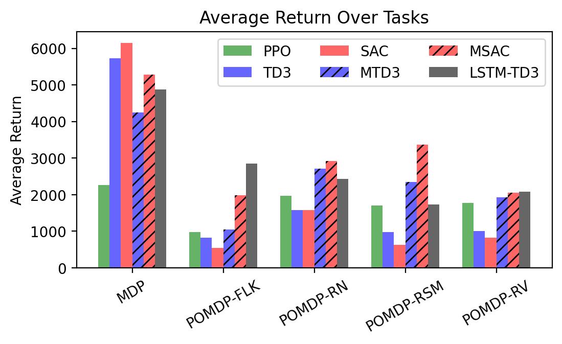
| Task | Algorithms | |||||
| PPO | TD3 | SAC | MTD3(5) | MSAC(5) | LSTM-TD3(5) | |
| MDP | 2261.24 | ✓ 5734.48 | ✓ 6149.56 | ✓ 4248.36 | ✓ 5282.61 | ✓ 4877.29 |
| POMDP-FLK | 971.49 | ✗ 829.67 | ✗ 537.22 | ✓ 1052.68 | ✓ 1986.16 | ✓ 2851.13 |
| POMDP-RN | 1964.63 | ✗ 1582.78 | ✗ 1582.14 | ✓ 2703.43 | ✓ 2914.32 | ✓ 2433.46 |
| POMDP-RSM | 1709.55 | ✗ 980.64 | ✗ 625.14 | ✓ 2351.85 | ✓ 3373.06 | ✓ 1725.54 |
| POMDP-RV | 1777.33 | ✗ 1003.46 | ✗ 821.95 | ✓ 1924.37 | ✓ 2048.70 | ✓ 2085.57 |
7.1 Results on the Generalization of the Unexpected Result on Other Tasks
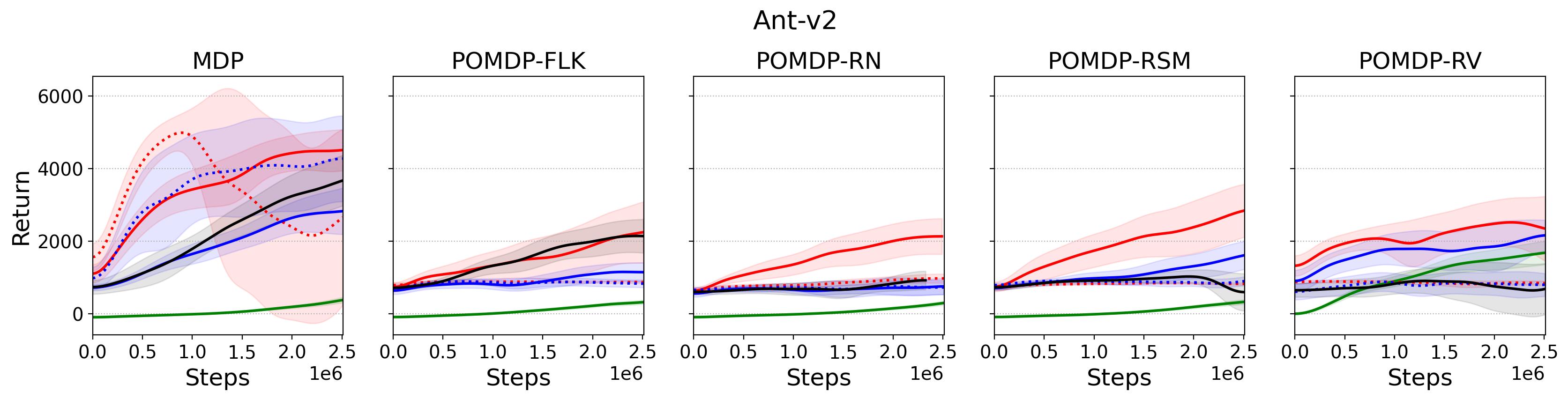
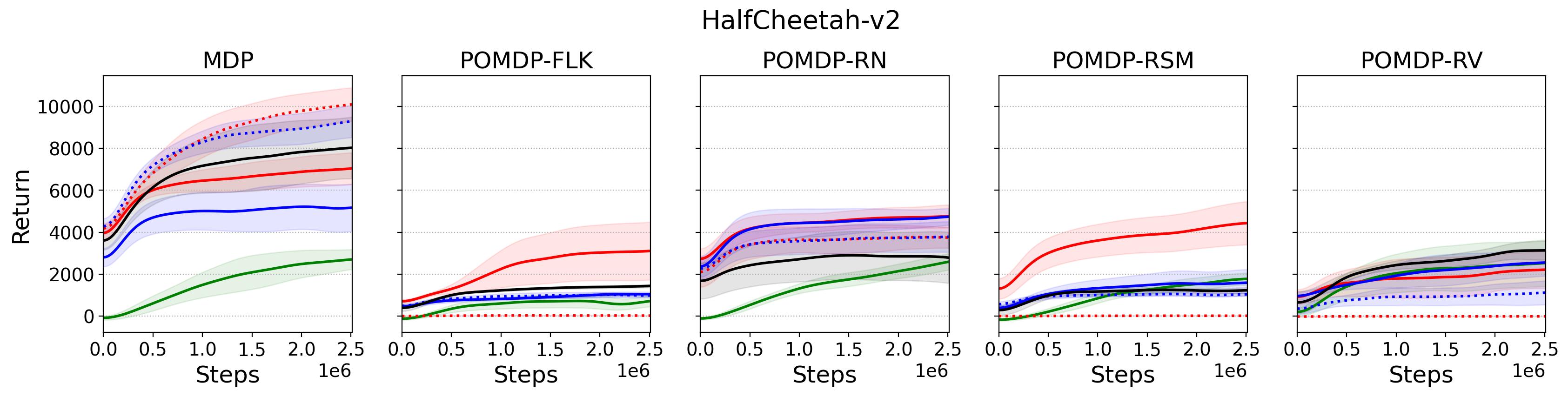
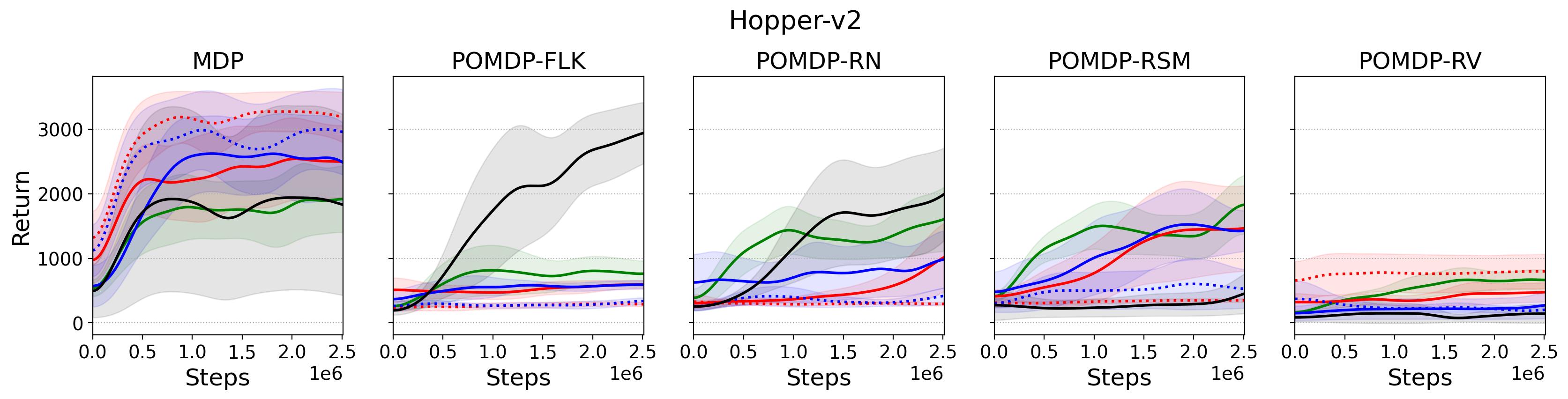
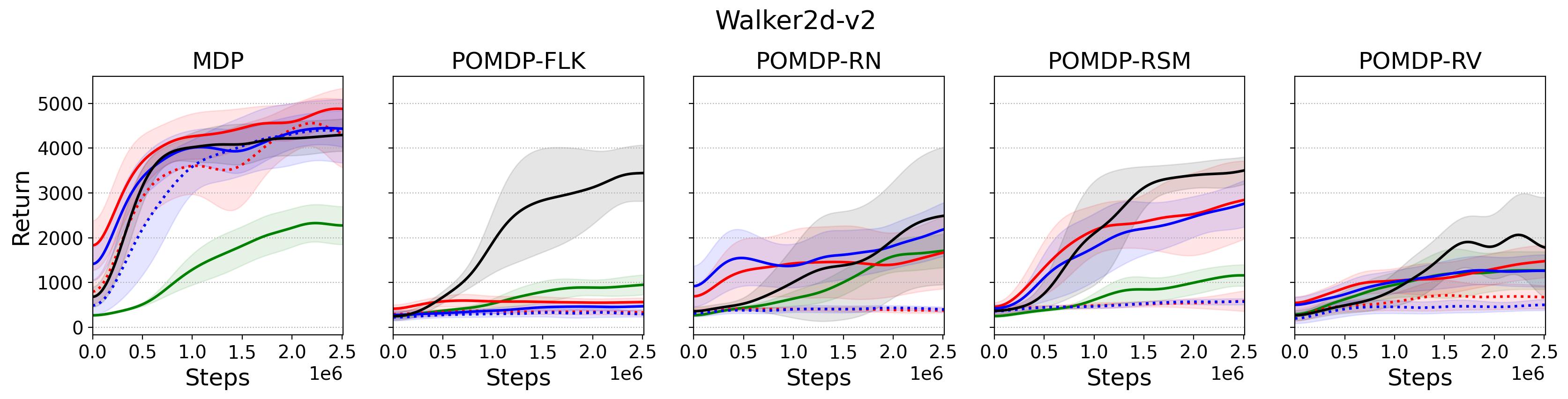
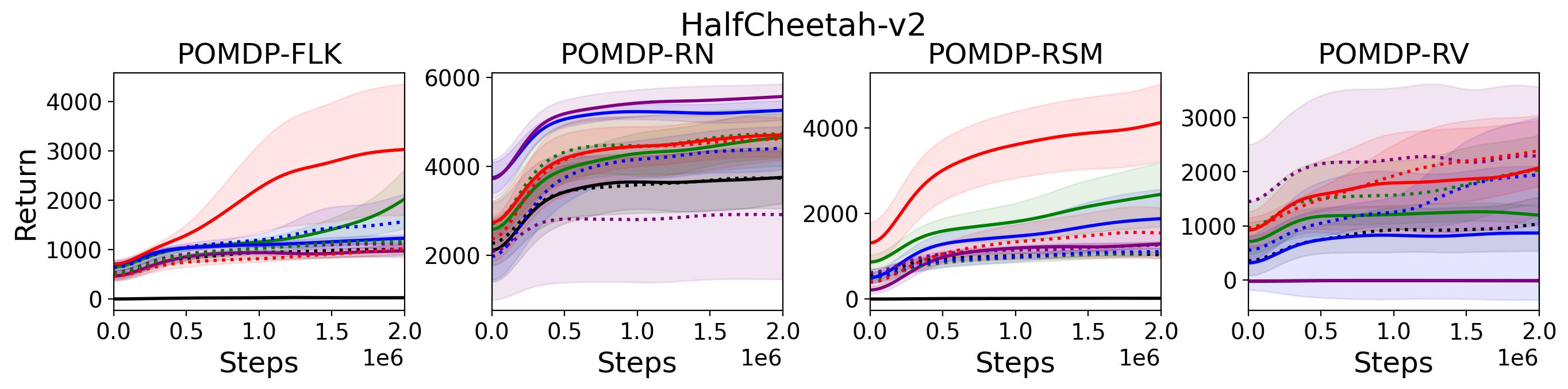
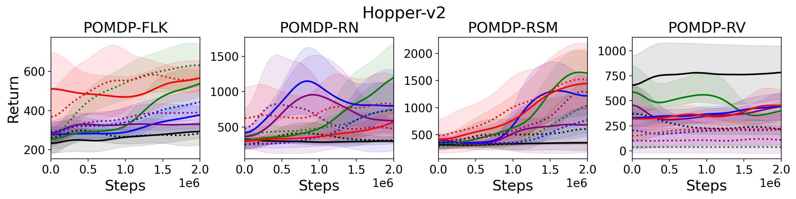
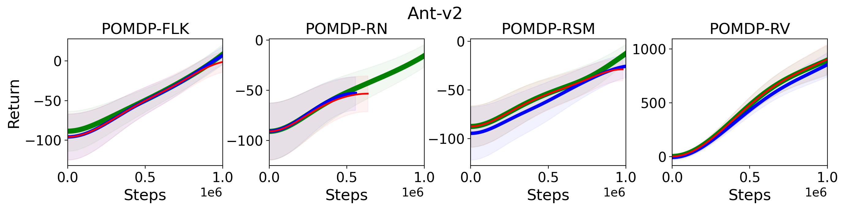
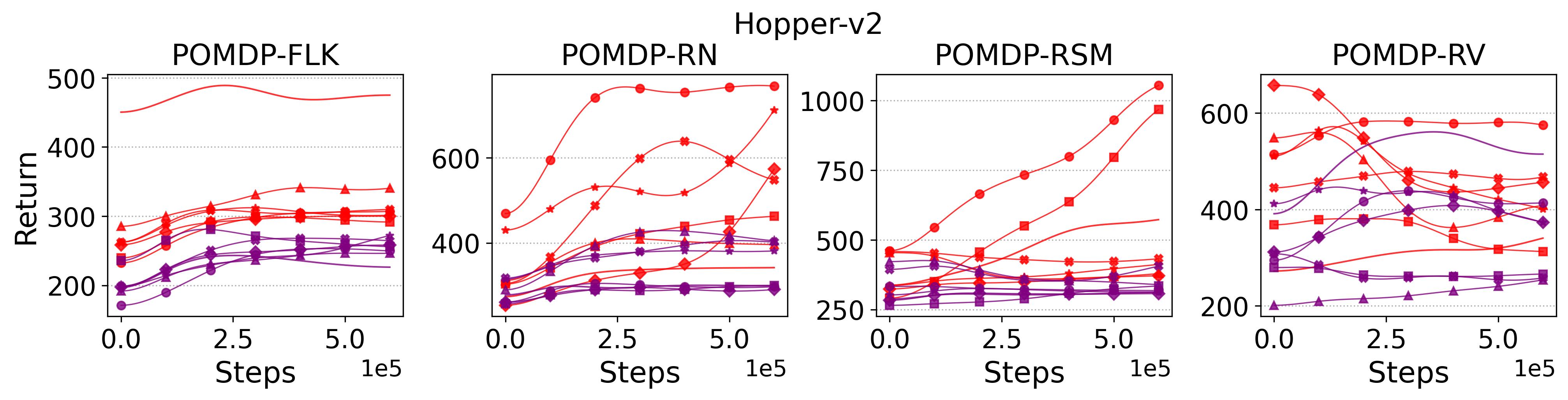
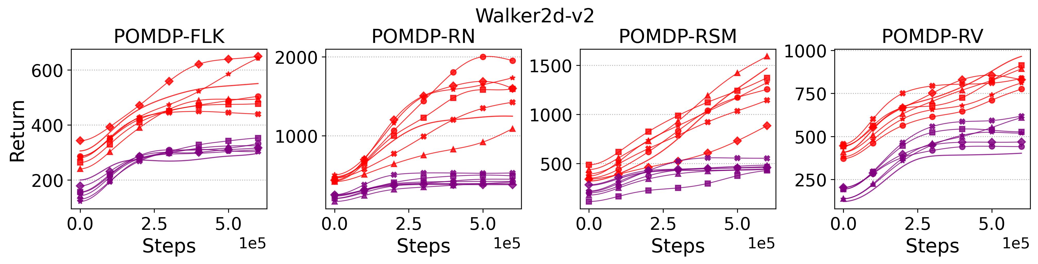
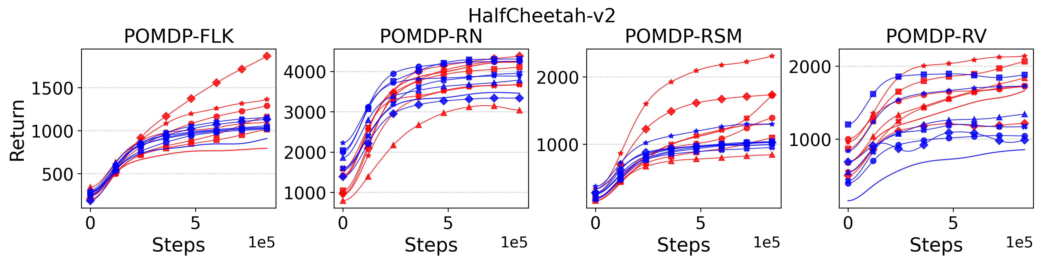
To investigate the generalization of the unexpected result introduced in the exemplar robot control problem in Section 4 and validate the Hypothesis 1 made in in Section 5, we run PPO, TD3 and SAC on both the MDP- and POMDP-versions of Ant-v2, HalfCheetah-v2, Hopper-v2, and Walker2D-v2. The results on each task are shown in Table 3333The corresponding learning curves can be found in Fig. 14 in Appendix A.3, and for better visualization, the average return over tasks listed in Table 3 are summarized in Table 4 and Fig. 4. It can be seen from Table 3 that on the MDP-version of the 4 tasks TD3 and SAC achieve better performance than PPO. However, on the 4 POMDP-versions of the 4 tasks, PPO outperforms TD3 and SAC on 11/16 tasks as highlighted in gray in Table 3. In addition, when moving from the MDP to the POMDP, PPO experiences mild performance decreases for most cases with two exceptions, i.e., Ant POMDP-RV and Hopper POMDP-RSM, where PPO even has improved performance as highlighted by in Table 3. While in case of Cheetah the difference is small and it could be argued that it is purely statistical noise and is thus insignificant, in Ant the difference is quite large. Following the hypothesis that PPO could incorporate temporal information, a potential explanation is that velocity is indirectly incorporated and probably additionally adding it to the observation can only make the observation space larger and introduce difficulty in finding an optimal policy. However, remarkably TD3 and SAC all encounter significant performance decrease with no exception. These findings are highly consistent with the Hypothesis 1, alerting researchers that applying state-of-the-art DRL algorithms directly to a task with partial observation may be problematic.
7.2 Exploring the Effect of Multi-step Bootstrapping
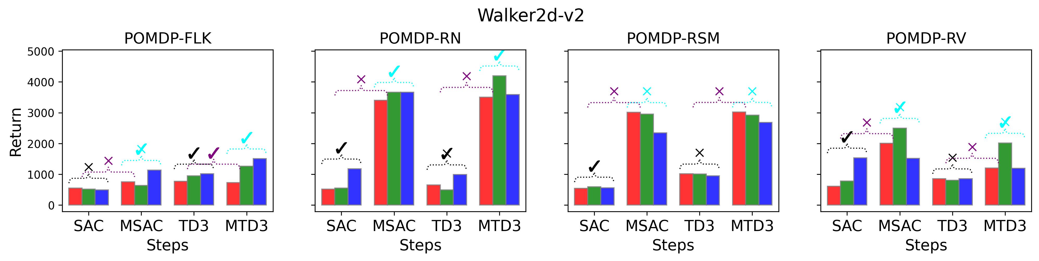
To test point (1) of Hypothesis 2, we compare the performance of MTD3(n) with TD3 and that of MSAC(n) with SAC in Table 3. As highlighted in red in Table 3, MTD3(5) significantly outperforms TD3 on 14/16 POMDP tasks, and similarly MSAC(5) significantly outperforms SAC on 15/16 POMDP tasks. More obvious performance improvement can be seen in Table 4 and Fig. 4 that when using multi-step bootstrapping TD3 and SAC achieve double performance on POMDPs compared to their vanilla version using 1-step bootstrapping. More interestingly, simply using multi-step bootstrapping with step size equal to 5 MTD3(5) and MSAC(5) achieves performance comparable to or even better than LSTM-TD3(5), which is specifically designed to deal with POMDPs. Nevertheless, this indicates that for some cases directly learning a good representation of the underlying state from a short experience trajectory as that in LSTM-TD3(5) is more effective than relying on multi-step bootstrapping to pass some temporal information.
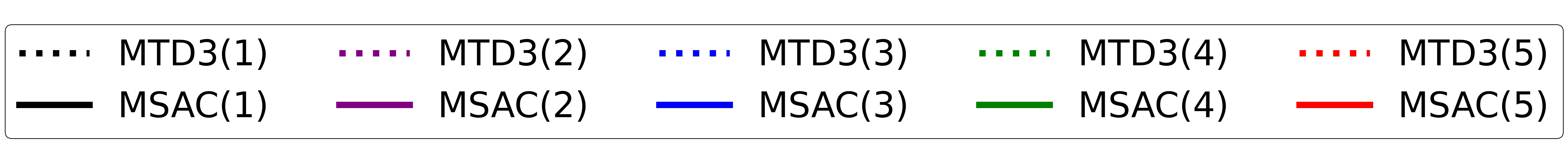
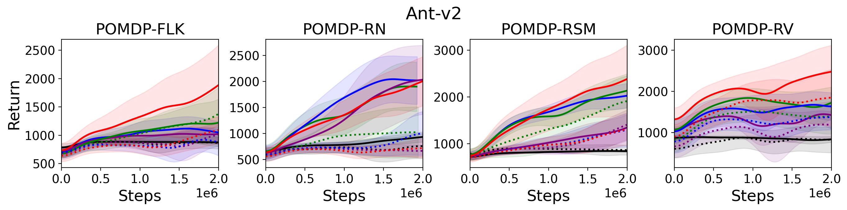
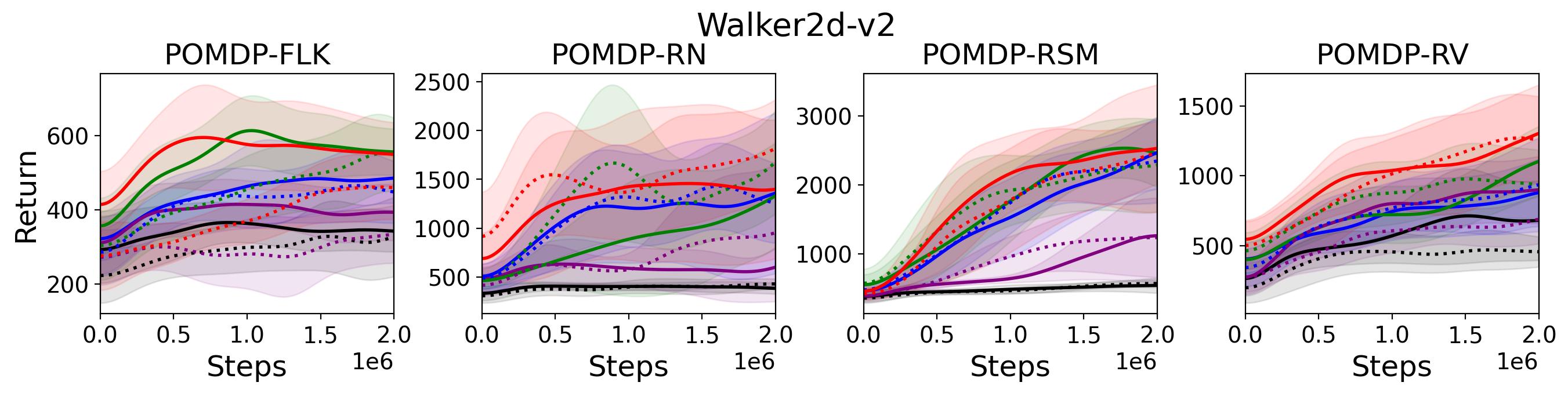
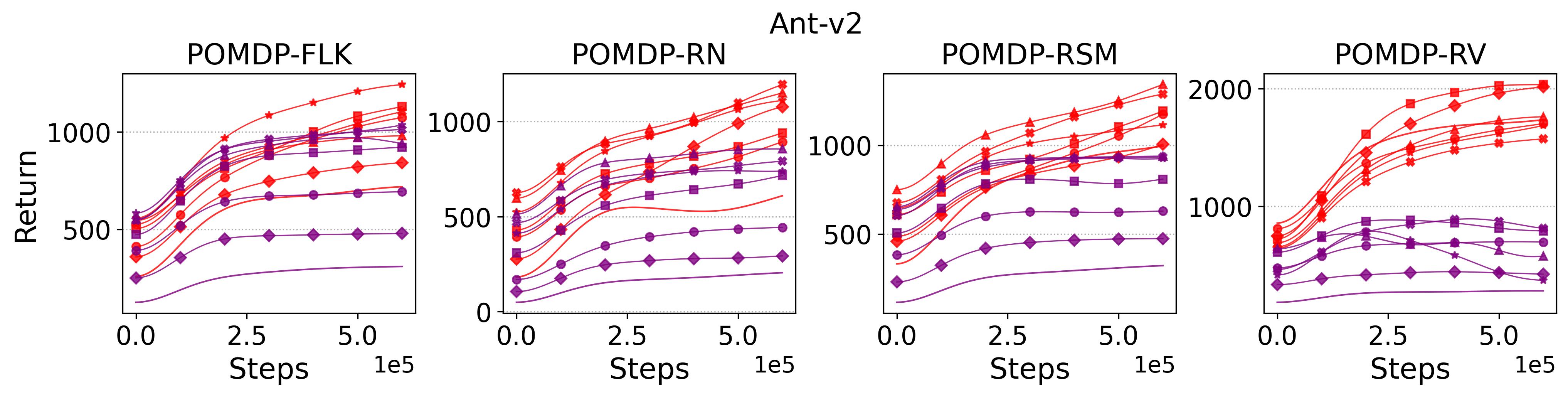
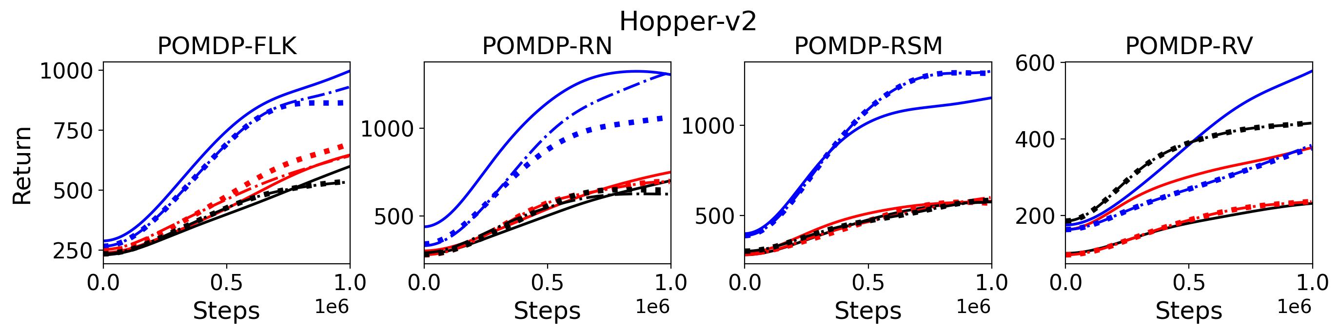
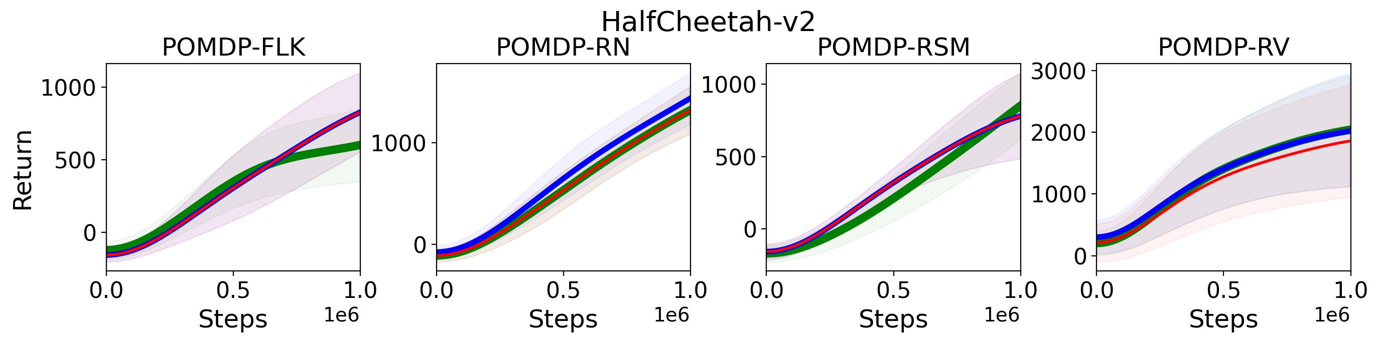
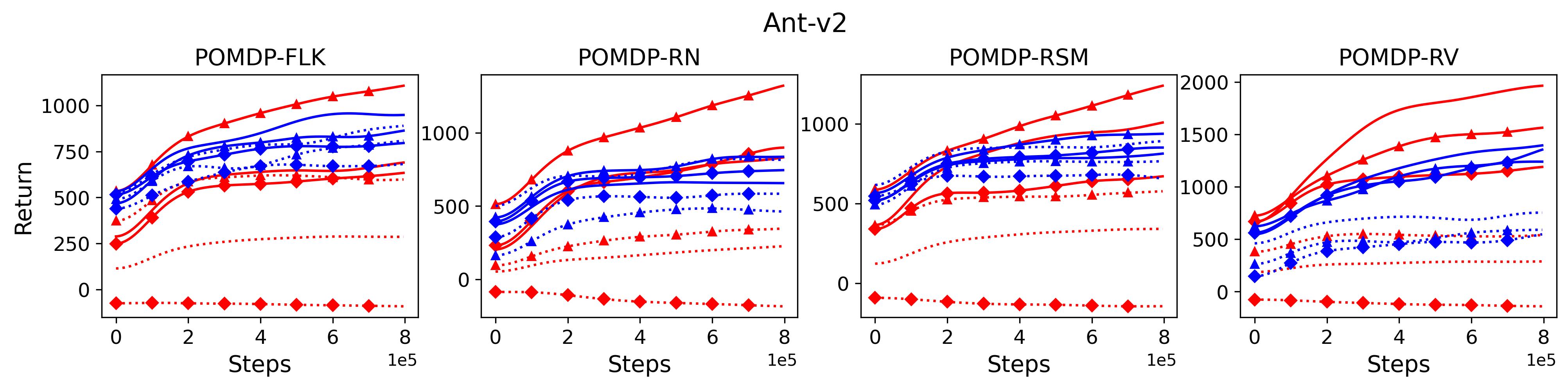
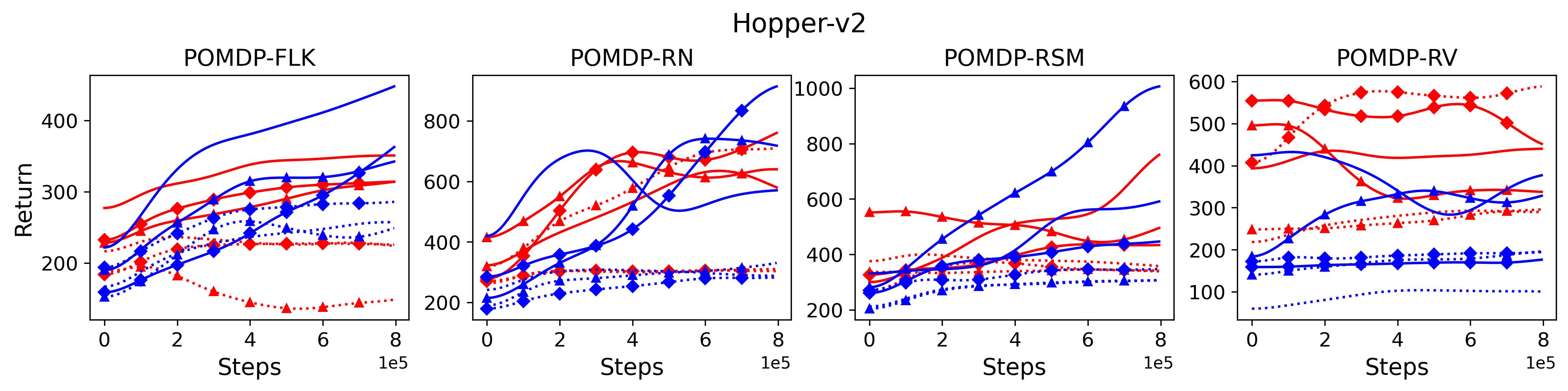
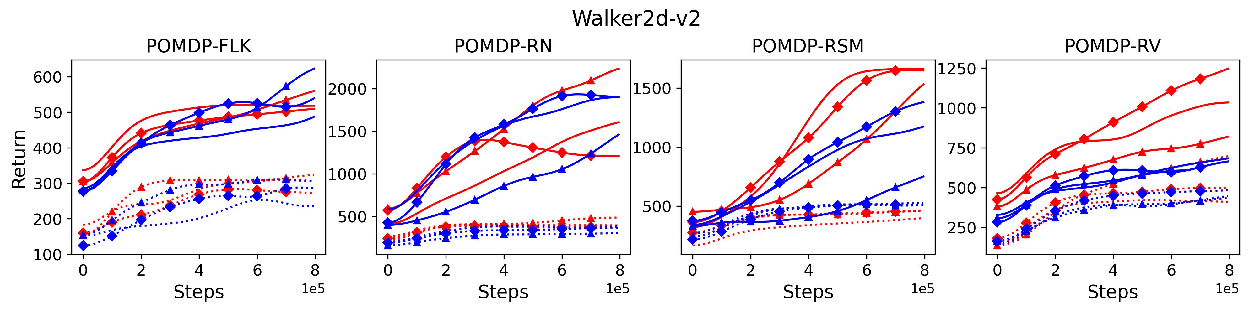
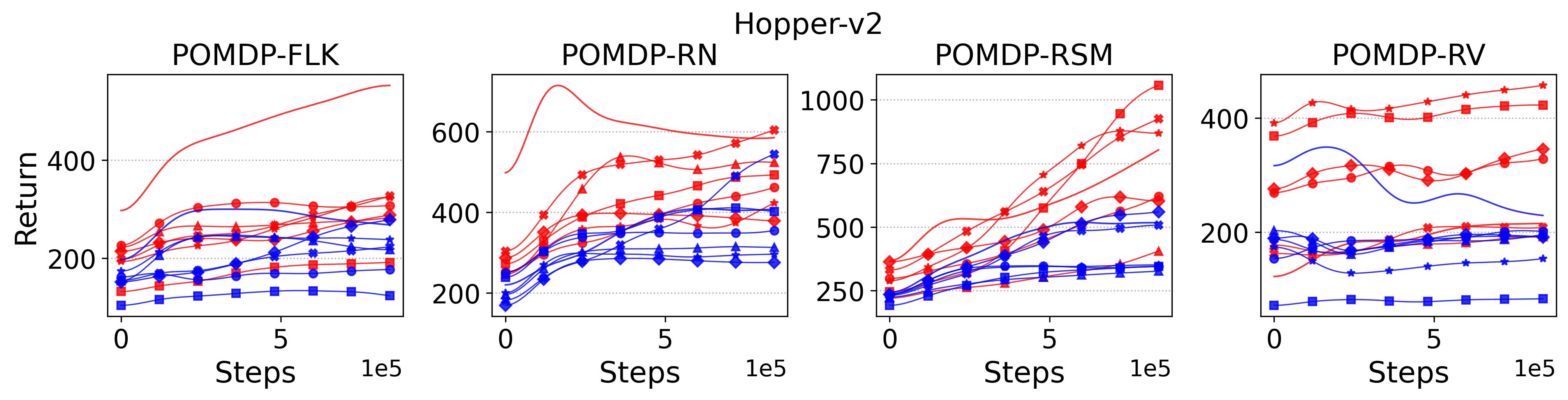
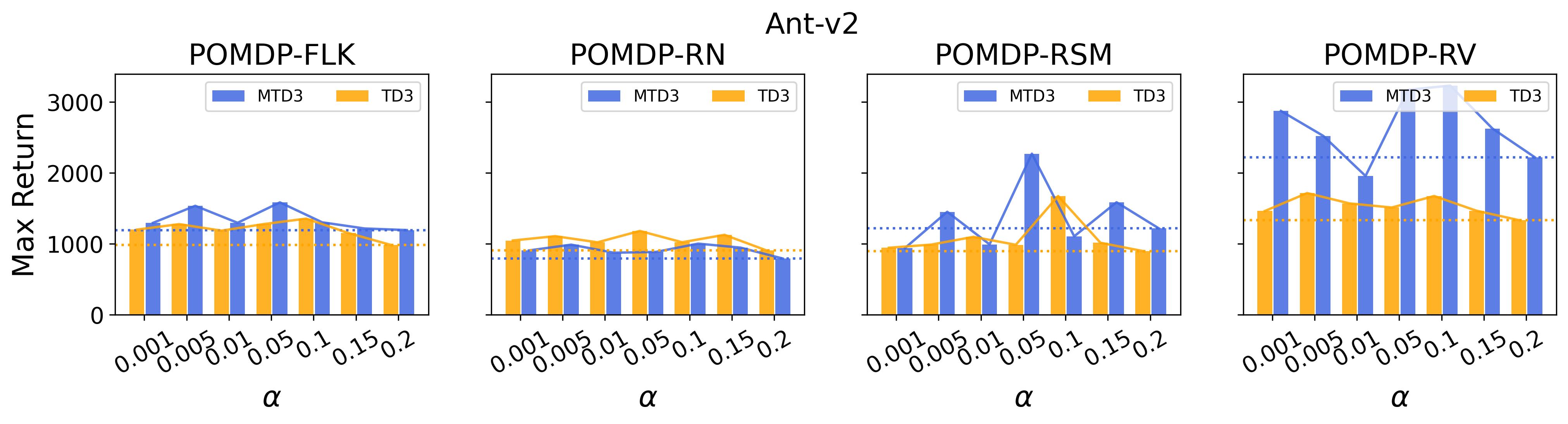
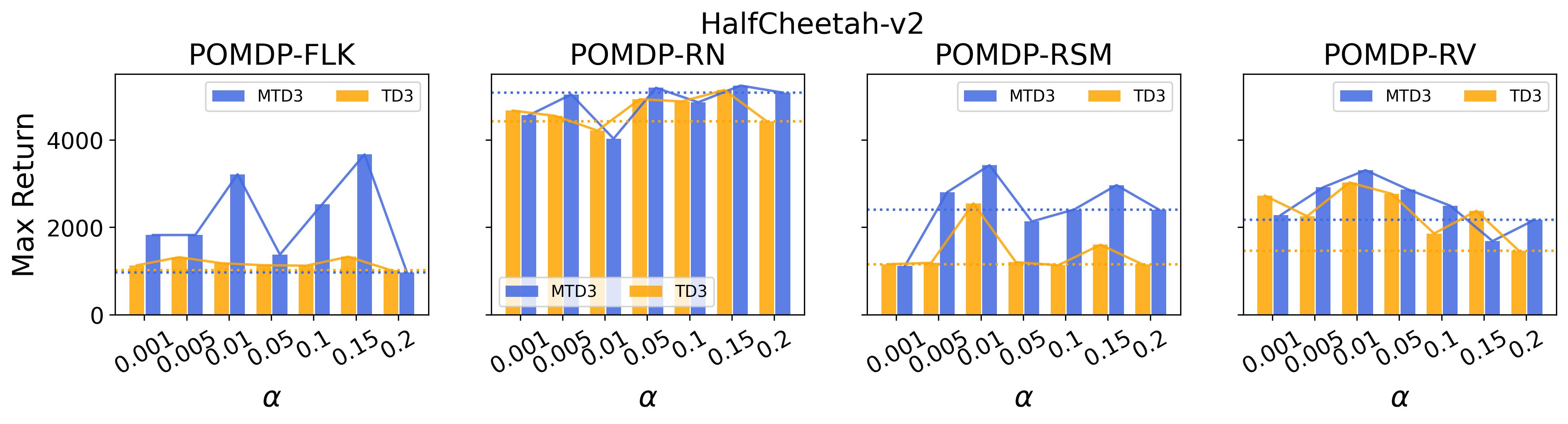
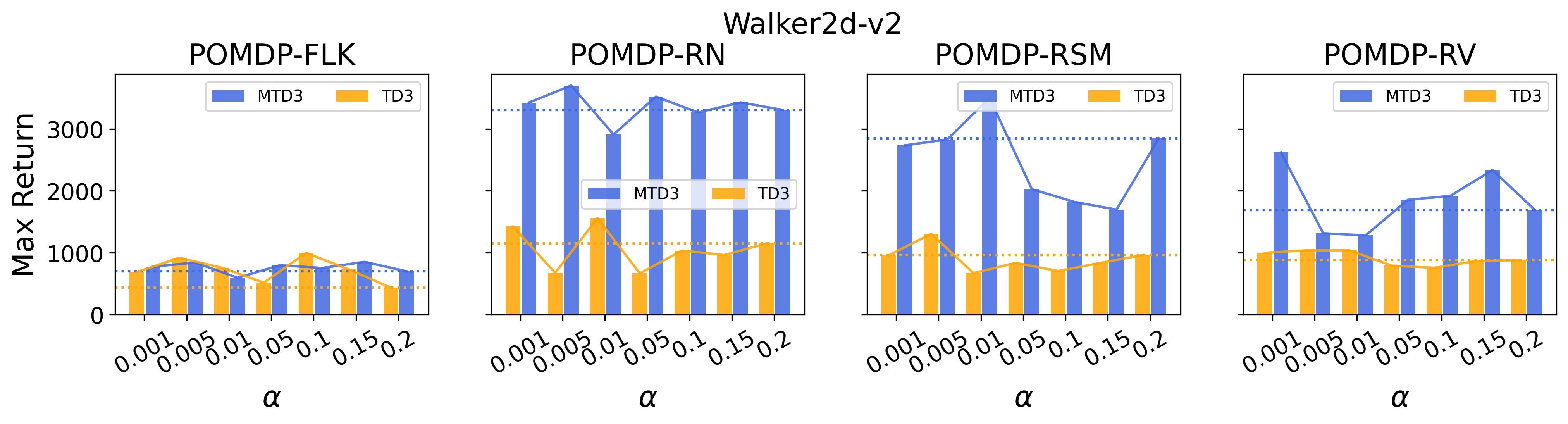
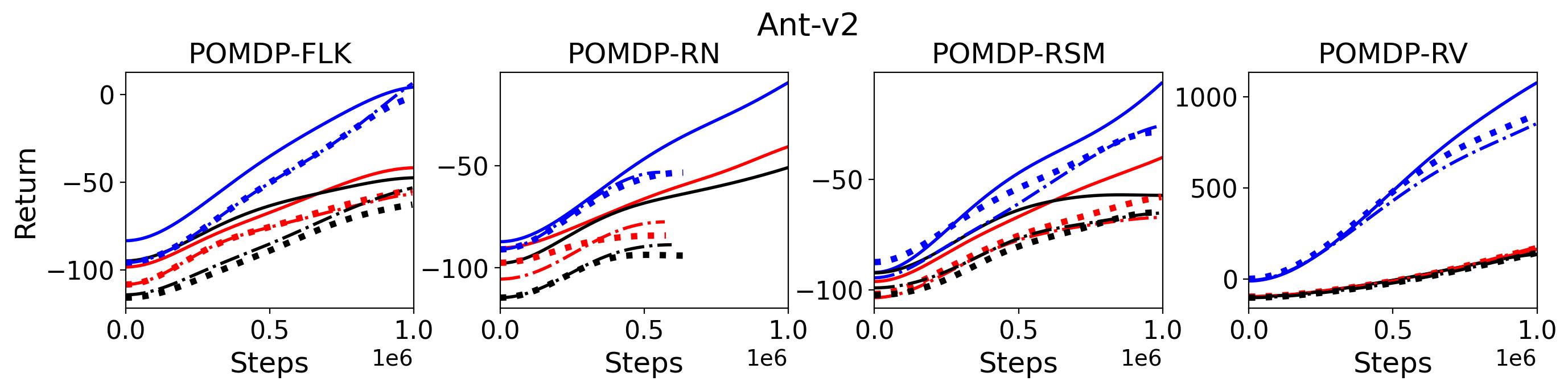
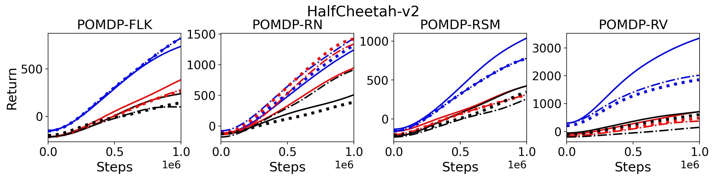
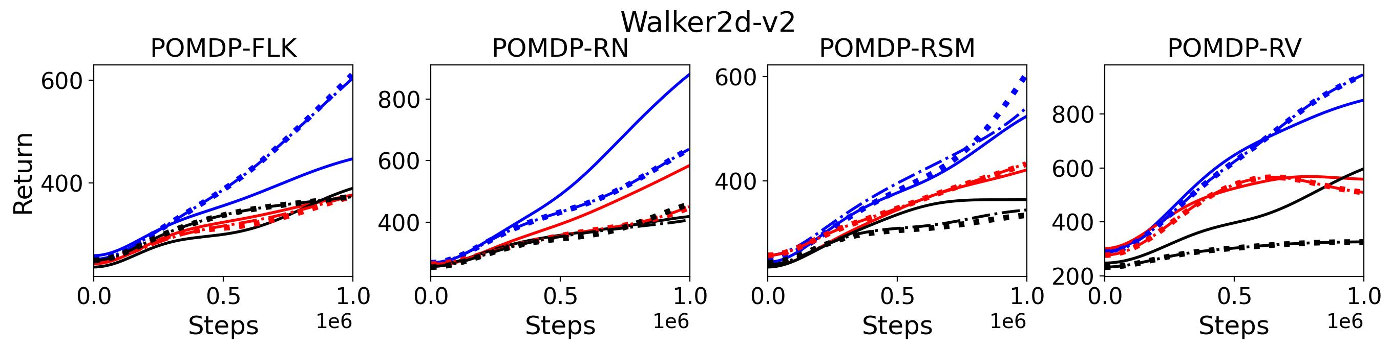
To investigate how the multi-step size affects the performance of MTD3() and MSAC(), Fig. 5 shows the average learning curves of MTD3() and MSAC() with different multi-step sizes . When these reduce to TD3 and SAC, respectively444More results on other tasks can be found in Fig. 15 in Appendix A.3.. It can be seen from Fig. 5 that simply increasing by a few steps increases performance dramatically over the case with limited extra computational cost. For the we tested, shows the best performance on most tasks. Table 5 summarizes the best performance of MTD3() and MSAC() with different multi-step sizes , where we specifically compare with for MTD3() and MSAC() on the 16 POMDP tasks. It can be seen that simply increasing step size from 1 to 2, results in an MTD3(2) performance improvement on 11/16 tasks, while MSAC(2) improves its performance on 14/16 tasks. With the larger step size used, both MTD3() and MSAC() get much better performance. These findings all support (1) of Hypothesis 2 and reveal the benefit of multi-step bootstrapping when handling POMDPs.
| MTD3(n) | MSAC(n) | ||||||
| 11/16 | 13/16 | 13/16 | 14/16 | 14/16 | 13/16 | 14/16 | 16/16 |
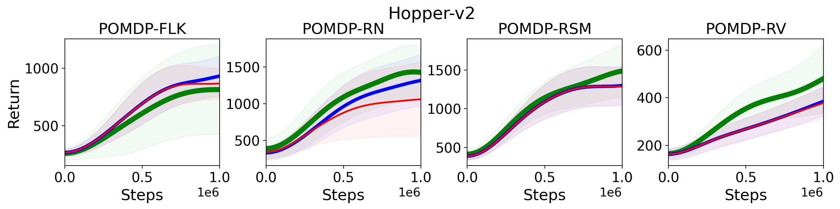
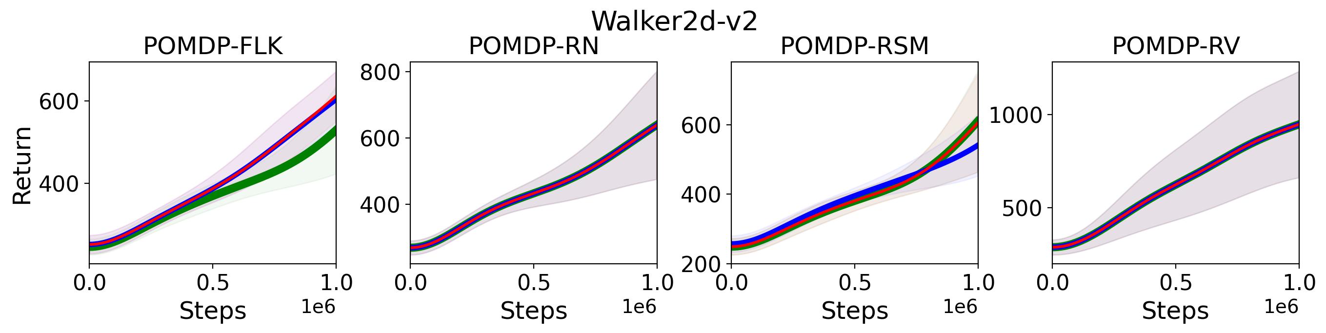
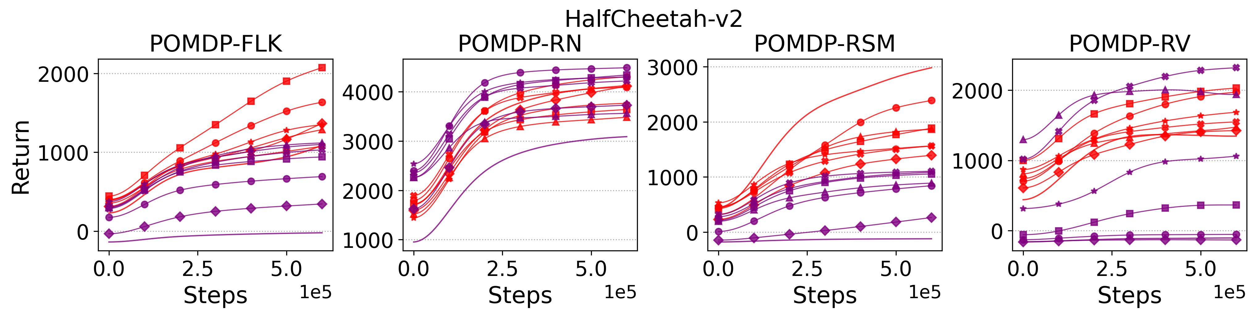
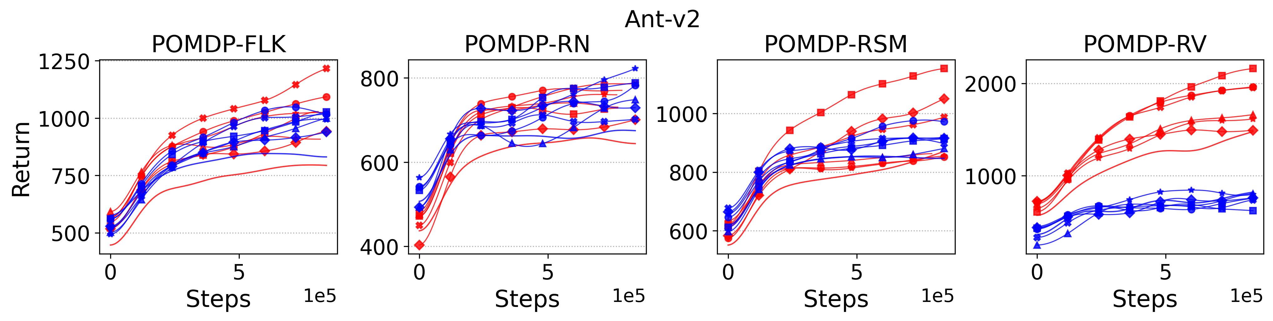
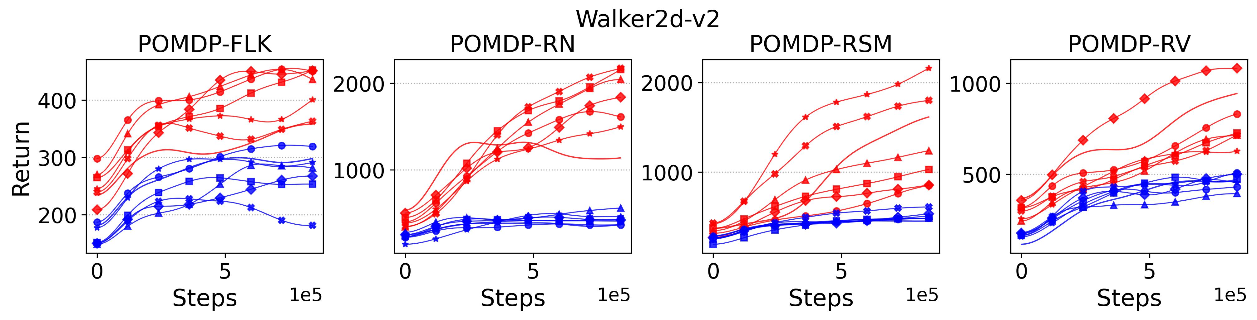
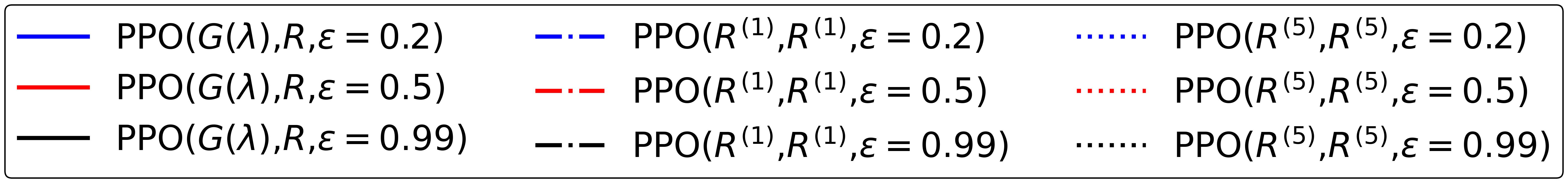
To validate (2) of the Hypothesis 2, we replace the -return used to calculate generalized advantage estimate and Monte-Carlo return used to update state-value function with -step bootstrapped return for both advantage estimate and policy update, where results for PPO(,) with is compared with the original PPO(, ) in Fig. 6 555More results on other tasks can be found in Fig. 16 in Appendix A.3.. As shown in this figure, there is no clear difference among PPO(, ), PPO(,) and PPO(,). For example, on Walker2d-v2 POMDP-RN and POMDP-RV the performance of these three variances of PPO almost perfectly overlapped. Therefore, the results shown in Fig. 6 rejects the (2) of the Hypothesis 2
To summarize, the results shown in this section support (1) of Hypothesis 2 that multi-step versions of TD3 and SAC, i.e., MTD3(n) and MSAC(n), with significantly improve their performance compared to their vanilla versions, but (1) of Hypothesis 2 is rejected by our results that replacing the -return and Monte-Carlo return with 1-step bootstrapped return does not cause the performance decrease for PPO.
7.3 Observation and Action Coverage of Policy With One-step or Multi-step Bootstrapping
In Section 7.2, we demonstrated the effect of multi-step bootstrapping on improving TD3’s performance on POMDPs in Fig. 5. The measurement used in that section is the accumulated reward, i.e. return. In this section, we will have a look at the difference in terms of observation and action coverage between TD3 and MTD3(5) leveraging dimensionality reduction technology to get more insights on the difference in the policies induced from one-step and multi-step bootstrapping. Specifically, we will try to embed the high-dimensional observation and action space into 2D space for visualization.
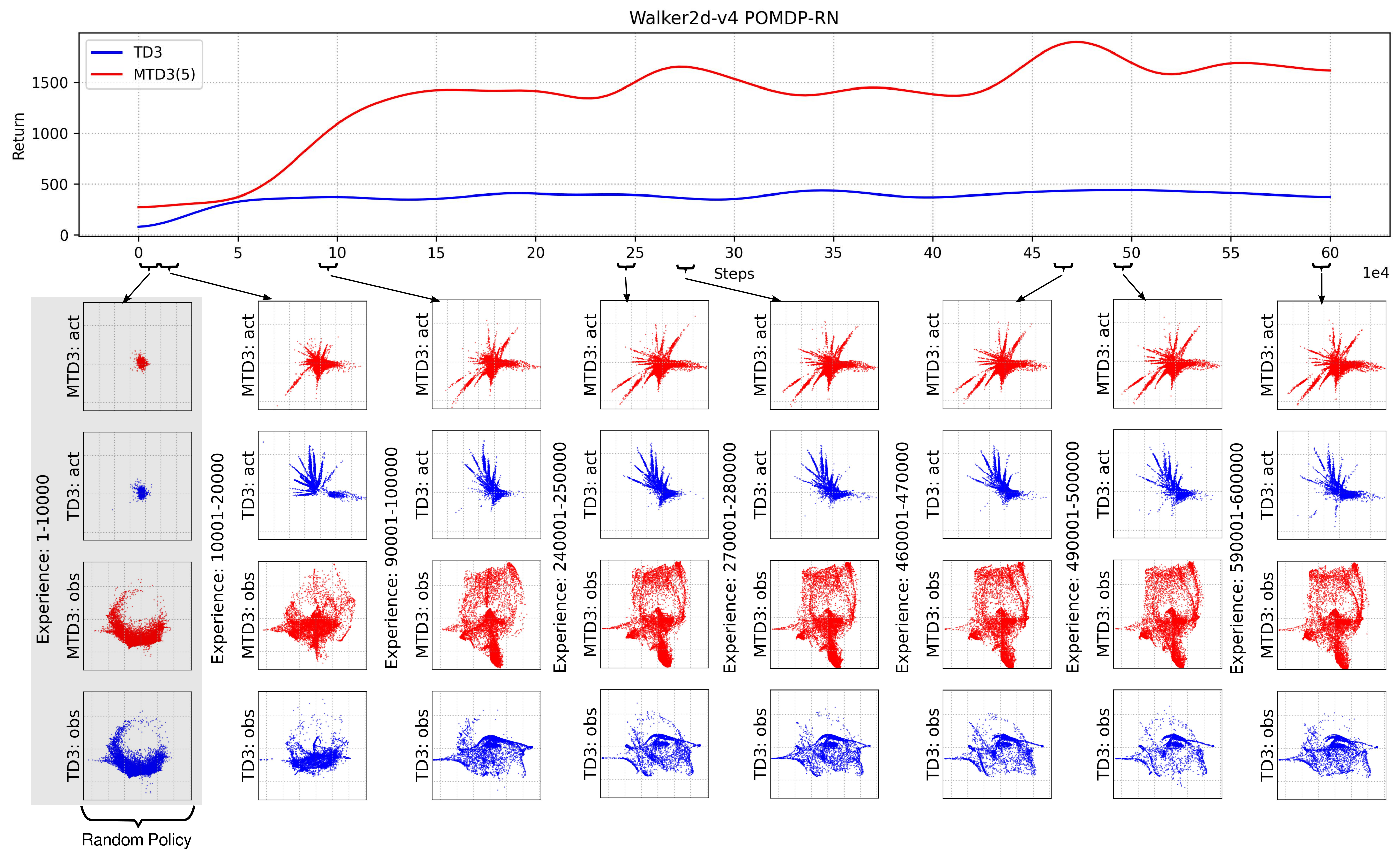
Fig. 7 compares the observation coverage of the policy learned by TD3 and MTD3(5) on Walker2d-v4 POMDP-RN, where each of the bottom panels shows 10000 observations and the actions taken by TD3 and MTD3(5) in these observations. In order to compare, we first separately combine the observations and actions collected by TD3 and MTD3(5) and then embed them into 2D using TriMap(Amid and Warmuth, 2019), where TriMap is used for dimensionality reduction because it is good at maintaining the relative distances of the clusters compared to other methods, e.g., T-SNE (Van der Maaten and Hinton, 2008). Because for both TD3 and MTD3(5) the first 10000 steps are driven by a random policy, the observation and action coverage of TD3 and MTD3(5) are very similar, as shown in the first column of Fig. 7. However, once the learned policy is used to take actions, there is an immediate observation and action coverage difference between TD3 and MTD3(5) as shown in the 2nd column of the figure where the experiences from time step 10001 to 20000 are plotted. As the learning continuing, not only the TD3 and MTD3 have different observation and action coverage for time step from 90001 to 100000, they also have different coverage compared to that from time step 10001 to 20000. This indicates the policies of TD3 and MTD3(5) are evolving to different local optimal. From the last few columns of Fig. 7, we can see from the observation and action coverage plots the policies of TD3 and MTD3(5) are relatively stable after 150000 steps, and there is a distinct difference between TD3 and MTD3(5), which also matches the difference in the performance of the policies.
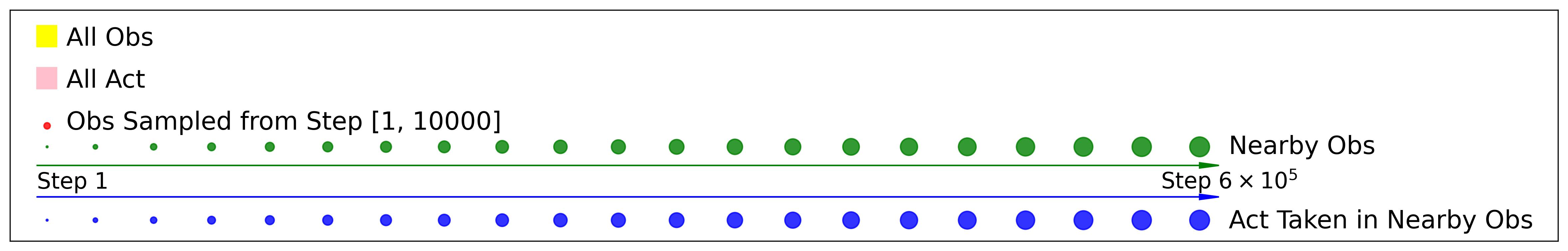
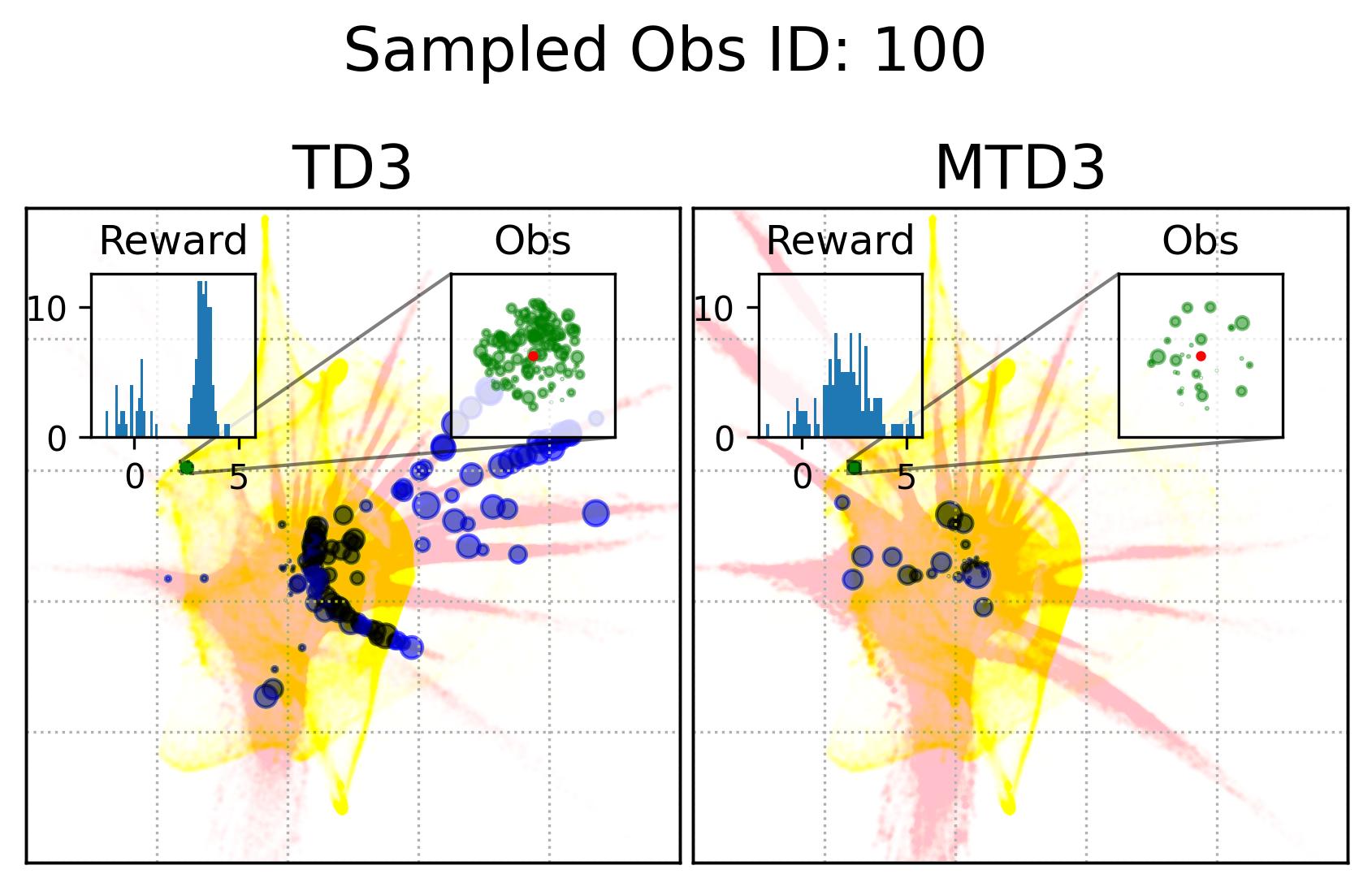
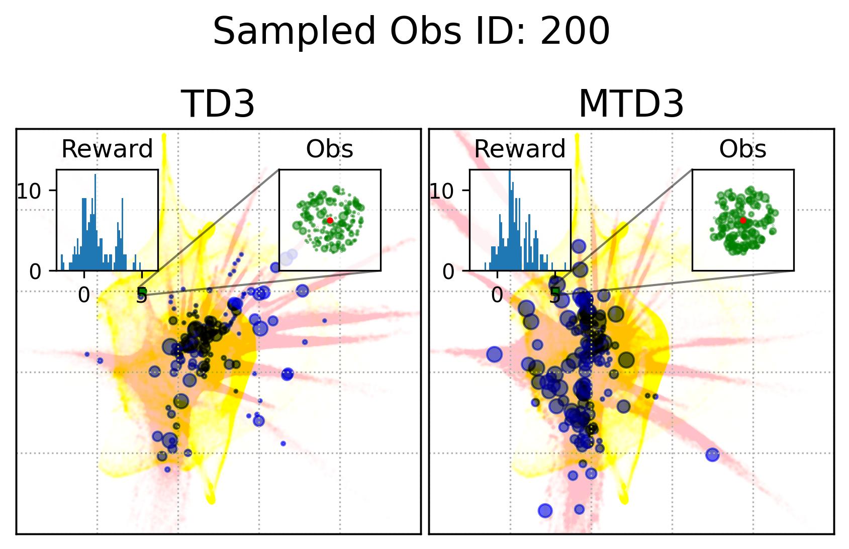
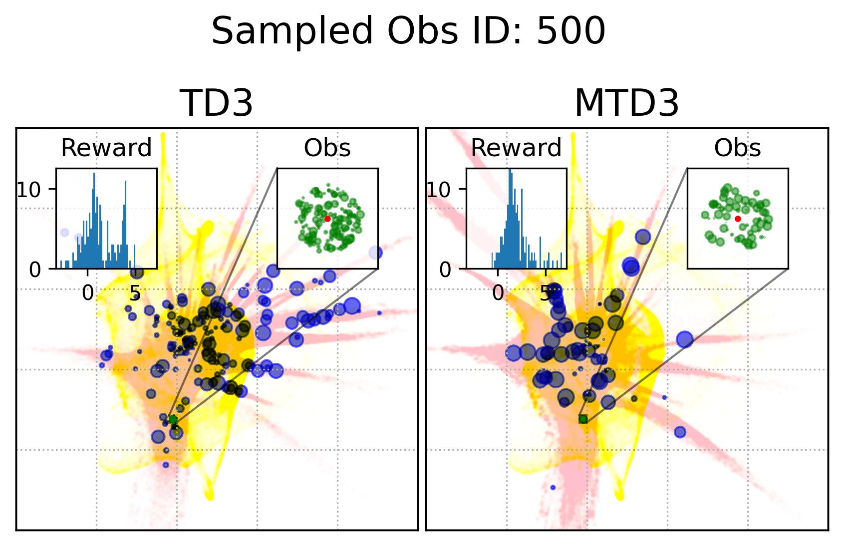
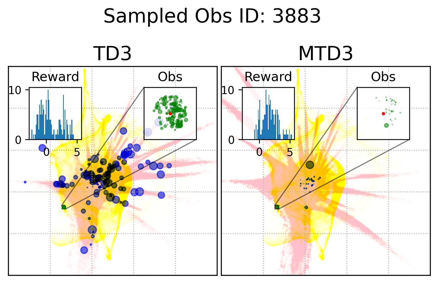
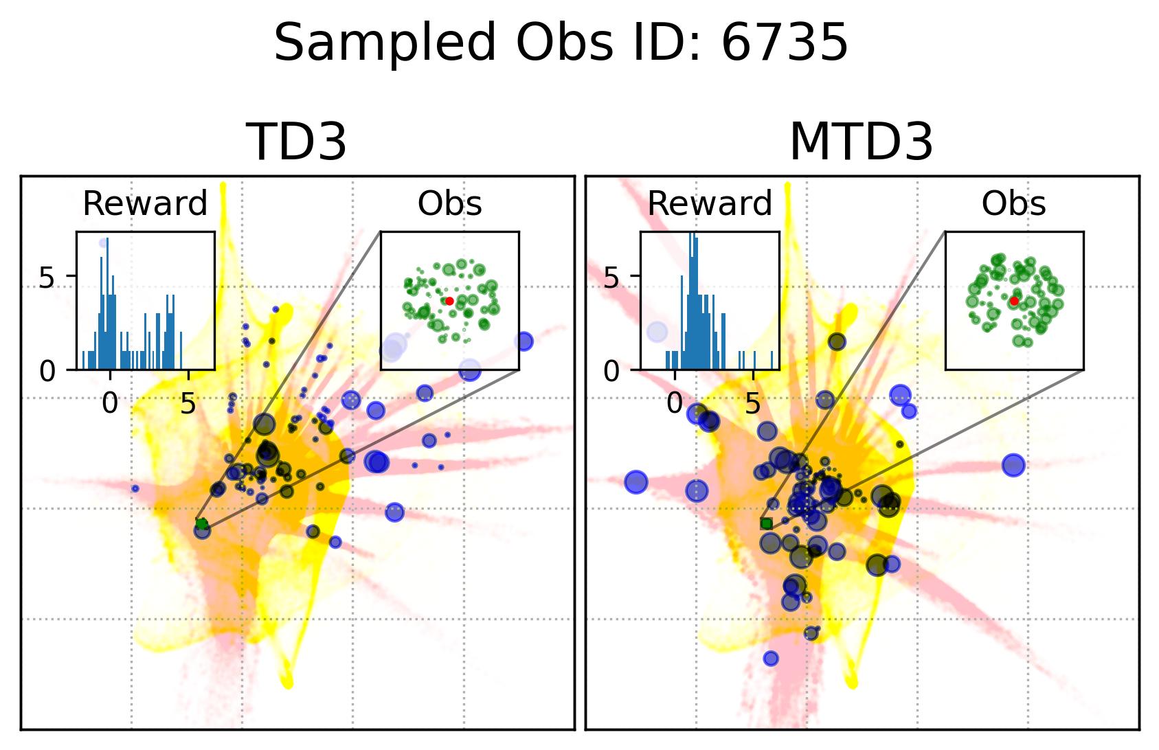
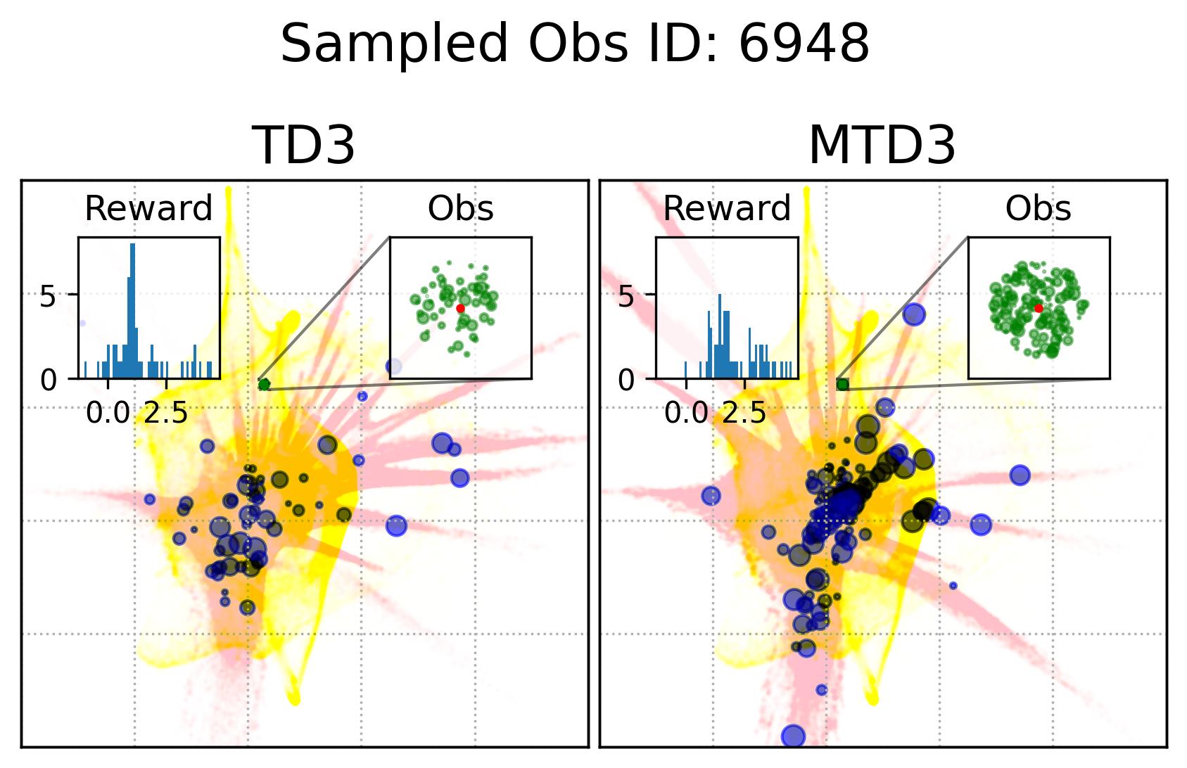
Fig. 7 shows the observation and action coverage difference between TD3 and MTD3(5) from a broader perspective where the observations and actions within one period of 10000 time-steps are compared to another period. To have a closer look at their different at a specific observation, Fig. 8 shows the actions taken in observations that are nearby an observation sampled from the first 10000 experiences. The nearby observations of an observation is defined as where the and are embedded 2D observations whose value range for each dimension is . The neighbour observations (the green dots) of a sampled observation (the red dot) are better visualized in the inset of each panel. The corresponding actions taken in these neighbour observations are represented by the blue dots whose sizes are used to reflect the happening time of these actions where the more recent the action was taken the bigger the dot will be, as indicated by the legend of Fig. 8. In addition, to give the readers a sense of where the sampled observation, the neighbours of the sampled observation, and the action taken in these neighbour are relative to the whole embedded observations and actions, Fig. 8 also show the whole embedded observations in yellow and whole embedded actions in pink. To show how good these actions are, the histogram of the reward of taking these actions in the neighbour observations is shown in each panel as well. The 1st distinct difference between TD3 and MTD3(5) that can be drawn from Fig. 8 is that the actions taken by MTD3(5) in the neighbour observations are quiet different from that taken by TD3, which indicates the policy difference, and the actions taken by MTD3(5) correspond to higher rewards compared to that of TD3 as shown in the inset titled “Reward”. However, what is common between TD3 and MTD3(5) is that even though the neighbour observations are tightly close to each other, the actions taken in these observations are not so close to each other. This can be because the small difference in the observation may cause a big difference in optimal action. Another explanation could be the relative distances of actions are not well maintained by TriMap. It is also interesting to see that some observations are frequently encountered by TD3 but are rarely observed in MTD3(5), especially at the newest interactions, e.g., the 1st column of the 1st and the 2nd row, which is also an indicator of the difference between TD3 and MTD3(5) and showing that MTD3(5) learns a policy to avoid these observations whereas TD3 is stuck in a local optimal that cannot escape from it.
As a summary, the results shown in this section demonstrate the difference in the policies derived from one-step and multi-step, specifically 5-step, bootstrapping for TD3, as a measurement to reflect the difference in learning performance, namely accumulated reward. We know that the policy of TD3 and MTD3 is derived from the action-value function, so this means essentially multi-step bootstrapping leads to a better value function than one-step bootstrapping that is robuster to partial observation of the underlying state. However, it is still unclear why simply replacing the one-step bootstrapping with a multi-step bootstrapping can make such a difference in the performance of DRL algorithms, i.e., TD3 and SAC, on POMDPs, especially given that the (2) of the Hypothesis 2 is rejected in Section 7.2.
7.4 Effect of Accumulated Reward
To validate Hypothesis 3, results on environment using average reward (Eq. 11) and summation reward (Eq. 12) over consecutive rewards are compared with that on environment using the original reward. Table 6 shows the aggregated results on the 16 POMDPs666The results on each task can be found in Appendix A.3.3.. It shows that the proportion of the 16 POMDPs that the performance of an algorithm (right side of ) on environment using accumulated reward, i.e., or defined in Eq. 11 and Eq. 12 respectively, is better than that of another algorithm (left side of ) on environment using original reward . Over all comparisons, only two cases, i.e., and , experience majority (over 50% of tasks) performance improvement, while for other cases there is a performance decrease for most tasks. What particularly evident is TD3 and SAC on environment using accumulated reward can not achieve comparable performance of MTD3(5) and MSAC(5) on environment using the original reward, as highlighted in gray in Table 6.
The results shown here reject Hypothesis 3, which are: (1) the performance of TD3 and SAC on environment using accumulated reward is not consistently improved compared to their performance on environment using the original reward, and (2) for cases there are performance improvement, the performance improving scale is not comparable to that of algorithms using multi-step bootstrapping. This hints the mechanism underlying the performance improvement and robustness to POMDP of algorithms using multi-step bootstrapping, e.g., MTD3 and MSAC, is more complicated and cannot be simply explained by the intuition that multi-step rewards can passing temporal information. Therefore, in the following section we will investigate if the Unexpected Result is related to the Diff 2, i.e., exploration strategy.
| Comparison | Proportion | |
| TD3 TD3 | 6/16 | 5/16 |
| SAC SAC | 5/16 | 14/16 |
| MTD3(5) TD3 | 2/16 | 1/16 |
| MSAC(5) SAC | 0/16 | 0/16 |
| MTD3(5) MTD3(5) | 5/16 | 9/16 |
| MSAC(5) MSAC(5) | 4/16 | 5/16 |
| Note: indicates either or is used. | ||


7.5 Results on Investigating the Effect of the Exploration Strategies
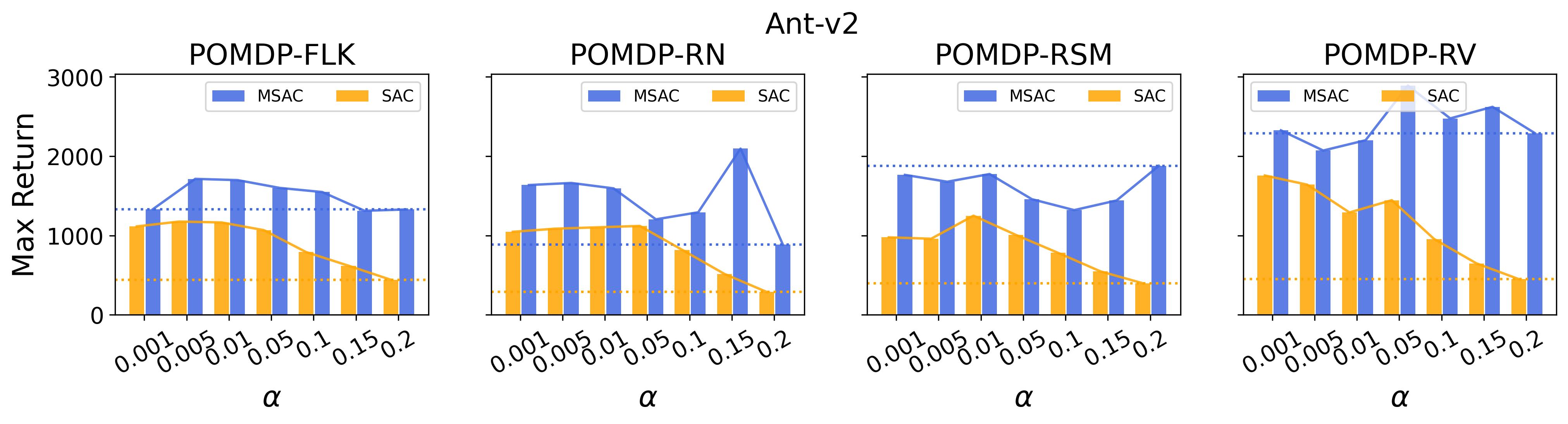
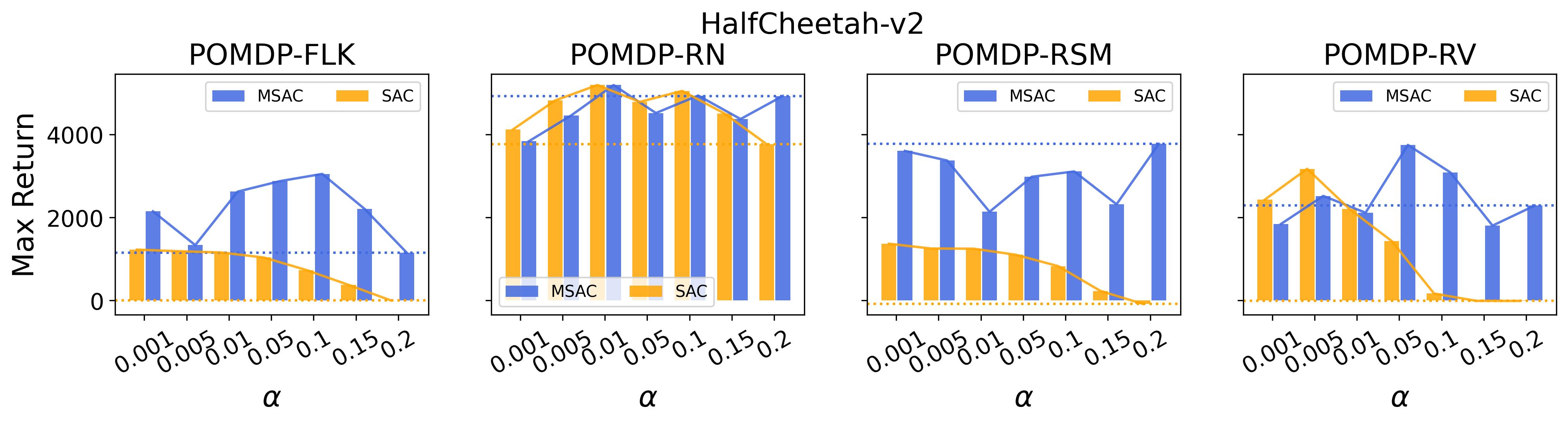
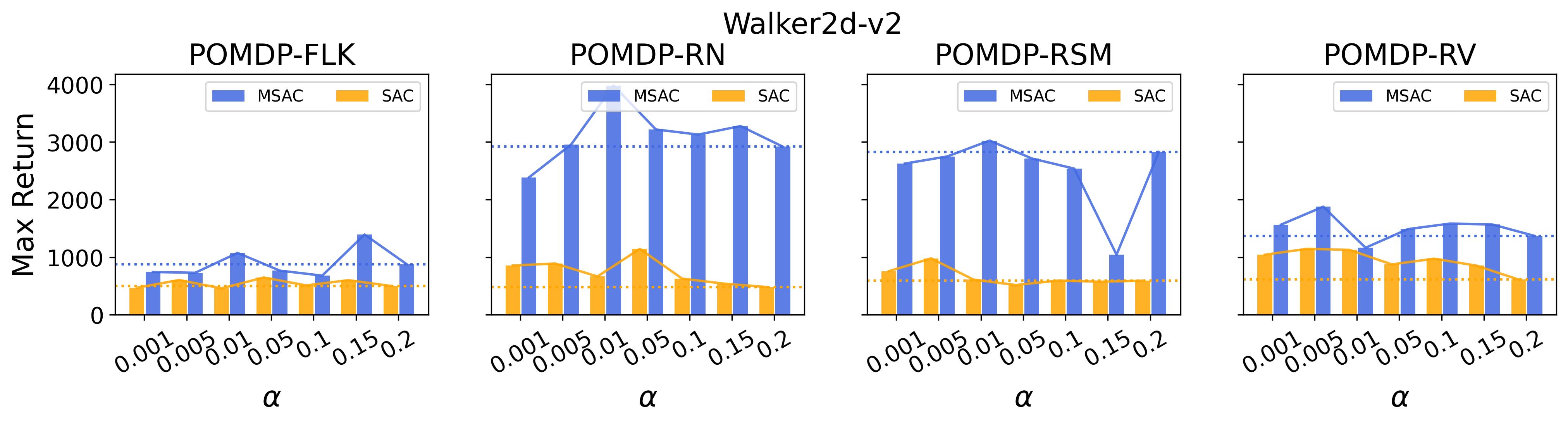
In the (1) of Hypothesis 4 we assume less exploratory strategy can make TD3 and SAC robuster to POMDP, so to validate this, we investigate SAC with and TD3 with . For both and , the larger the parameter is, the wilder the exploration will be. The commonly used default value for and are 0.2 and 0.1, respectively, as that for the results reported in Table 3. Fig. 9 shows results of SAC and MSAC(5), while Fig. 10 shows results of TD3 and MTD3(5)777More results can be found in Appendix A.3.4.. Firstly, let us have a look at SAC and MSAC(5). As shown in Fig. 9, overall reducing the exploration can not make SAC consistently beat MSAC(5), even though there are exceptions, e.g., on HalfCheetah POMDP-RV SAC with has better performance than MSAC(5) with . Nevertheless, for some cases, e.g., the POMDP variants of Ant-v2 and HalfCheetah-v2, reducing the exploration of SAC indeed allows it to achieve better performance, while for MSAC(5) reducing the exploration seems having less effect than that on SAC. Secondly, similar overall observations can be found for TD3 and MTD3(5) as shown in Fig. 10 that for most tasks reducing TD3’s exploration cannot achieve comparable performance of MTD3(5), especially for Walker2d-v2. However, we can see the different effect of reducing exploration for TD3 and SAC on Ant-v2, where SAC can get significant performance improvement from less exploratory policy while TD3 cannot. To summarize, it is not consistently observed that reducing the exploration in TD3 and SAC can make them robuster to POMDP, so the (1) of Hypothesis 4 cannot be supported by our results. However, what is clear from these results is that for TD3 and SAC multi-step bootstrapping can help more than less exploratory strategy in terms of improving their performance on POMDPs.
In the (2) of Hypothesis 4 we assume wilder exploration strategy can make PPO vulnerable to POMDP, so to validate this, we investigate PPO with , where is the commonly used default value for PPO. The results are presented in Fig. 11, where we also show results on PPO(, , ), i.e., the revised PPO using -step bootstrapped return for both advantage estimate and state-value function update. In the figure, the blue-, red- and black-colored lines correspond to low, mediate, and large exploration, respectively. To save space, we only show results on Hopper-v2, but the results on Ant-v2, HalfCheetah-v2 and Walker2d-v2 are very similar and can be found in Fig. 23 in Appendix A.3.4. Since Section 7.2 has discussed the effect of the multi-step bootstrapping of PPO in the Fig. 6, we will mainly consider the effect of exploration strategy here. It can be seen from the figure that for both the original PPO(, , ) and the variants of PPO(, , ), increasing the exploration leads to worse performance for most cases, which strongly supports the (2) of Hypothesis 4.
As a summary for the validation of Hypothesis 4, the (1) of Hypothesis 4 is not supported by our experiment results as there is no consistent trend can be found that reducing the exploration in TD3 and SAC makes them robuster to POMDPs, whereas the (2) of Hypothesis 4 is strongly supported by our results that on most POMDPs increasing the exploration of PPO makes it vulnerable to POMDPs. These results reveal that the Unexpected Result cannot be explained by the Diff 2 too.
8 Discussion
The Hypothesis 1 on the generalization of the Unexpected Result found in Section 4 is validated by the similar results on other standard benchmarks presented in Section 7.1. This strongly indicates the unexpected result will apply to other domains. As a concrete example, Meng (2023) also find similar unexpected result when applying the state-of-art DRL algorithms to a Living Architecture System, an architectural-scale interactive system with hundreds of actuators and sensors embedded in, where the initial observation space design failed to capture temporal information and leading to a POMDP, and the researchers have to use aggregated information within an observation windows to tackle the unexpected result and get the Expected Result . This finding on the generalization of the Unexpected Result forms one of the key contributions made by this work and can provide a meaningful guide to researchers when a novel application faces the similar unexpected result.
Even though this work cannot provide a clear explanation on the Unexpected Result , this work proposes three hypotheses, namely Hypothesis 2, 3 and 4, based on our analysis on the two key differences, Diff 1 and 2, between PPO and TD3 and SAC, and experimentally validate these hypotheses in order to provide more insights to understand the Unexpected Result . The authors believe the experimental findings in this work can provide some useful information for the future research on theoretically explaining why the unexpected result happens, which is another key contribution of this work.
More specifically, based on Diff 1 related to multi-step bootstrapping, we first proposes Hypothesis 2. The results in Section 7.2 validate that using multi-step bootstrapping in TD3 and SAC, which lead to MTD3 and MSAC, significantly improves the performance of TD3 and SAC on the POMDPs, which strongly supports the (1) of the Hypothesis 2. Nevertheless, the result on PPO, whose -return and Monte-Carlo return are replaced with one-step bootstrapped state-value function, does not experience performance decrease and rejects the (2) of the Hypothesis 2. This finding is particularly interesting, as the experimental results clearly indicate multi-step bootstrapping can significantly improve TD3 and SAC’s performance on POMDPs compared to one-step bootstrapping but for PPO using one-step bootstrapping seems does not affect anything. Also based on Diff 1, Hypothesis 3 tries to replace the original reward with an accumulated reward and expects this can generate similar performance boost to that of using multi-step bootstrapping for TD3 and SAC as validated in Hypothesis 2. The results in Section 7.4 reject Hypothesis 3 that using accumulated reward cannot consistently improve TD3 and SAC’s performance not saying achieving comparable performance to MTD3 and MSAC.
Based on Diff 2, Hypothesis 4 assume the Expected Result is caused by the less exploratory policy of PPO. The (1) of Hypothesis 4 cannot be supported by our results in Section 6.0.3, because no consistent performance improvement is observed when changing the exploration level in TD3 and SAC, even though on some tasks it shows that having a lower exploration level can help to get a better performance. On the contrary, the results show that increasing the exploration level of PPO does make it vulnerable to POMDP, which can be seen as a strong support of the (2) of Hypothesis 4.
| Hypothesis | H 1 (Generalization) | ✓ | |
| H 2 (Multi-step Bootstrapping) | (1) TD3&SAC | ✓ | |
| (2) PPO | ✗ | ||
| H 3 (Accumulated-reward) | ✗ | ||
| H 4 (Exploration) | (1) TD3&SAC | ✗ | |
| (2) PPO | ✓ | ||
| ✓: support, ✗: reject | |||
Table 7 summarize the hypotheses validation, where ✓ and ✗ are used to indicate whether the hypothesis is supported or rejected by our results. On one hand, the acceptance of Hypothesis 1 and Hypothesis 2 (1) indicates that multi-step bootstrapping is the reason that can make TD3 and SAC having better performance on POMDPs. However, the rejection of Hypothesis 2 (2) and Hypothesis 3 reveals that the reason for the performance boost of TD3 and SAC using multi-step bootstrapping is unlikely because it is able to passing temporal information, but is more likely because somehow it helps to learn a better value function that can lead to a better policy on POMDPs. In addition, the rejection of Hypothesis 4 (1) excludes the effect of exploration for TD3 and SAC on the performance difference on MDPs and POMDPs. On the other hand, the rejection of Hypothesis 2 (2) and the acceptance of Hypothesis 4 (2) indicates multi-step bootstrapping seems not related to PPO’s robustness to POMDPs but its conservative policy update plays a key role to its robustness to POMDPs. According to these findings, we speculate PPO gains robustness to POMDP through a different mechanism, i.e., conservative policy update, compared with TD3 and SAC which can gain robustness to POMDP through exploiting multi-step bootstrapping.
Another thing worth to highlight is when visualizing high-dimensional data in Section 6.0.1 and 7.3, we used TriMap, which to the best of the authors’ knowledge is the best at maintaining the relative distances of clusters. However, we should also note that there is no guarantee TriMap can perfectly maintain the relative distances of clusters. Therefore, the conclusions made based on the 2D visualization generated by TriMap may be inaccurate.
In addition, we also want to highlight that there might be other reasons for the unexpected result which are not aware at the moment to the authors. However, it is still valuable to present the generalization of the unexpected result and bring this to the attention of the community.
9 Conclusion and Future Works
In this paper, we first highlight the counter-intuitive observation, i.e., the Unexpected Result , found when applying DRLs, namely PPO, TD3 and SAC, to a POMDP adapted from a MDP, that PPO outperforms TD3 and SAC on the modified POMDP. Then, motivated by this, we hypothesize in Hypothesis 1 that this unexpected result is generalizable to other POMDPs. This hypothesis is validated by our experiment results. Followed by this, we attribute the unexpected result to the two key differences, namely Diff 1 about multi-step bootstrapping and Diff 2 about exploration strategy, between PPO and TD3/SAC. Based on our analysis on the Diff 1, we make Hypothesis 2 and Hypothesis 3. In Hypothesis 2, we assume using multi-step bootstrapping can improve TD3 and SAC’s performance on POMDPs, which is strongly supported by our results, and removing the multi-step bootstrapping in PPO can make it perform worse on POMDP, which is turned out there is no obvious difference. In Hypothesis 3, we assume using accumulated reward rather than one-step reward can have similar effect with using multi-step bootstrapping, based on the intuitions that a dense reward can roughly be seen as a 1D representation of the state and multi-step bootstrapping can potentially pass temporal information. However, our experimental results reject this hypothesis, because only on a small set of the investigated POMDPs TD3 and SAC can gain performance benefit by exploiting accumulated reward. Based on our analysis on the Diff 2, we make Hypothesis 4 where we assume the wild exploration can make a DRL vulnerable to POMDPs. Although this is validate by the result that PPO experiences performance drop with wilder exploration strategy, there is no consistent performance improvement when we reduce the exploration level of TD3 and SAC. In the final discussion, we distill the findings in this work to make the contributions of this work clear, and discuss the limitations of the work.
A deeper understanding about why multi-step bootstrapping can make TD3 and SAC better on POMDP is an interesting direction for the future. It is also promising to investigate if the finding in this work can generalize to field robot control and to tasks using much higher dimensional sensory data as observation such as image and 3D point cloud. Particularly, it is worth studying whether the finding in this work can be used as a tool to detect POMDP or measure partial observability level in order to avoid POMDP during observation designing stage. It will be beneficial in the future to use more advanced dimentionality reduction tools to get more insights on the policy analysis etc. The last but not the least, we hope more efforts can be devoted to developing standard POMDP testbeds that can be used to (1) study techniques that help to transform a POMDP to MDP, (2) invent DRL algorithms that may work well on both POMDPs and MDPs, and (3) promote tools that can automatically detect whether a task is a MDP or POMDP.
Acknowledgments and Disclosure of Funding
This work is supported by a SSHRC Partnership Grant in collaboration with Philip Beesley Studio, Inc. and enabled in part by support provided by the Digital Research Alliance of Canada (www.alliancecan.ca). D. Kulić is supported by the ARC Future Fellowship (FT200100761).
Appendix A
A.1 Dense Reward Signals As Rough One-dimensional State-transition Abstracts
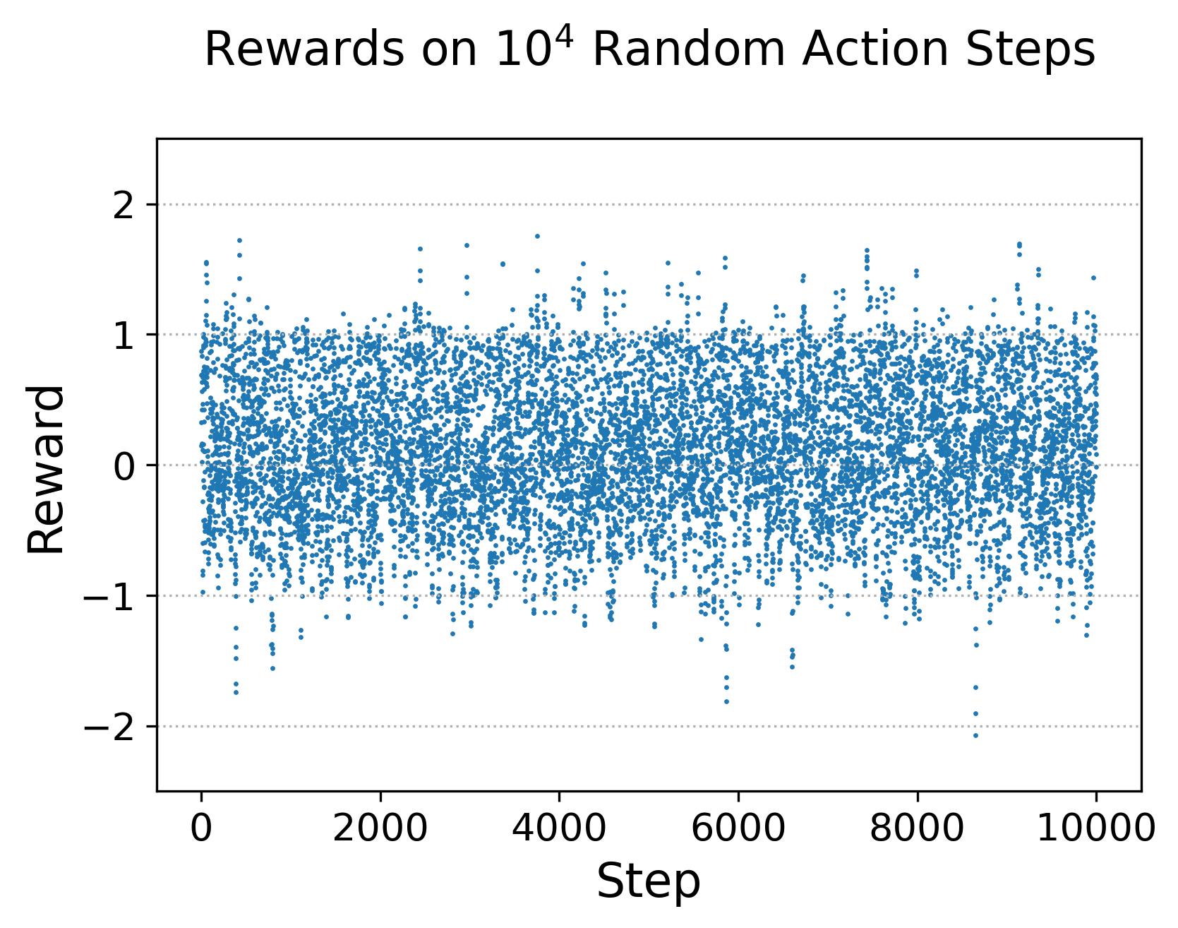
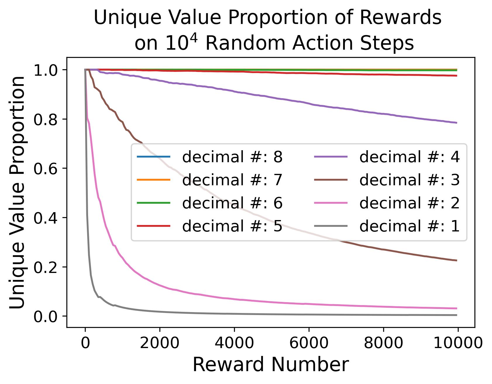
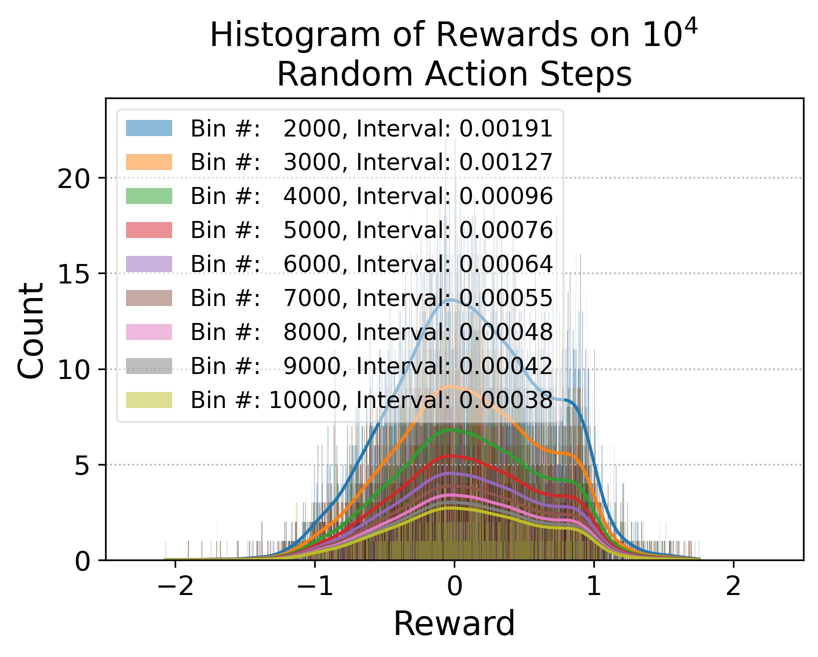
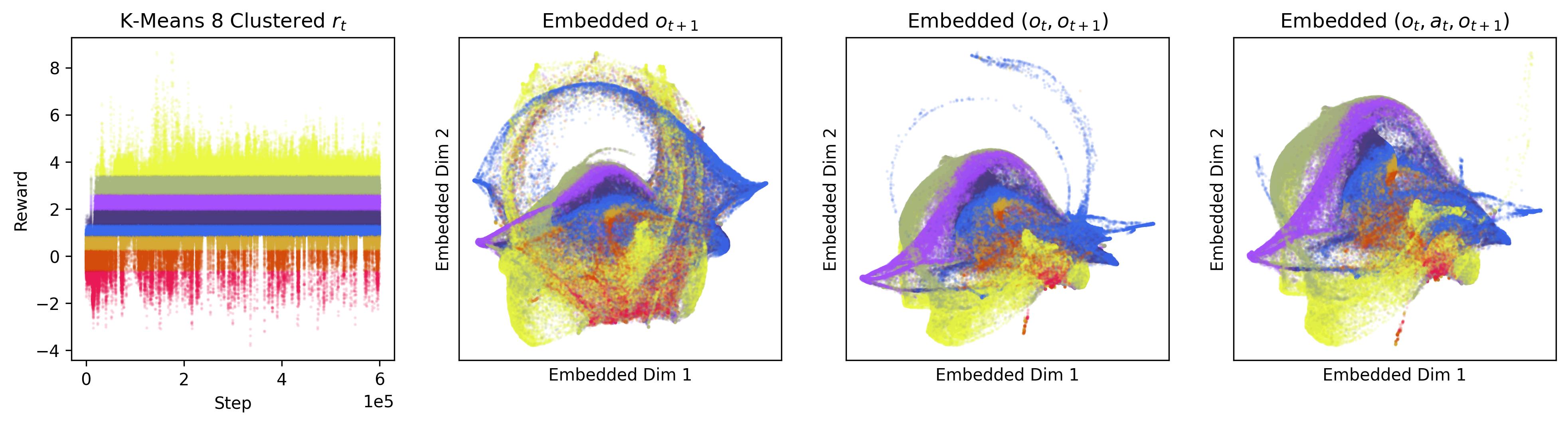
To make the empirical fact, that the dense reward signal can be roughly viewed as a one-dimensional state-transition abstraction of , more intuitive, Fig. 12 shows the rewards collected from random actions, where Fig. 12(a) shows the collected rewards, Fig. 12(b) shows the proportion of the unique reward value rounded to a specific decimal within a chosen reward number, and Fig. 12(c) shows the histograms with various bin number. As shwon in Fig. 12(b), when considering 6 decimal of the reward value, every reward is unique and can be used to different different experiences, even though the difference in the reward may be very small and hard to be detected. To further show the mapping between the reward and state-transition , we firstly cluster the rewards of experiences collected by TD3 on the modified Walker2D (the 1st panel of Fig. 13), then we visualize , , and with the cluster color of the , respectively in the 2nd-4th panel of Fig. 13, by embedding them into 2D using TriMap (Amid and Warmuth, 2019). Note that TriMap is chosen here because its good at maintaining the relative distances of the clusters which is necessary to show that the close rewards correspond to close state-transition. As can be seen from Fig. 13, reward values that are close correspond to , , and are also grouped, where and show tighter groups than indicating reward can be seen as a 1D representation of the state-transition rather than simply the . It is worth to emphasise there is no guarantee TriMap can maintain relative distances of the clusters, even though it has been shown to be better at it than other dimensionality reduction methods, such as PCA and t-SNE.

A.2 Hyperparameters for Algorithms
Table 8 details the hyper-parameters used in this work, where indicates the parameter does not apply to the corresponding algorithm. For the actor and critic neural network structure of LSTM-TD3, the first row corresponds to the structure of the memory component, the second row corresponds to the structure of the current feature extraction, and the third row corresponds to the structure of perception integration after combining the extracted memory and the extracted current feature.
| Hyperparameter | Algorithms | |||||
| PPO | TD3 | MTD3 | SAC | MSAC | LSTM-TD3 | |
| discount factor: | 0.99 | |||||
| -return: | 0.97 | - | ||||
| clip ratio: | 0.2 | - | ||||
| batch size: | - | 100 | ||||
| replay buffer size: | 4000 | |||||
| random start step: | - | |||||
| update after | - | |||||
| target NN update rate | - | |||||
| optimizer | Adam (Kingma and Ba, 2014) | |||||
| actor learning rate | ||||||
| critic learning rate | ||||||
| actor NN structure: | [256, 256] | |||||
| critic NN structure: | [256, 256] | |||||
| actor exploration noise | - | - | - | |||
| target actor noise | - | - | - | |||
| target actor noise clip boundary | - | - | - | |||
| policy update delay | - | 2 | 2 | - | - | 2 |
| entropy regulation coefficient | - | - | - | 0.2 | 0.2 | - |
| history length | - | - | - | - | - | {0, 1, 3, 5} |
| bootstrapping step size | - | - | {2, 3, 4, 5} | - | {2, 3, 4, 5} | - |
A.3 Additional Results
A.3.1 Additional Results on the Generalization of the Unexpected Result on Other Tasks
Fig. 14 shows the learning curves of the investigated algorithms on both MDP- and POMDP-versions of tasks.

A.3.2 Additional Results on Understand the Effect of Multi-step Bootstrapping
Fig. 15 shows the results on the effect of multi-step size on the performance of MTD3 and MSAC on HalfCheetah-v2 and Hopper-v2. Fig. 16 shows results on the effect of multi-step size on the performance of PPO on Ant-v2 and HalfCheetah-v2.
A.3.3 Additional Results on Effect of Accumulated Reward
To validate Hypothesis 3, results on environment using average reward (Eq. 11) and summation reward (Eq. 12) over consecutive rewards are compared with that on environment using the original reward and shown in Fig. 17 and Fig. 18. In Fig. 17, MTD3(5) and MSAC(5) are drawn with solid lines, while TD3 and SAC are drawn with dotted lines. The results on environment with original reward or with accumulated reward are differentiated with different markers. Fig. 18 compares the maximum return over 4 random seeds within 0.8 million steps. In this figure, we use ✓, ✗, and ✓✗ to indicate if the performance of one algorithm on environment using or is better than that of an algorithm on environment using . For example, for where we compare with and , ✓indicates both and outperform , ✗indicates and outperform , and ✓✗ indicates only one of and outperform . Overall, we cannot see there is any consistent performance improvement when using or , even though there are some cases by using or TD3 or SAC gets better performance than using , e.g., outperforms on Ant-v2 POMDP-FLK. Nevertheless, it is quite clear that the performance of TD3 and SAC on environment using either or is not able to achieve comparable performance of the algorithms using multi-step bootstrapping on environment using , e.g., the huge performance gap between and and that of on Walker2d-v2 POMDP-FLK.


A.3.4 Additional Results on Investigating the Effect of the Exploration Strategies
Fig. 19 and 20 show results on other tasks to compare SAC with MSAC(5) and compare TD3 with MTD3(5) in order to investigate the effect of the exploration strategies. Fig. 21 shows the bar-chart of the results of SAC and MSAC(5). Fig. 22 shows the bar-chart of the results of TD3 and MTD3(5). Fig. 23 shows the results on other tasks when investigating the effect of exploration strategy for PPO.
References
- Amid and Warmuth (2019) Ehsan Amid and Manfred K. Warmuth. TriMap: Large-scale Dimensionality Reduction Using Triplets. arXiv preprint arXiv:1910.00204, 2019.
- Arora et al. (2018) Sankalp Arora, Sanjiban Choudhury, and Sebastian Scherer. Hindsight is only 50/50: Unsuitability of mdp based approximate pomdp solvers for multi-resolution information gathering. arXiv preprint arXiv:1804.02573, 2018.
- Bai (2021) Yuqin Bai. An empirical study on bias reduction: Clipped double q vs. multi-step methods. In 2021 International Conference on Computer Information Science and Artificial Intelligence (CISAI), pages 1063–1068. IEEE, 2021.
- Baisero and Amato (2021) Andrea Baisero and Christopher Amato. Unbiased asymmetric reinforcement learning under partial observability. arXiv preprint arXiv:2105.11674, 2021.
- Beynier et al. (2013) Aurelie Beynier, Francois Charpillet, Daniel Szer, and Abdel-Illah Mouaddib. Dec-mdp/pomdp. Markov Decision Processes in Artificial Intelligence, pages 277–318, 2013.
- Cassandra (1998) Anthony R Cassandra. A survey of pomdp applications. In Working notes of AAAI 1998 fall symposium on planning with partially observable Markov decision processes, volume 1724, 1998.
- De Asis et al. (2018) Kristopher De Asis, J Hernandez-Garcia, G Holland, and Richard Sutton. Multi-step reinforcement learning: A unifying algorithm. In Proceedings of the AAAI Conference on Artificial Intelligence, volume 32, 2018.
- Duan et al. (2016) Yan Duan, Xi Chen, Rein Houthooft, John Schulman, and Pieter Abbeel. Benchmarking deep reinforcement learning for continuous control. In International conference on machine learning, pages 1329–1338. PMLR, 2016.
- Dulac-Arnold et al. (2021) Gabriel Dulac-Arnold, Nir Levine, Daniel J Mankowitz, Jerry Li, Cosmin Paduraru, Sven Gowal, and Todd Hester. Challenges of real-world reinforcement learning: definitions, benchmarks and analysis. Machine Learning, 110(9):2419–2468, 2021.
- Foka and Trahanias (2007) Amalia Foka and Panos Trahanias. Real-time hierarchical pomdps for autonomous robot navigation. Robotics and Autonomous Systems, 55(7):561–571, 2007.
- Fujimoto et al. (2018) Scott Fujimoto, Herke Hoof, and David Meger. Addressing function approximation error in actor-critic methods. In International conference on machine learning, pages 1587–1596. PMLR, 2018.
- Gregurić et al. (2020) Martin Gregurić, Miroslav Vujić, Charalampos Alexopoulos, and Mladen Miletić. Application of deep reinforcement learning in traffic signal control: An overview and impact of open traffic data. Applied Sciences, 10(11):4011, 2020.
- Haarnoja et al. (2018) Tuomas Haarnoja, Aurick Zhou, Pieter Abbeel, and Sergey Levine. Soft actor-critic: Off-policy maximum entropy deep reinforcement learning with a stochastic actor. In International conference on machine learning, pages 1861–1870. PMLR, 2018.
- Hausknecht and Stone (2015) Matthew Hausknecht and Peter Stone. Deep recurrent q-learning for partially observable mdps. In 2015 aaai fall symposium series, 2015.
- Henderson et al. (2018) Peter Henderson, Riashat Islam, Philip Bachman, Joelle Pineau, Doina Precup, and David Meger. Deep reinforcement learning that matters. In Proceedings of the AAAI conference on artificial intelligence, volume 32, 2018.
- Hessel et al. (2018) Matteo Hessel, Joseph Modayil, Hado Van Hasselt, Tom Schaul, Georg Ostrovski, Will Dabney, Dan Horgan, Bilal Piot, Mohammad Azar, and David Silver. Rainbow: Combining improvements in deep reinforcement learning. In Thirty-second AAAI conference on artificial intelligence, 2018.
- Hill et al. (2018) Ashley Hill, Antonin Raffin, Maximilian Ernestus, Adam Gleave, Anssi Kanervisto, Rene Traore, Prafulla Dhariwal, Christopher Hesse, Oleg Klimov, Alex Nichol, Matthias Plappert, Alec Radford, John Schulman, Szymon Sidor, and Yuhuai Wu. Stable baselines. https://github.com/hill-a/stable-baselines, 2018.
- Ibarz et al. (2021) Julian Ibarz, Jie Tan, Chelsea Finn, Mrinal Kalakrishnan, Peter Pastor, and Sergey Levine. How to train your robot with deep reinforcement learning: lessons we have learned. The International Journal of Robotics Research, 40(4-5):698–721, 2021.
- Igl et al. (2018) Maximilian Igl, Luisa Zintgraf, Tuan Anh Le, Frank Wood, and Shimon Whiteson. Deep variational reinforcement learning for pomdps. In International Conference on Machine Learning, pages 2117–2126. PMLR, 2018.
- Kingma and Ba (2014) Diederik P Kingma and Jimmy Ba. Adam: A method for stochastic optimization. arXiv preprint arXiv:1412.6980, 2014.
- Krishna and Murty (1999) K Krishna and M Narasimha Murty. Genetic k-means algorithm. IEEE Transactions on Systems, Man, and Cybernetics, Part B (Cybernetics), 29(3):433–439, 1999.
- Lample and Chaplot (2017) Guillaume Lample and Devendra Singh Chaplot. Playing fps games with deep reinforcement learning. In Thirty-First AAAI Conference on Artificial Intelligence, 2017.
- Lillicrap et al. (2015) Timothy P Lillicrap, Jonathan J Hunt, Alexander Pritzel, Nicolas Heess, Tom Erez, Yuval Tassa, David Silver, and Daan Wierstra. Continuous control with deep reinforcement learning. arXiv preprint arXiv:1509.02971, 2015.
- Littman et al. (1995) Michael L Littman, Anthony R Cassandra, and Leslie Pack Kaelbling. Learning policies for partially observable environments: Scaling up. In Machine Learning Proceedings 1995, pages 362–370. Elsevier, 1995.
- Lopez-Martin et al. (2020) Manuel Lopez-Martin, Belen Carro, and Antonio Sanchez-Esguevillas. Application of deep reinforcement learning to intrusion detection for supervised problems. Expert Systems with Applications, 141:112963, 2020.
- Mahmood et al. (2018) A Rupam Mahmood, Dmytro Korenkevych, Gautham Vasan, William Ma, and James Bergstra. Benchmarking reinforcement learning algorithms on real-world robots. In Conference on robot learning, pages 561–591. PMLR, 2018.
- Mandlekar et al. (2021) Ajay Mandlekar, Danfei Xu, Josiah Wong, Soroush Nasiriany, Chen Wang, Rohun Kulkarni, Li Fei-Fei, Silvio Savarese, Yuke Zhu, and Roberto Martín-Martín. What matters in learning from offline human demonstrations for robot manipulation. arXiv preprint arXiv:2108.03298, 2021.
- Meng (2023) Lingheng Meng. Learning to engage: An application of deep reinforcement learning in living architecture systems. 2023.
- Meng et al. (2021a) Lingheng Meng, Rob Gorbet, and Dana Kulić. The effect of multi-step methods on overestimation in deep reinforcement learning. In 2020 25th International Conference on Pattern Recognition (ICPR), pages 347–353. IEEE, 2021a.
- Meng et al. (2021b) Lingheng Meng, Rob Gorbet, and Dana Kulić. Memory-based deep reinforcement learning for pomdps. In 2021 IEEE/RSJ International Conference on Intelligent Robots and Systems (IROS), pages 5619–5626. IEEE, 2021b.
- Mnih et al. (2013) Volodymyr Mnih, Koray Kavukcuoglu, David Silver, Alex Graves, Ioannis Antonoglou, Daan Wierstra, and Martin Riedmiller. Playing atari with deep reinforcement learning. arXiv preprint arXiv:1312.5602, 2013.
- Mnih et al. (2015) Volodymyr Mnih, Koray Kavukcuoglu, David Silver, Andrei A Rusu, Joel Veness, Marc G Bellemare, Alex Graves, Martin Riedmiller, Andreas K Fidjeland, Georg Ostrovski, et al. Human-level control through deep reinforcement learning. nature, 518(7540):529–533, 2015.
- Mnih et al. (2016) Volodymyr Mnih, Adria Puigdomenech Badia, Mehdi Mirza, Alex Graves, Timothy Lillicrap, Tim Harley, David Silver, and Koray Kavukcuoglu. Asynchronous methods for deep reinforcement learning. In International conference on machine learning, pages 1928–1937. PMLR, 2016.
- Morad et al. (2023) Steven Morad, Ryan Kortvelesy, Matteo Bettini, Stephan Liwicki, and Amanda Prorok. Popgym: Benchmarking partially observable reinforcement learning. arXiv preprint arXiv:2303.01859, 2023.
- Ni et al. (2021) Tianwei Ni, Benjamin Eysenbach, and Ruslan Salakhutdinov. Recurrent model-free rl can be a strong baseline for many pomdps. arXiv preprint arXiv:2110.05038, 2021.
- Oliehoek et al. (2016) Frans A Oliehoek, Christopher Amato, et al. A concise introduction to decentralized POMDPs, volume 1. Springer, 2016.
- Ong et al. (2009) Sylvie CW Ong, Shao Wei Png, David Hsu, and Wee Sun Lee. Pomdps for robotic tasks with mixed observability. In Robotics: Science and systems, volume 5, page 4, 2009.
- Pajarinen et al. (2022) Joni Pajarinen, Jens Lundell, and Ville Kyrki. Pomdp planning under object composition uncertainty: Application to robotic manipulation. IEEE Transactions on Robotics, 2022.
- Reda et al. (2020) Daniele Reda, Tianxin Tao, and Michiel van de Panne. Learning to locomote: Understanding how environment design matters for deep reinforcement learning. In Motion, Interaction and Games, pages 1–10. 2020.
- Sandikci (2010) Burhaneddin Sandikci. Reduction of a pomdp to an mdp. Wiley Encyclopedia of Operations Research and Management Science, 2010.
- Satheeshbabu et al. (2020) Sreeshankar Satheeshbabu, Naveen K Uppalapati, Tianshi Fu, and Girish Krishnan. Continuous control of a soft continuum arm using deep reinforcement learning. In 2020 3rd IEEE International Conference on Soft Robotics (RoboSoft), pages 497–503. IEEE, 2020.
- Schulman et al. (2015a) John Schulman, Sergey Levine, Pieter Abbeel, Michael Jordan, and Philipp Moritz. Trust region policy optimization. In International conference on machine learning, pages 1889–1897. PMLR, 2015a.
- Schulman et al. (2015b) John Schulman, Philipp Moritz, Sergey Levine, Michael Jordan, and Pieter Abbeel. High-dimensional continuous control using generalized advantage estimation. arXiv preprint arXiv:1506.02438, 2015b.
- Schulman et al. (2017) John Schulman, Filip Wolski, Prafulla Dhariwal, Alec Radford, and Oleg Klimov. Proximal policy optimization algorithms. arXiv preprint arXiv:1707.06347, 2017.
- Shani et al. (2013) Guy Shani, Joelle Pineau, and Robert Kaplow. A survey of point-based pomdp solvers. Autonomous Agents and Multi-Agent Systems, 27:1–51, 2013.
- Shao et al. (2022) Yang Shao, Quan Kong, Tadayuki Matsumura, Taiki Fuji, Kiyoto Ito, and Hiroyuki Mizuno. Mask atari for deep reinforcement learning as pomdp benchmarks. arXiv preprint arXiv:2203.16777, 2022.
- Singh et al. (2021) Gautam Singh, Skand Peri, Junghyun Kim, Hyunseok Kim, and Sungjin Ahn. Structured world belief for reinforcement learning in pomdp. In International Conference on Machine Learning, pages 9744–9755. PMLR, 2021.
- Subramanian et al. (2022) Jayakumar Subramanian, Amit Sinha, Raihan Seraj, and Aditya Mahajan. Approximate information state for approximate planning and reinforcement learning in partially observed systems. Journal of Machine Learning Research, 23(12):1–83, 2022.
- Sutton and Barto (2018) Richard S Sutton and Andrew G Barto. Reinforcement learning: An introduction. MIT press, 2018.
- Tang (2020) Yunhao Tang. Self-imitation learning via generalized lower bound q-learning. Advances in neural information processing systems, 33:13964–13975, 2020.
- Towers et al. (2023) Mark Towers, Jordan K. Terry, Ariel Kwiatkowski, John U. Balis, Gianluca de Cola, Tristan Deleu, Manuel Goulão, Andreas Kallinteris, Arjun KG, Markus Krimmel, Rodrigo Perez-Vicente, Andrea Pierré, Sander Schulhoff, Jun Jet Tai, Andrew Tan Jin Shen, and Omar G. Younis. Gymnasium, March 2023. URL https://zenodo.org/record/8127025.
- Tunyasuvunakool et al. (2020) Saran Tunyasuvunakool, Alistair Muldal, Yotam Doron, Siqi Liu, Steven Bohez, Josh Merel, Tom Erez, Timothy Lillicrap, Nicolas Heess, and Yuval Tassa. dm_control: Software and tasks for continuous control. Software Impacts, 6:100022, 2020.
- Van der Maaten and Hinton (2008) Laurens Van der Maaten and Geoffrey Hinton. Visualizing data using t-sne. Journal of machine learning research, 9(11), 2008.
- Van Hasselt et al. (2016) Hado Van Hasselt, Arthur Guez, and David Silver. Deep reinforcement learning with double q-learning. In Proceedings of the AAAI conference on artificial intelligence, volume 30, 2016.
- van Seijen (2016) Harm van Seijen. Effective multi-step temporal-difference learning for non-linear function approximation. arXiv preprint arXiv:1608.05151, 2016.
- Wang et al. (2016a) Ziyu Wang, Victor Bapst, Nicolas Heess, Volodymyr Mnih, Remi Munos, Koray Kavukcuoglu, and Nando De Freitas. Sample efficient actor-critic with experience replay. arXiv preprint arXiv:1611.01224, 2016a.
- Wang et al. (2016b) Ziyu Wang, Tom Schaul, Matteo Hessel, Hado Hasselt, Marc Lanctot, and Nando Freitas. Dueling network architectures for deep reinforcement learning. In International conference on machine learning, pages 1995–2003. PMLR, 2016b.
- Weng et al. (2022) Jiayi Weng, Huayu Chen, Dong Yan, Kaichao You, Alexis Duburcq, Minghao Zhang, Yi Su, Hang Su, and Jun Zhu. Tianshou: A highly modularized deep reinforcement learning library. Journal of Machine Learning Research, 23(267):1–6, 2022. URL http://jmlr.org/papers/v23/21-1127.html.
- Yoon et al. (2008) Sung Wook Yoon, Alan Fern, Robert Givan, and Subbarao Kambhampati. Probabilistic planning via determinization in hindsight. In AAAI, pages 1010–1016, 2008.
- Zhang et al. (2019) Zidong Zhang, Dongxia Zhang, and Robert C Qiu. Deep reinforcement learning for power system applications: An overview. CSEE Journal of Power and Energy Systems, 6(1):213–225, 2019.