Experimental Results on Potential Markov Partitions for Wang Shifts
Abstract.
In this article we discuss potential Markov partitions for three different Wang tile protosets. The first partition is for the order-24 aperiodic Wang tile protoset that was recently shown in the Ph.D. thesis of H. Jang to encode all tilings by the Penrose rhombs. The second is a partition for an order-16 aperiodic Wang protoset that encodes all tilings by the Ammann A2 aperiodic protoset. The third partition is for an order-11 Wang tile protoset identified by Jeandel and Rao as a candidate order-11 aperiodic Wang tile protoset. The emphasis is on some experimental methodology to generate potential Markov partitions that encode tilings. We also apply some of the theory developed by Labbé in analyzing such an experimentally discovered partition.
Key words and phrases:
Aperiodic tiling and Wang shift and SFT and Multidimensional SFT and Nonexpansive directions2020 Mathematics Subject Classification:
Primary 37B51; Secondary 37B10, 52C231. Introduction
1.1. Tilings and Aperiodic Protosets
A tiling of the Euclidean plane is a collection of distinct sets called tiles (which are typically topological disks) such that and for all , . A protoset for a tiling is a collection of tiles such that each tile of is congruent to a tile in , in which case we say that admits the tiling . The symmetry group of a tiling is the set of rigid planar transformations such that for all . If contains two nonparallel translations, we say that is periodic; otherwise, we say is nonperiodic. If admits at least one tiling of the plane and every such tiling is nonperiodic, we say that is an aperiodic protoset.
Aperiodic protosets are somewhat rare, and indeed, until the 1960s, no aperiodic protosets were known to exist. H. Wang famously conjectured that aperiodic protosets cannot exist [Wan61]; that is, Wang conjectured that any protoset that admits a tiling of the plane must admit at least one periodic tiling. Wang’s conjecture was refuted in 1964 by his doctoral student, R. Berger, in his PhD thesis [Ber65, Ber66] where an aperiodic protoset consisting of over 20,000 edge-marked squares called Wang tiles was described. Wang tiles are a bit of a special case in the theory of tilings in that only translations are allowed in forming tilings from Wang tile protosets; if rotations and reflections are also allowed, then any single Wang tile admits periodic tilings of the plane, and so without this restriction the problem is trivial. Since Berger’s original discovery, several lower-order aperiodic Wang tile protosets have been discovered, culminating in 2015 with the discovery by E. Jeandel and M. Rao [JR21] of an order-11 aperiodic Wang tile protoset. In this same work the authors proved that 11 is the minimum possible order for an aperiodic Wang tile protoset. The aperiodic Jeandel-Rao protoset is seen in Figures 1, and here we are using the same labeling for the Jeandel-Rao protoset as given by Labbé in [Lab21].

Aperiodic protosets of tiles other than Wang tiles are also known. In 1971, R. Robinson developed a way to encode the idea of Berger’s original aperiodic protoset into an order-6 aperiodic protoset consisting of shapes with notched edges and modified corners (Figure 2(a)). In 1974, R. Penrose discovered an order-6 aperiodic protoset that he was later able to modify to produce an order-2 aperiodic protoset. There are a few varieties of the order-2 aperiodic Penrose protoset, one of which, called P3 or the Penrose rhombs, is depicted in Figure 2(b); this protoset will be discussed further this article. More recently, in 2023 two singleton aperiodic protosets was discovered ([Smi+23a, Smi+23]) - these “aperiodic monotiles” are called the hat (Figure 2(c)) and spectre (Figure 2(d)); we note that no edge-matching rules are needed to enforce nonperiodicity with the hat and spectre, unlike the Penrose rhombs, for example.


1.2. Labbé’s Markov Partition for the Jeandel-Rao Protoset
Let be the aperiodic Jeandel-Rao Wang tile protoset (Figure 1). The set of all tilings admitted by is called the Jeandel-Rao Wang shift and is denoted . In [Lab21], S. Labbé presented a special partition (Figure 3) of the two-dimensional torus , along with a action on , that together give rise tilings in . Specifically, let be the golden mean and let be the lattice in generated by and . Then the partitioned torus is and the action on is defined by .
Here we describe how the partition of and the action encode tilings by . Let and consider the orbit . Then corresponds to a tiling in in the following way:
This idea is depicted in Figure 3. There are several technical details that Labbé proved so that the correspondence between orbits of points in the partitioned torus correspond to tilings in an unambiguous way, but this is the gist of it. It is interesting - even somewhat amazing - that most tilings admitted by are encoded by and !
In this article, we present some partitions, discovered experimentally, that are analogous to the Markov partition for the Jeandel-Rao protoset, but for other Wang tile protosets. Further, we discuss how to identify other potential Markov partitions for Wang shifts in which tilings exhibit “golden rotational” behavior similar to with . We will also discuss theoretical framework described by Labbé in [Lab21] and apply it to one of these new partitions in an effort to describe the full space of tilings arising from the partition.
2. Labbé’s Construction
While we are focussed on an experimental approach in this article, it will be necessary to describe some of the technical details of Labbé’s construction, which are described in the language of dynamical systems. For now, we want to keep this discussion as non-technical as possible to focus on the big picture ideas, and we will provide more technical apsects in Appendix A. In that spirit, let us start by describing Wang tilings in the language of dynamical systems. This begins by defining Wang tilings in a very symbolic way.
2.1. Spaces of Wang Tilings as Dynamical Systems
Geometrically, a Wang tile is a square with labeled (or colored) sides that serve as edge matching rules; two Wang tiles may meet along an edge if corresponding labels match. In forming a Wang tiling from copies of tiles in a protoset of Wang tiles, we allow only translates of the prototiles to be used, and we require that the tiles to meet edge-to-edge, respecting the matching rules. The edge-to-edge matching rules and restriction to translations can always be enforced geometrically, as in Figure 1. Wang tilings can be aligned with the integer lattice so that each tile has its lower left-hand corner in , and thus we may view a Wang tiling as a decoration of such that each point of is “colored” with a single tile.
More formally, a Wang tile can be represented as a tuple of four colors where and are finite sets (the vertical and horizontal colors, respectively). For any Wang tile , let , , , and be the colors of the right, top, left, and right sides of , respectively. Let be a protoset of Wang tiles. In forming a tiling with the protoset , we will think of the prototiles of as symbols used to label the integer lattice . This motivates us to define
to be the configuration space of , and each element is called a configuration. We will use the notation to indicate the value of at so that if we understand that tile is located at position (i.e,, oriented so that its corners lie in and the lower left-hand corner is at ). It is possible that a configuration in does not represent a valid tiling; so far, this construction does not account for the matching rules of the tiles. To account for the matching rules, we define a configuration to be valid if for every , we have and . The Wang shift of is the set of all valid configurations in . Thus, captures in a symbolic way the set of all valid Wang tilings admitted by the Wang tile protoset .
A topological dynamical system consists of a topological space and a group that acts on via a continuous function , and is denoted by a triple . For fixed , let be defined by . The orbit of a point under the action of on is the set , and when the group is understood by context, we will shorten this notation to just . We say acts freely on if for all , if and only if where is the group identity element.
Let be defined by . We call the shift action on ; the terminology “shift action” is accurately descriptive here since, for each and , is a translation of by . By placing the appropriate metric on , it is not too hard to see that is a topological space so that satisfies the definition of being a topological dynamical system. Moreover, is a special kind of topological dynamical system called a shift of finite type (see Appendix A).
If acts freely on , we say that is an aperiodic shift, and we say that a Wang protoset is an aperiodic protoset if the corresponding Wang shift is nonempty and aperiodic. Notice that this definition for aperiodic protoset agrees with with more general definition given in Section 1.1 if we restrict the allowable symmetries to translations only.
2.2. Labbé’s Partition-Based Dynamical System of Tilings
Here we will provide the broad strokes of Labbé’s [Lab21] general approach and construction of the dynamical system that is based on a partition of a compact topological space and a action on . The space is the set of tilings encoded by the partition and the action , as exemplified by Figure 3. We will relegate much of the more technical details to Appendix A. The main point is that methodologies are described in [Lab21] that can be used to prove when and produce a space that is reasonable subspace (or subshift) of the space of all valid tilings admitted by .
First, let be a compact metric space and let . A collection of disjoint open sets with is called a topological partition of , and the sets are called the atoms of the partition. Let is a topological partition of , and let be a protoset of Wang tiles having the same indexing set as . Let be a action on . Then is a topological dynamical system, and with so partitioned by , the hope is that the orbit of a point will “spell out” a tiling in . More precisely, for each , we can consider the orbit , and for each , define the configuration in by
The configuration may not be not well defined because for some , the point may lie on the boundary of more than one atom of . However, Labbé [Lab21] was able prove that this ambiguity can be removed in the following way: By specifying a direction that is not parallel to any of the sides of the atoms of the partition, then if a point falls on the boundary of an atom, the choice of tile associated with that point is the one in the direction of from . In this way, each point can be associated uniquely with a configuration , thereby defining a mapping (“” for “symbolic representation”). With this map properly defined, we obtain the space of interest, , as the topological closure of the image of :
Labbé [Lab21] shows that the choice of doesn’t actually matter after taking the topological closure, so the space is not dependent on . Figure 3 is worth a thousand words in understanding the essential function of . In that figure, we see how the points of the orbit of a point in the torus forms a configuration of Wang tiles.
We pause here to point out that the space is fully defined in more technical terms in [Lab21] that facilitate the use of the tools of dynamical systems to prove that if the partition and the action satisfy reasonable technical properties, the partitioned system gives rise to along with morphims going both directions. With such formalisms in place, important properties of the space can be determined. For example, we are interested in knowing when is shift of finite type, which is an important property that a Wang shift has. Another important proptery is minimality of the subshift, which can be deduced from properties of the partition and action.
At this point, it may be believable that is a reasonable subset of , so configurations of can be seen as potential valid configuations (i.e. tilings), but it should not be clear at all how the partition “knows” what the edge matching rules are and how orbits of points correspond to valid tilings that respect the matching rules of the prototiles of . This is where some magic occurs in the Labbé construction. The magic is that the partition needs to be a refinement of four other partitions , , , and called side partitions that encode the matching rules of prototiles in . With these side partitions suitably defined, the main partition is defined as . With so defined, and checking that has certain necessary dynamical properties, it is argued in [Lab21] that . That is, the configurations generated from orbits of points in the partitioned set are valid tilings! We use the word “magic” here to describe the process of finding because there is no simple formula for finding such a partition. For a given Wang protoset , the partition may be found through some educated guesswork and the help of computers. In the next section, we will describe an experimental approach to finding partitions.
3. Finding Partitions Experimentally
Let us return to the Jeandel-Rao aperiodic protoset and Labbé’s corresponding Markov partition from Figure 3. Recall that in this construction we have where is generated by and . Given a tiling , we will attempt to recover the partition . Suppose that is “generated” from the orbit of a point , using the partition and the action . Without loss of generality, we may (by shifting the orientation of the partition ) suppose that . For each , let . By definition of , we have
| (1) |
Recall the manner in which the partition encodes the tiling: If , then a copy of prototile is located at position .
Now, working backward, suppose we have a tiling generated by the orbit , but after generating , let us pretend that we have lost all knowledge of the partition. If we colored the points according to the label of the tile located at position , then the colored set of points
| (2) |
would appear as a dense set of points in the rectangle , and the coloring of the points would reveal the partition .
Our goal here is to demonstrate that a partition associated with a Wang shift can be revealed by looking at specific tilings in the Wang shift without prior knowledge of the partition. By Equation 1, for each , there exists some such that
| (3) |
where
is the matrix whose columns are the generating vectors of . From Equation 3, we obtain . Because , it follows that
| (4) |
Let
and assign to each the color if a copy of prototile is located at position . From Equation 4, we see that the set is just a linearly transformed copy of the original dense set of colored points , and recall that reveals the partition . Therefore, we see that , being a linear transformation of , reveals a partition that is essentially equivalent to the original .
If the only knowledge we have at the beginning of this process is that of a tiling or a large finite portion of a tiling (perhaps generated by a computer algorithm), then we may not be immediately privy to the matrix (i.e., the generating vectors of the lattice that forms the torus) whose inverse we would use to pull back the tiling to obtain a partition, but the tiling itself may give clues about this matrix. In fact, Labbé discovered the partition in exactly this way - by noticing some Sturmian-like patterns in the rows of a large patch of a Jeandel-Rao tiling that suggested the correct vectors by which to “mod-out.” Finding the matrix is the key to this strategy.
To see how this experimental approach reveals the partition (once you have guessed the correct generating vectors for the lattice), let us first use Labbé’s Sagemath package ([Lab23]) to produce a tiling of a given size. Here we produce a 100x100 patch of a Jeandel-Rao Wang tiling:
Next, from the tiling so produced, we can pull back the points of the tiling to the unit square and color each using the label of the tile from which it came.
Here is the picture so produced:

Comparing Figures 3 and 4, we see that the dot pattern does indeed capture the atoms of the original partition. It should be noted here that the tiling used to generate the colored dot pattern was not produced using the partition ; instead, it was produced using the Glucose solver, which implements a brute force method to finding a tiling. This suggests that the partition is fundamental to the space , which is the main thrust of what Labbé proved in [Lab21].
4. The Penrose and Ammann Wang Shifts
In [GS87, Section 11.1], the authors discuss methods for converting low-order aperiodic protosets into low-order aperoidic Wang tile protosets, including the order-2 Penrose aperiodic protosets P2 and P3 and the order-2 Ammann aperiodic protoset A2. In particular, there we find an outline of how to convert Penrose tile protosets to two different aperiodic Wang tile protosets - one of order 24 (from P3) and one of order 16 (from P2). We also find that the Ammann A2 protosets can be converted to an order 16 Wang tile protoset, which, interestingly, is the exact same order-16 Wang tile protoset obtained from the Penrose P3 protoset, suggesting that P2 and A2 are really the same on some fundamental level. More recently, in H. Jang’s recent Ph.D. thesis [Jan21, Lemma 6.2.2, p. 75], it was shown that any tiling by Penrose rhombs P3 is equivalent to a Wang tiling from the set of 24 Wang tiles mentioned above.
4.1. The Order-24 Penrose Wang Tile Protoset
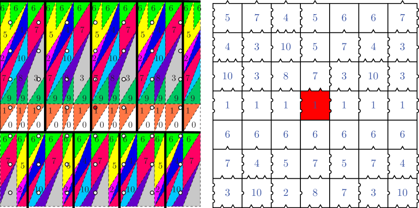
Following the method suggested in [GS87, Section 11.1], a tiling by the Penrose rhombs (P3) can be coverted to a tiling by Wang tiles using the patches of tiles shown in Figure 5. This protoset of 24 Wang tiles, as was proven in [Jan21], produces tilings in exact correspondence with the tilings produced by the P3 protoset.


Let the protoseet of Figure 6 be denoted by . We may use the computer to produce a large patch of tiling, and then using a matrix
we can produce a dot pattern that reveals a partition for .

From this dot pattern, we can guess at the exact slopes of the lines and produce an exact partition of the torus , viewed as a quotient of the unit square. We have created such a partition in Figure 8. To simplify things, at right Figure 8 we have scaled the partition by a factor of to obtain a partition , and we may consider the torus where with action defined on by . From these ingredients, we can now consider the space and testable hypotheses concerning that space that lends itself to the techniques developed by Labbé in [Lab21], such as:
-
•
Are configurations in always valid tilings in ? I.e., Is ?
-
•
Is a shift of finite type?
-
•
Is minimal in ?
-
•
Is it true that , so that the partition produces all possible Penrose tilings?
-
•
Will exhibit nonexpansive directions, as corresponding space did for the Jeandel-Rao shift?

We will pursue questions such as these in Appendix B, but for now, we will continue with this experimental approach to finding a few other potential interesting partitions for Wang tile protosets.
4.2. The Order-16 Ammann A2 Wang Tile Protoset
The Ammann A2 order-2 aperiodic protoset is shown in Figure 9. Notice at bottom in Figure 9 that the tiles are adorned with red and blue lines called Ammann bars. The matching rule is that when two copies of tiles from A2 meet, Ammann bars of the same color must continue in a straight line. In Figure 10, we see how the matching rules are enforced in a small patch of tiling for the A2 protoset.


The key to converting the A2 protoset to a Wang tile protoset of order 16 is to consider all of the possible rhombi formed from the red lines, with the blue lines serving as the matching rules for the red rhombi, as explained in In [GS87, Section 11.1]. The protoset so produced, , is shown in Figure 11.

Again, as we did with the , we can use the computer to produce a large patch of tiling, and with the appropriate choice of matrix, we can pull the tiling back onto a torus and see a dot pattern that indicates that a partition underlies the protoset. Indeed, using
we obtain the nice dot pattern shown in Figure 12. Interestingly, we see not only that , but also that the dot patterns for and align - the pattern for P3 seems to be a refinement of the one for A2 (Figure 13). This is not coincidental. In [GS87, Section 11.1] it is pointed out that can be derived from the Penrose darts and kites (P2) protoset using the idea of Ammann bars.


From the dot pattern obtained for , we can determine the exact equations of the lines to get a partition , as shown in Figure 14. We have scaled the partitioned torus for by a factor of (as we did for ). Define the torus identifying opposites sides of this square and define the action on by . We may now consider the space and consider questions like those outlined in Subsection 4.1.

4.3. Testing and
Before considering more technical theoretical questions about and , we will test, experimentally, if the configurations in these spaces seem to be valid tilings. In doing so, we will consider orbits of points on the torus that intersect the boundary and points whose orbits do not.
Let where has partition and let . We then consider the orbit . We wish to see if the tiling (or at least a finite portion we can generate) spelled out by seems to be valid. This process could be automated, but we will do it “by hand”, drawing the orbit in Figure 15 and the corresponding partial configuration in Figure 16. Notice that the partial tiling so generated is valid. Also note that we could easily convert the Wang tiling of Figure 16 into a tiling by the Penrose rhombs (P3) simply by substituting the patches described in Figure 5 for the corresponding Wang tiles. Similarly, in Figure 17 we see part of the orbit of the point in the torus partitioned by the corresponding partial tiling by the order-16 Ammann Wang tiles () in 18, which again appears to be valid.
It is not hard to check that the orbit of any point , under either action or , will be dense in . Thus, one immediate consequence of and being subspaces of and (respectively) is that the areas of atoms in and correspond to the proportion of tiles of specific kinds in tilings. For example, the area of the atom labeled in (Figure 14) is , which comprises of the area of the torus . This means that in any tiling in , about 14.59% of the tiles will be copies of the prototile .


4.4. Orbits that intersect the boundary of
Let be the union of the boundary lines of the atoms in . In this subsection we consider an example where the orbit of a point in intersects , and we note that the details are similar in . We will illustrate by example how the ambiguity that arises in assigning tiles to points in the orbit on is resolved and we will see a certain interesting phenomenon in the dynamics of .
Let and let . Notice that lies at the intersection of lines of all 4 slopes of boundary lines in since this torus is formed as a quotient by identifying opposite sides. Also notice that lies on a boundary segment of slope connecting and . Consider the orbit . Using the computer, inside of a finite window of size , we can check which points satisfy , and a plot of these points is shown in Figure 19(a). Similarly, inside the same size window, we plot the points satisfying in Figure 19(b). Interestingly, we find that the points where the orbit falls on the boundary forms straight strips of points, sometimes a single strip (when the orbit touches lines in the boundary of just one slope) or four separate strips (when the orbit touches lines in the boundary of different slopes). The directions of the strips are called the nonexpansive directions of . In [LMM22], the authors provide methodology for determining the exact directions of such nonexpansive directions, and we leave that topic for the reader to explore further. We only mention here that these nonexpansive directions correspond to what are commonly called Conway worms in Penrose tilings [Gar97]; nonexpansive directions provides a very nice and more general explanation for such behavior in some tilings.
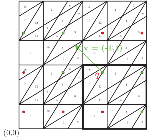
In either situation, the ambiguity in the corresponding tiling can be resolved by choosing a direction to determine what tile to place at the points such that lies on . For example, if we again consider the orbit where is as in Figure 19(b), let us specify a direction vector . Notice that no line segment in is parallel to . Now, at each point of where intersects , place vector with its initial point at . Because is not parallel to any of the segments comprising , then is pointing from into one of the atoms . Thus, we can place a copy of prototile at . The other choice is use to determine the choice of tile at each such point , which points toward the region on the opposite side of the boundary segment as does . This is illustrated in Figures 20 and 21.


5. Candidate Jeandel-Rao Aperiodic Protosets
In [JR21], the authors provide 33 candidate order-11 aperiodic protosets; the computer algorithm that they used to find the aperiodic set could not rule out these 33 candidate sets as ones that admit periodic tilings, so it is likely that they are aperiodic protosets. In any event, as a matter of investigation, we will consider one of these candidate sets as an example. This set, depicted in Figure 22, we will call .

We find that the lattice associated with the original Jeandel-Rao aperiodic protoset does not resolve a coherent dot pattern. However, a variation of does: Define to be the lattice in generated by the vectors and . We see that does succeed in resolving a clear dot pattern, shown in Figure 23. Noticing that this dot pattern is very similar to the partition , it is not hard to arrive at a precise partition for , which is shown in Figure 24. Finally, it appears, at least experimentally, that using the action defined on the torus that is endowed with the partition , produces valid tilings (see figure 25). Perhaps an analysis of the dyanamical systems properties of can be leveraged to argue that the full Wang shift is aperiodic or has other interesting properties.


z
6. Identifying the Signature of the Underlying Lattice
Here we discuss some methodology for determining the lattices for Wang shifts such as , , and . Let be some protoset of Wang tiles, and suppose that there is a hidden encoding of tilings in via a action on a partitioned torus, as with the Wang shifts discussed above. Then there is a lattice generated by vectors and giving rise to a torus , along with a action on defined by , and there is a topological partition of used to encode the orbits of points in under as tilings.
When we look at a tiling in , we may notice the repeating patterns within the tiling that suggest “golden” rotations are responsible for the patterns. Such rotations have some signature behavior, such as having “near periods” of length approximately equal to Fibonnaci numbers and encoding infinite patterns that are in correspondence with the Fibonacci word. An example of such a golden rotation is a 1-dimensional action (rotation) of the unit interval defined by . We partition into two subintervals and . We can use the action and the partition to encode points in as bi-infinite sequences as follows: For each and , if , we place 0 at the -th decimal place of a binary decimal expansion, and if , we place 1 at the -th decimal place. For example, if we encode according to this scheme, we get the bi-infinite binary decimal expansion
which is the well-known Fibonacci word. The presense of repeating patterns in a tiling along a line that follow the pattern of a Fibonacci word suggests that the toral rotation in the direction of that line is something akin to .
Another signature is the spacing of repeating structures. Going back to , consider the orbit of some point . It is not hard to check that is dense in . Thus, there are many values of such that . For what values of is ? It turns out that when is a Fibonacci number, we see that . This is a result of a property of the Fibonacci sequence which has the well-known property that as . From this limit, we see that a Fibonacci number (which is integer valued) is approximately a multiple of . Thus, we see that whenever is Fibonacci. The upshot here is that we expect to see repeating patterns within the encoding of with spacing between these patterns being Fibonacci numbers.
Slightly generalizing the rotation , we may consider rotations of the interval () defined by . Whatever partition we place on , in the encoding of under , we expect to see repeating patterns with spacing between these patterns being Fibonacci numbers because when is approximately a multiple of , which again happens when is a multiple of , which happens when is a Fibonacci number. Thus, seeing a repeating pattern with gaps between being the size of Fibonacci numbers is suggestive of a rotation of the form .
Now let us consider 2-dimensional toral rotations of a certain form: Suppose is defined on a torus by where , , and and () are the generating vectors of the lattice . If is horizontal, then when is restricted to those values of where is fixed, will behave like a golden rotation in the horizontal direction. Thus, to pick up the signature of horizontal golden rotation in a tiling, we look for repeating horizontal patterns in the tiling that have spacing between these patterns being Fibonacci numbers. A similar thing could happen in the vertical direction or any slant direction; in a slant direction, we would look for a repeating pattern with spacing that is a Fibonacci number multiple of a vector parallel to that direction.
While spotting the tell-tale behavior of a golden rotation in a direction inside a tiling is not too difficult to do, finding this direction is of the form and finding the specific values of and are two different questions. We have not yet discovered a way to pinpoint these values from properties of the tiling, but it is not too hard to have the computer test values of and over a range of integers, say where each variable ranges over integers between -3 and 3, and see if any of those values produce dot patters indicating clear partitions. And this is exactly what one can do to find dot patterns for the partitions , , , and .
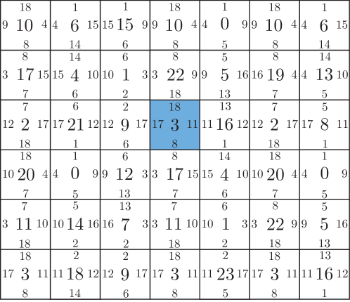
As an example, consider the computer generated partial tiling admitted by (the Wang tile version of the Ammann A2 protoset) shown in Figure 26. Tile 15 has been colored to make it stand out in contrast to the other tiles of the tiling. One notices the signatures of golden rotations within this tiling in both the horizontal and vertical directions - See Figure 26. This is suggestive of golden toral rotations in vertical and horizontal directions of the form and , and luckily, the simplest vectors and produce a nicely resolved dot pattern from which we determined the parittion for .

Other tilings exhibiting golden rotations do not give up their secret lattices quite as easily. For example, in Figure 27, we give a portion of a tiling admitted by the Jeandel-Rao candidate aperiodic protoset . Using the computer to find clearly resolved dot patterns turned up a few essentially equivalent possibilities, one of which is depicted in Figure 23. The golden rotational behavior (Fibonacci spacing) corresponding to the two vectors generating that dot pattern is illustrated in Figure 27.

d
We conclude this section by giving a snippet of code that show how we found the lattice vectors for that produced a clearly resolved dot pattern, revealing the underlying partition.
Acknowledgements
The authors would like to thank Sébastien Labbé for his helpful suggestions.
Appendix A Dynamical Systems and Wang Tilings
Here we will dive a little deeper into the Labbé’s theory, given more definitions and citing several theorems, then applying it to prove some facts about . First, we provide some additional details and definitions, following the ideas laid out in [Lab21].
Recall from Subsection 2.1 that a topological dynamical system is a triple where is a topological space, is a topological group, and is a continuous function which defines a left action of on . For , we will use to indicate the topological closure of in . We also define another kind of closure - the -closure - by , and we will say that is -invariant if . We say the system is minimal if contains no proper, nonempty, (topologically) closed, -invariant subsets.
Recall from Subsection 2.1 that the configuration space, , where is a Wang tile protoset, is thought of as the space of all possible tilings (valid and nonvalid) of the plane by . The configuration space is a topological space when endowed with the compact product topology, and moreover, this topology is generated by the metric on defined by . In the formula for this metric, is a value of closest to the origin where and do not agree, so is close to 0 when and agree on a large patch centered at the origin, and is close to 1 when and disagree near the origin. , where is the shift action, is a topological dynamical system, and in this particular setting, if is -invariant, we say is shift-invariant. For a space of Wang tilings (say, a space of Wang tilings admitted by a protoset, or a space of tilings having some defining property), shift-invariance is clearly a desirable property, for if where , that just means is a translation of , so and are really the same tilings, and thus, we would want to contain both. If is topologically closed and shift invariant in , then we call a subshift of . Notice that is a topological dynamical system when is a subshift of .
A.1. Shifts of Finite Type
Of particular importance in the context of tilings are shifts of finite type. A subshift of Wang tilings being a shift of finite type essentially means, informally, that the tilings in are completely determined a set of forbidden arrangements of tiles, such as when two tiles cannot be placed adjacent to one another due to a mismatch in the edge matching rules. Formally, to define shift of finite type, for any finite subset , we define }, and we call any element a pattern. Next, we define the projection map which restricts any configuration to (i.e. ). We say is a shift of finte type (SFT) if there exists a finite set of patterns called forbidden patterns such that
It is clear that the full Wang shift of a protoset of Wang tiles is an SFT - the set of finite set forbidden patterns is formed simply as a set of representative invalid horizontal and vertical pairings of tiles from the protoset. However, for a subshift of , such as formed from a partition, it may take some work to argue that is an SFT, for it is possible that has forbidden patterns in addition to the invalid horizontal and vertical pairings of prototiles.
A.2. Symbolic Representations and Markov Partitions
Here will will give precise definition to the term Markov partition. Suppose that is a topological dynamical system where is a compact topological space. Recall that a topological partition of is a collection of disjoint open sets such that . Let . For any finite set , let . A pattern is allowed for if
We denote the set of all allowed patterns for and by . Labbé points out in [Lab21] that is the language of a subshift of and leads to the following definition.
Definition A.1.
Let
We call the symbolic dynamical system corresponding to .
For and , define
We see that is compact and for each , and consequently, .
The hope is that configurations are generated uniquely as orbits of points in , and the above intersection being a single point guarantees this:
Definition A.2.
A topological partition of gives a symbolic representation of if for every , the intersection consists of exactly one point . The configuration is called a symbolic representation of .
Labbé provides the following alternative criterion for determining when a partition gives a symbolic representation.
Lemma A.3 ([Lab21]).
Let be a minimal dynamical system and be a topological partition of . If there exists an atom which is invariant only under the trivial translation in , then gives a symbolic representation of .
The following definition is taken from [Lab21].
Definition A.4.
A topological partition of is a Markov partition for if
-
•
gives a symbolic representation of and
-
•
is a shift of finite type (SFT).
A.3. Conjugacy and Factor Maps
With and encoding a space of configurations , it is natural to consider morphisms from to and vice versa. Let and be topological dynamical systems having the same group G. A homomorphism of dynamical systems is a continuous map such that for all . If is a homomorphism, we call an embedding if it is one-to-one; we call a factor map if it is onto, in which case we call a factor of and an extension of ; and we call a topological conjugacy if it is bijective with continuous inverse, in which case we say and are topologically conjugate.
A.4. From Symbolic Representations to Wang Shifts
Here we borrow more theory from [Lab21]. The idea that we want to make precise is that when gives a symbolic representation of , there is a protoset such that ; if happens to be the protoset of interest (i.e., the protoset you used to generate the dot pattern which in turn you used to form ), then we have necessary result that orbits of points under the action of in and the partition encode valid tilings.
Suppose is a topological partition of the 2-dimensional torus , and suppose that gives a symbolic representation of . The boundary of is the set
and
is the set of points in whose orbits intersect . It can be seen that is dense in . We will assume that consists of straight line segments.
We get the following from [Lab21]:
Proposition A.5.
[Lab21, Prop. 5.1] Let give a symbolic representation of the dynamical system such that is a -rotation on . Let be defined such that is the unique point in the intersection . The map is a factor map from to such that for every . The map is one-to-one on .
Following Section 4 of [Lab21], for each , we define a map by
(“Cfg” for “configuration”). gives rise to a map defined by
(“SR” for “symbolic representation”). Next, we wish to extend SR to a map on all , including . This is accomplished by choosing a direction that is not parallel to any of the lines comprising , and then defining by
The idea here is that if , there is ambiguity as to which atom’s label is assigned to by Cfg; the direction settles that ambiguity by assigning to the label of the atom on the side of where lies.
The following lemma from [Lab21] characterizes in terms of map SR.
Lemma A.6.
For each dirction not parallel to a line segment in , we have
where the overline indicates topological closure in the compact product topology on .
We summarize further pertinent results from [Lab21] here:
-
(1)
is 1-1, and so
-
(2)
the inverse map can be extended to the factor map such that for each configuration , (so is as defined in Proposition A.5).
-
(3)
is 1-1 on .
-
(4)
The factor map commutes the shift actions on and on ; that is, .
Using the factor map and these properties of , Labbé proved the following important fact [Lab21]:
Lemma A.7.
Suppose gives a symbolic representation of . Then
-
(1)
if is minimal, then is minimal, and
-
(2)
if is a free -action on , then is aperiodic.
The last results we quote from [Lab21] pertain to understanding how a topological partition gives rise to Wang tile protoset such that . To that end, suppose that is a dynamical system, let (the right side partition) and (the bottom side partition) be two finite topological partitions of , and then let (the left side partition) and (the top side partition); the labels of the atoms of and (i.e. the set ) are the colors of the right and left sides of tiles in a soon-to-be-defined Wang tile protoset, and the labels of the atoms of and (i.e. the set ) are the colors of the top and bottom sides in that same Wang tile protoset. For each , let
Next, define
We interpret each as a Wang tile as described in Section 2.1. is naturally associated with the tile partition which is the refinement of , , and , and each point corresponds to a unique tile in . With defined as a partition of the torus in this way, we find the following lemmas in [Lab21].
Lemma A.8.
With defined as above as a refinement of , , , and , we have .
Lemma A.9.
For every direction not parallel to a line segment in , is a one-to-one map.
Appendix B Application of Labbé’s Theory to Experimentally Determined Partitions
In this section, we apply the theory as outlined in A to the partition corresponding to the Ammann A2-derived Wang protoset . Let us begin by pointing out that it is easily checked that the partition is the refinement of the partitions , , , and , as depicted in Figure 28, and so by Lemma A.8, we know that .


Next, we want to demonstrate that gives a symbolic representation of , but we will first establish a few supporting results.
Lemma B.1.
Let and let with . Then, there exists some with .
Proof.
Consider the set , which we see is an irrational rotation of the point horizontally around . Consequently, is dense on the horizontal line through , and it follows that there exists some with . ∎
In an analogous way, we can prove the following Lemma:
Lemma B.2.
Let and let with . Then there exists some with .
Lemmas B.1 and B.2 show that the orbit of any point in has a non-empty intersection with any horizontal or vertical strip on the torus, which allows us to prove the following theorem.
Proposition B.3.
is minimal.
Proof.
We show that for arbitrary , is dense in . Let and let be an open square of side length centered at in , and without loss of generality, choose sufficiently small so that and . By Lemma B.2, there exists such that lies in the horizontal strip bounded by lines and . Next, by Lemma B.1, there exists some such that with , and so we see that , and so . ∎
To prove that gives a symbolic representation of , We apply Lemma A.3, showing that some atom of is invariant only under the trivial translation.
Proposition B.4.
gives a symbolic representation of .
Proof.
Consider from Figure 14. We show that is invariant only under the trivial translation under . If for some , then by continuity must fix , from which we obtain and . Due to the irrationality of , we conclude that , so is the trivial translation. ∎
Having established that gives a symbolic representation of , we then apply Lemma A.7 to conclude that is minimal and is an aperiodic subshift of . Moreover, we point out that it was recently proven by Labbé [Lab24][Lemma 11.7] that is minimal. It follows that , and so is an SFT, proving the following.
Theorem B.5.
is a Markov partition for ), is aperiodic, and .
References
- [Wan61] Hao Wang “Proving Theorems by Pattern Recognition — II” In Bell System Technical Journal 40.1, 1961, pp. 1–41 DOI: https://doi.org/10.1002/j.1538-7305.1961.tb03975.x
- [Ber65] Robert Berger “THE UNDECIDABILITY OF THE DOMINO PROBLEM” Thesis (Ph.D.)–Harvard University ProQuest LLC, Ann Arbor, MI, 1965, pp. (no paging) URL: http://gateway.proquest.com/openurl?url_ver=Z39.88-2004&rft_val_fmt=info:ofi/fmt:kev:mtx:dissertation&res_dat=xri:pqdiss&rft_dat=xri:pqdiss:0248356
- [Ber66] Robert Berger “The undecidability of the domino problem” In Mem. Amer. Math. Soc. 66, 1966, pp. 72
- [GS87] Branko Grünbaum and G.. Shephard “Tilings and Patterns” New York: W. H. FreemanCompany, 1987
- [Gar97] Martin Gardner “Penrose tiles to trapdoor ciphers” and the return of Dr. Matrix, Revised reprint of the 1989 original, MAA Spectrum Mathematical Association of America, Washington, DC, 1997, pp. x+319
- [Jan21] Hyeeun Jang “Directional Expansiveness” Washington D.C.: The Columbian College of ArtsSciences of The George Washington University, 2021
- [JR21] Emmanuel Jeandel and Michaël Rao “An aperiodic set of 11 Wang tiles” In Advances in Combinatorics Alliance of Diamond Open Access Journals, 2021 DOI: 10.19086/aic.18614
- [Lab21] Sébastien Labbé “Markov partitions for toral -rotations featuring Jeandel–Rao Wang shift and model sets” In Annales Henri Lebesgue 4 Cellule MathDoc/CEDRAM, 2021, pp. 283–324 DOI: 10.5802/ahl.73
- [LMM22] Sébastien Labbé, Casey Mann and Jennifer McLoud-Mann “Nonexpansive directions in the Jeandel-Rao Wang shift” arXiv, 2022 DOI: 10.48550/ARXIV.2206.02414
- [Lab23] Sébastien Labbé “slabbe Package for SageMath”, 2023 URL: https://pypi.org/project/slabbe/
- [Smi+23] David Smith, Joseph Samuel Myers, Craig S. Kaplan and Chaim Goodman-Strauss “A chiral aperiodic monotile”, 2023 arXiv:2305.17743 [math.CO]
- [Smi+23a] David Smith, Joseph Samuel Myers, Craig S. Kaplan and Chaim Goodman-Strauss “An aperiodic monotile”, 2023 arXiv:2303.10798 [math.CO]
- [Lab24] Sébastien Labbé “Metallic mean Wang tiles I: self-similarity, aperiodicity and minimality”, 2024 arXiv:2312.03652 [math.DS]