Experimental Observation of Topological Quantum Criticality
Abstract
We report on the observation of quantum criticality forming at the transition point between topological Anderson insulator phases in a one-dimensional photonic quantum walk with spin. The walker’s probability distribution reveals a time-staggered profile of the dynamical spin-susceptibility, recently suggested as a smoking gun signature for topological Anderson criticality in the chiral symmetry class AIII. Controlled breaking of phase coherence removes the signal, revealing its origin in quantum coherence.
Introduction:—The presence of disorder in one-dimensional () systems generically causes Anderson localization of single particle states at microscopically short length scales [1, 2]. The single known exception to this rule is quantum criticality between different symmetry protected topological phases [3, 4]. At criticality, the number of topological boundary states changes, and the only way to do so is by hybridization through the bulk. This topologically enforced delocalization trumps Anderson localization and leads to the transient formation of an extended quantum critical state whose exotic properties include the extremely (logarithmically) slow spreading of wave packages, or vanishing typical (but finite ensemble averaged) conductance [5]. In this paper, we report on the experimental observation of such criticality between topological phases in symmetry class AIII.
The experimental realization of this setting is challenging. It requires precision control over an internal degree of freedom, or ‘spin’, difficult to achieve in ultracold atom setups, otherwise tailored to the observation of Anderson localization [6, 7, 8]. Second, the identification of reluctant (logarithmically slow) delocalization appears to require signal observation over exponentially long time scales.
However, the toolbox of quantum optics experimentation turns out sufficiently versatile to overcome these challenges. In a recent work, we proposed the blueprint of a photonic quantum simulator of the extended state, and a delicate time-staggered signature in the spin susceptibility as smoking gun evidence for criticality already on short time scales [9]. We here report on the experimental realization of this proposal within a tunable optical linear network.
Quantum walk protocol:—A schematic of the photonic quantum simulator is shown in Fig. 1. The optical linear network simulates a one-dimensional quantum walk of a spin- particle with single time-step Floquet evolution,
| (1) |
and step- and coin-operators,
| (2) | ||||
| (3) |
Here the sums are over lattice sites (with unit spacing) , and spin-orientations parametrizing the walker’s internal degrees of freedom, with Pauli matrices , operating on the latter. Throughout the work we denote eigenstates of and by and , , respectively. The latter will play a major role, and are also referred to as circular right ()/left () polarized states. Static disorder is introduced by drawing site-dependent angles , from some distribution (see also below), which leaves the average values , as tuning parameters.
The operator possesses the (chiral) symmetry , putting it into class AIII of the classification scheme. Eigenstates, , of Floquet systems with chiral symmetries come in pairs with quasi-energies , mirror symmetric around center energies, . Presently, we have four of those, . The first emerges as a direct consequence of chirality: if is a state with quasi-energy , then is the one with energy . The remaining three originate in a second symmetry, our walk operator anticommutes with , which is to say that it hops between neighboring sites, . It is straightforward to check that is an eigenstate with energy 111 We have , and . Hence, the entire spectrum is -shift invariant, explaining the second mirror symmetry . The remaining pair is best understood by defining an auxiliary operator . With , it follows that and are mirror energies of . However, and have the same eigenstates, with quasi-energies shifted by a factor . This explains why the pair of becomes the pair of our operator .
At critical points separating topologically distinct Anderson insulating phases, gaps in the quasienergy spectrum of the clean system close and delocalized states at the above quasienergies emerge. Considering the walk (1), we find that it contains a critical point for the average disorder value [9] at which all four energies simultaneously are critical 222The associated topological invariants may be identified by analysis of the auxiliary ‘Hamiltonian’ . However, we will not need this underlying structure [19, 20] throughout.. Finite constant values gap out the pair while a staggered configuration gaps out . However, throughout we will keep the system at and identify signatures of the esnuing delocalized states.
Time-staggered spin-polarization:—Anderson critical states retain ‘memory’ of the anti-unitary symmetries defining them [5]: consider the average probability for a walker initially prepared on site in spin-state to be found after time-steps at a distance in spin-state ,
| (4) |
Our linear optical network gives direct experimental access to this observable, where the average is over multiple runs, each for a randomly drawn binary configuration at constant . Preparing the walker in a -eigenstate , the probabilities and differ [9], reflecting the origin of criticality in a symmetry involving . This asymmetry, absent in Anderson localized phases, motivates the introduction of the spin-polarization
| (5) |
sampled over all sites as a unique diagnostic of topological quantum criticality.
What makes the measurement of challenging is that all states in the quasienergy spectrum contribute to , while only the states of distinguished quasi-energies and contribute to the asymmetry 333 To probe only critical states, one may prepare initial states extended over several sites with fixed phase relations, as discussed in Ref. [9]. Their experimental realization is, however, challenging and we thus focus on initial states localized on single sites, probing the entire quasi-energy spectrum.. More precisely, the states defined by yield a signal with smooth time dependence, while those with associated to yield a staggered signal , corresponding to the sign alternation of the -operator as introduce above [9]. The added contribution of all states is thus expected to show spectral peaks at in the Fourier transform of . This is our principal experimental signature of AIII topological quantum criticality in the walk.
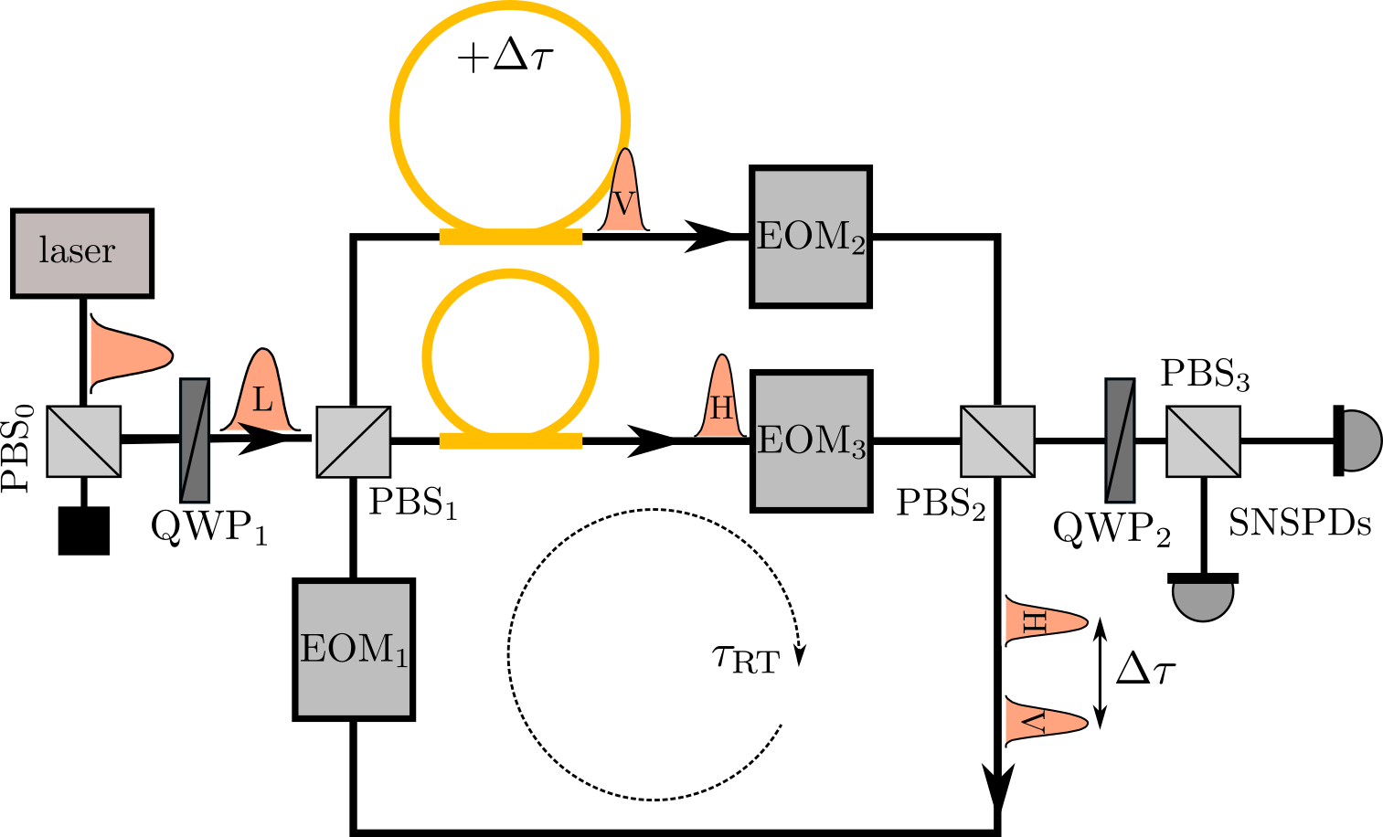
Simulator and experimental realization:—Fig. 1 shows the experimental setup for our quantum simulator. At its core is a Mach-Zehnder interferometer with a feedback loop realising the chiral translation , Eq. (2), via time-multiplexing: A laser pulse is split into horizontal and vertical polarization orientations (the ‘spin’-components ) and send through fiber lines of different lengths. In this way positions on the lattice are mapped onto time domain, with time delay between vertically/horizontally polarized pulses defining the lattice constant [13, 14, 15]. The network architecture offers full control over the dynamic coin operations , Eq. (3) via polarization rotations [14, 16], and allows to measure the spin resolved probability distributions defined in Eq. (4) [17]. It thus provides the key ingredients of our proposal. In the following, we discuss the concrete realization of this protocol in the quantum optical simulator. Readers primarily interested in results are invited to continue reading in the following section.
We realize the quantum walker by a weak coherent laser pulse at telecom wavelength and its polarisation acts as the internal degree of freedom. The initial polarisation is set at quarter wave plate QWP1 at -45∘, such that left circular light enters the setup. The dynamic coin operation is accomplished by an EOM, implementing the voltage dependent polarisation rotation
| (6) |
As the EOM switches fast enough to address each pulse (i.e. each quantum walk position) individually it is capable of realising both static and dynamic disorder. Its programmability makes the recording of hundreds of patterns in short time without manual setup of parameters possible. After the coin operation, the light pulses are split according to their polarisation at a polarising beam splitter (PBS1) and are routed into the two arms of the interferometer. The pulses propagating in the upper arm are retarded by a time delay of ns relative to those in the lower arm. The conditional routing of the photons through the long or short fibre realises the chiral translation operator, Eq. (2). The time delay and roundtrip time here define the lattice spacing and single time step duration, respectively. After PBS2 the pulses are feedbacked in the loop and the dynamics continues until the desired final step, in which the train of pulses is deterministically coupled out by the EOMs 2 and 3. Given that these EOMs flip the polarization for the in and outcoupling the full dynamics of an step evolution is described by
The application of the operator describes the first transition through the fibre arms in which the role of the horizontally and the vertically polarized light is swapped with respect to the following roundtrips. The consecutive matrices signify the polarization flip by the EOMs 2 and 3 for in and outcoupling. As commutes with and using we obtain for the full evolution
which satisfies the chiral symmetries introduced above.
The deterministic in- and outcoupling of the light, as already introduced in [15, 18], minimizes the roundtrip losses with respect to the probabilistic version used earlier [13] and thus enables the recording of longer dynamics. The detection units consists of two superconducting nanowire single photon detectors (SNSPDs) with dead times well below the pulse separation, which in combination with PBS3 and a QWP at enable the measurement of each pulse intensity in the circular basis.
Results:—We obtain the spin-resolved probability distribution by recording measurements for 500 different realisations of polarization rotations simulating the static binary disorder discussed above. To define a reference frame without Anderson localization to compare to, we additionally simulate dynamic disorder for which localization is absent due to the destruction of phase coherence. The latter is realized via application of the polarization rotations randomly distributed in time, at otherwise identical system parameters.
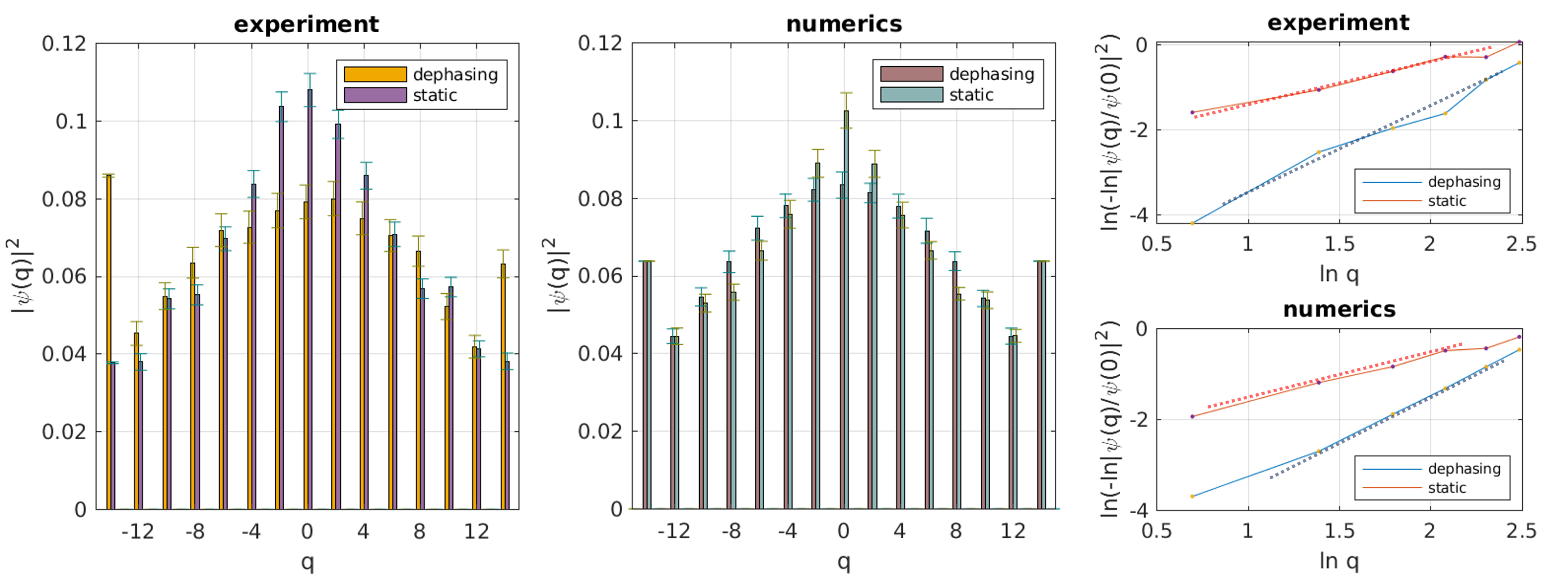
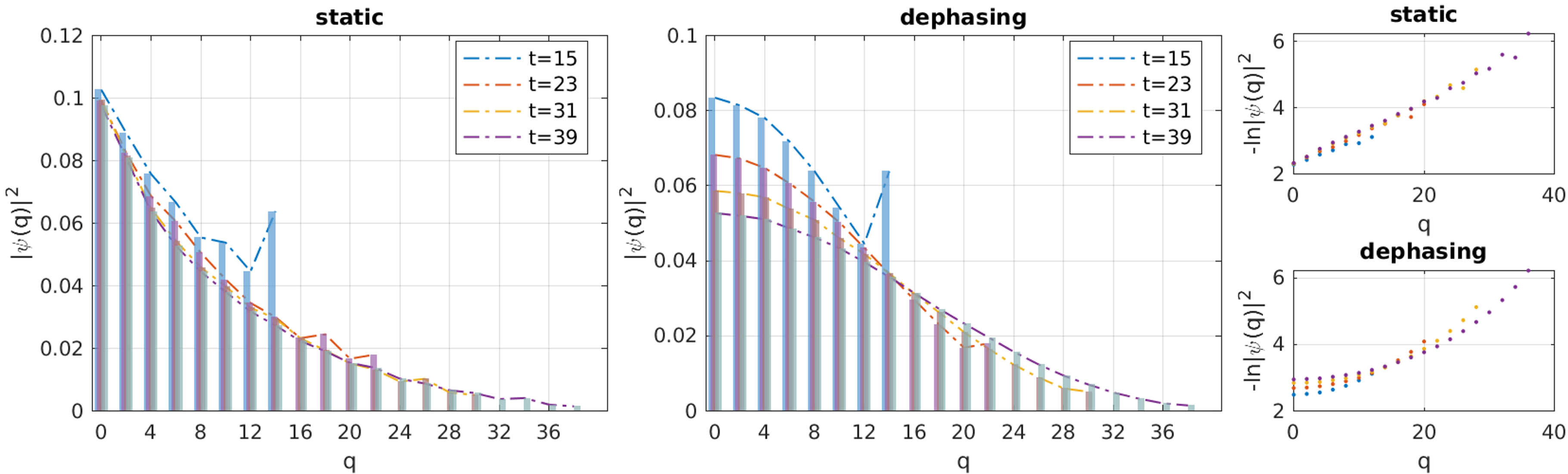
The comparison between the two recordings is presented in Fig. 2, at time step , traced over polarisation. At these values, the Anderson localized and the diffusively spreading wave package do not yet differ by much in absolute values. Instead, the difference shows in the shape of the distribution. That is, the convex profile of an exponential distribution in the Anderson localized case, compared to the concave form of a Gaussian diffusive profile, as verified in the right panel. (The boundary peaks in the diffusive case represent a small fraction of quasi-ballistically propagating contributions which disappear in the numerical simulation of longer runs, see Supplemental Material.)
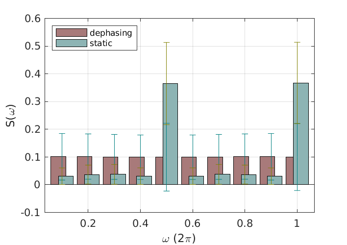
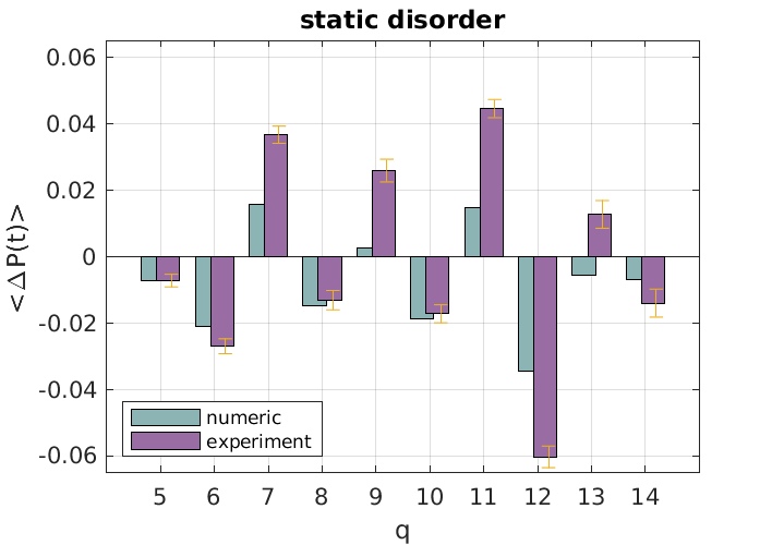
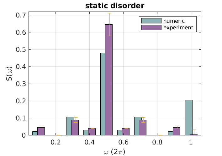
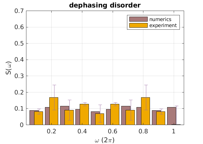
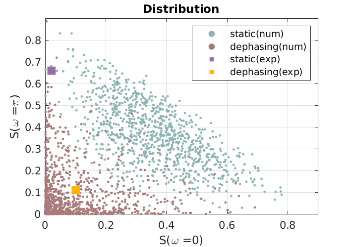
For each random realization of binary angles we extract the spatially integrated spin-polarization, Eq. (5), which we then average over different angle realizations. The upper left panel in Figure 3 shows experimental data, and corresponding numerical simulations, for between and 14 time steps, averaged over 500 realizations of static binary disorder. The upper-right panel exhibits the resulting power spectrum, , where . For comparison, we show in the lower left panel the corresponding power spectrum for dynamic binary disorder. The latter has a structureless random pattern with contributions of the same order from all frequencies, as expected for a noisy spin polarization. In contrast, the spin polarization for static disorder shows the time-staggering predicted for the topological quantum critical state, which is also witnessed by the pronounced peak at in the power spectrum. The relatively small number of time-steps probed in the experiment implies sizeable fluctuations of random parameters, which need to be taken into account in the interpretation of data: for a given run, the average value of randomly drawn angular parameters scales as , and a value of comparable magnitude for the staggered amplitude. In this way, the critical states both, at and get effectively gapped out for at least a fraction of the runs, resulting in a suppression of peaks in the power spectrum at and , respectively (cf. Fig. 3). To further illustrate this point, we repeated numerical simulations of ensembles of 500 random binary angle configurations a large number of times. In the right-lower panel of Fig. 3 we show the distributions of peak values in the power spectrum, resulting from 1000 repetitions of the previously described procedure. That is, each point here presents the average over an ensemble of 500 angle realizations (the ensembles used in experiment are indicated by the squares). As anticipated above, the distribution for static disordered is centered around large peak values, either at , at , or at both. The distribution for dynamic disorder, on the other hand, is always dominated by small peak values at both frequencies. The average power spectrum for the entire ensemble of angle configurations (cf. Supplemental Material) then shows the expected two-peak structure, with peaks at dominating over an otherwise approximately flat background, confirming thus that upon simulating larger runs, fluctuation effects diminish.
Conclusion:—We have realized an optical linear network simulator of one-dimensional topological quantum criticality. The simulator implements the photonic quantum walk of a spin-1/2 particle with chiral symmetry. Its optical network architecture allows us to fully access and monitor the state’s internal degree of freedom. Upon tuning to the critical point separating two topological Anderson insulating phases, we observe a time-staggered spin-polarization recently suggested as a smoking gun signature of quantum critical dynamics. Externally imposed time dependent noise, or ‘dephasing disorder’, destroys the signal, revealing its origin in quantum coherence. A similar destruction takes place upon breaking the chiral symmetry of the walk, and along with it the transition between two symmetry protected topological phases. Ideally, one would like to monitor scaling phenomena induced by such type of symmetry breaking, however, the currently realizable signal times are still too short for such type of statistics. Irrespective of such limitations, we believe that fully programmable quantum networks promise interesting perspectives for the simulation of topological quantum matter in the presence of engineered randomness.
Acknowledgements.
The Integrated Quantum Optics group acknowledges support by the ERC project QuPoPCoRN (Grant no. 725366). T. M. acknowledges financial support by Brazilian agencies CNPq and FAPERJ. A. A. and D. B. acknowledge partial support from the Deutsche Forschungsgemeinschaft (DFG) within the CRC network TR 183 (project grant 277101999) as part of projects A01 and A03. K.W.K. acknowledges financial support by Basic Science Research Program through the National Research Foundation of Korea (NRF) funded by the Ministry of Education (No.2021R1F1A1055797) and Korea government(MSIT) (No.2020R1A5A1016518).References
- Anderson [1958] P. W. Anderson, Absence of diffusion in certain random lattices, Phys. Rev. 109, 1492 (1958).
- Abrahams et al. [1979] E. Abrahams, P. W. Anderson, D. C. Licciardello, and T. V. Ramakrishnan, Scaling theory of localization: Absence of quantum diffusion in two dimensions, Phys. Rev. Lett. 42, 673 (1979).
- Evers and Mirlin [2008] F. Evers and A. D. Mirlin, Anderson transitions, Rev. Mod. Phys. 80, 1355 (2008).
- Altland et al. [2015] A. Altland, D. Bagrets, and A. Kamenev, Topology versus anderson localization: Nonperturbative solutions in one dimension, Phys. Rev. B 91, 085429 (2015).
- Balents and Fisher [1997] L. Balents and M. P. A. Fisher, Delocalization transition via supersymmetry in one dimension, Phys. Rev. B 56, 12970 (1997).
- Chabé et al. [2008] J. Chabé, G. Lemarié, B. Grémaud, D. Delande, P. Szriftgiser, and J. C. Garreau, Experimental Observation of the Anderson Metal-Insulator Transition with Atomic Matter Waves, Phys. Rev. Lett. 101, 255702 (2008).
- Hainaut et al. [2018] C. Hainaut, I. Manai, J.-F. Clément, J. C. Garreau, P. Szriftgiser, G. Lemarié, N. Cherroret, D. Delande, and R. Chicireanu, Controlling symmetry and localization with an artificial gauge field in a disordered quantum system, Nature Communications 9, 1382 (2018).
- Billy et al. [2008] J. Billy, V. Josse, Z. Zuo, A. Bernard, B. Hambrecht, P. Lugan, D. Clément, L. Sanchez-Palencia, P. Bouyer, and A. Aspect, Direct observation of Anderson localization of matter waves in a controlled disorder, Nature 453, 891 (2008).
- Bagrets et al. [2021] D. Bagrets, K. W. Kim, S. Barkhofen, S. De, J. Sperling, C. Silberhorn, A. Altland, and T. Micklitz, Probing the topological anderson transition with quantum walks, Phys. Rev. Research 3, 023183 (2021).
- Note [1] We have , and .
- Note [2] The associated topological invariants may be identified by analysis of the auxiliary ‘Hamiltonian’ . However, we will not need this underlying structure [19, 20] throughout.
- Note [3] To probe only critical states, one may prepare initial states extended over several sites with fixed phase relations, as discussed in Ref. [9]. Their experimental realization is, however, challenging and we thus focus on initial states localized on single sites, probing the entire quasi-energy spectrum.
- Schreiber et al. [2010] A. Schreiber, K. N. Cassemiro, V. Potoček, A. Gábris, P. J. Mosley, E. Andersson, I. Jex, and C. Silberhorn, Photons Walking the Line: A Quantum Walk with Adjustable Coin Operations, Phys. Rev. Lett. 104, 050502 (2010).
- Schreiber et al. [2011] A. Schreiber, K. N. Cassemiro, V. Potoček, A. Gábris, I. Jex, and C. Silberhorn, Decoherence and Disorder in Quantum Walks: From Ballistic Spread to Localization, Physical Review Letters 106, 180403 (2011).
- Nitsche et al. [2018] T. Nitsche, S. Barkhofen, R. Kruse, L. Sansoni, M. Štefaňák, A. Gábris, V. Potoček, T. Kiss, I. Jex, and C. Silberhorn, Probing measurement-induced effects in quantum walks via recurrence, Science Advances 4, eaar6444 (2018).
- Barkhofen et al. [2017] S. Barkhofen, T. Nitsche, F. Elster, L. Lorz, A. Gábris, I. Jex, and C. Silberhorn, Measuring topological invariants in disordered discrete-time quantum walks, Phys. Rev. A 96, 033846 (2017).
- Barkhofen et al. [2018] S. Barkhofen, L. Lorz, T. Nitsche, C. Silberhorn, and H. Schomerus, Supersymmetric polarization anomaly in photonic discrete-time quantum walks, Phys. Rev. Lett. 121, 260501 (2018).
- Nitsche et al. [2020] T. Nitsche, S. De, S. Barkhofen, E. Meyer-Scott, J. Tiedau, J. Sperling, A. Gábris, I. Jex, and C. Silberhorn, Local versus global two-photon interference in quantum networks, Phys. Rev. Lett. 125, 213604 (2020).
- Asbóth [2012] J. K. Asbóth, Symmetries, topological phases, and bound states in the one-dimensional quantum walk, Phys. Rev. B 86, 195414 (2012).
- Asbóth and Obuse [2013] J. K. Asbóth and H. Obuse, Bulk-boundary correspondence for chiral symmetric quantum walks, Phys. Rev. B 88, 121406 (2013).
Appendix A Probability distributions at longer times
As discussed in the main text, all states in the quasienergy spectrum contribute to the probability distribution of the walker. Since most of the states are non-critical, the probability distribution for static binary disorder thus follows , as shown in Fig. 4 (left panel) for numerical simulations of different time steps . The -dependence of is plotted in Fig. 4 (right-top panel), clearly showing a linear dependence on position. When the binary disorder also fluctuates in time, quantum phase coherence is destroyed turning dynamics thus into classical diffusion, , with . The numerical simulation, Fig. 4 (center and right-bottom panel), confirms the diffusive behavior and corresponding scaling of . Notice that the boundary peaks in the probability distributions are due to a small fraction of quasi-ballistically propagating states. As shown in Fig. 4, their contribution disappears as longer times are probed.
Appendix B Statistics of the power spectrum
The relatively small number of time steps measured in the experiment implies that the signature of critical states, viz. the time-staggered spin polarization, is subject to large statistical fluctuations. From our numerical simulations we find that it is necessary to average over many more than 500 disorder realizations to clearly observe the two-peak structure in the power spectrum. Figure 3 (bottom-right panel) in the main text shows the distribution of 1000 peak heights at frequencies in the power spectrum for static (purple) and dephasing disorder (blue). Each of the 1000 shown points is obtained from averaging the power spectrum over 500 random disorder realizations. The average and standard deviation of the entire power spectrum after averaging over the total ensemble of realizations is plotted in Fig. 5 below.