Experimental Demonstration of Swift Analytical Universal Control over Nearby Transitions
Abstract
Along with the scaling of dimensions in quantum systems, transitions between the system’s energy levels would become close in frequency, which are conventionally resolved by weak and lengthy pulses. Here, we extend and experimentally demonstrate analytically based swift quantum control techniques on a four-level trapped ion system, where we perform individual or simultaneous control over two pairs of spectrally nearby transitions with tailored time-varied drive, achieving operational fidelities ranging from 99.2(3)% to 99.6(3)%. Remarkably, we achieve approximately an order of magnitude speed up comparing with the case of weak square pulse for a general control. Therefore, our demonstration may be beneficial to a broad range of quantum systems with crowded spectrum, for spectroscopy, quantum information processing and quantum simulation.
Despite frequent utilization of two-level systems for many quantum enhanced applications, most practical systems are intrinsically of many levels nature, whose energy separations come from couplings of internal degrees of freedom or from splittings by external fields. Besides, for applications with quantum many-body system, such as, high-sensitivity precision measurements [1], large-scale quantum computation [2] and simulation of quantum many-body system [3], either more qubits or larger internal complexities must be involved, and then the energy or associated frequency spectrum would become crowded. In these cases, spectrally resolving a transition with an external drive field for high-fidelity manipulation would become difficult, which may limit the scalability of quantum systems, and may hinder large-scale quantum tasks where precise quantum control over individual transition is required.
A straightforward solution for this limitation is to narrow the range of Fourier frequency components from the pulse of the drive field, for example to apply smooth-shaped pulses [4, 5, 7, 6, 8] and using narrow linewidth transitions [9]. However, in general cases, a desired transition rate determines the minimum temporal integral of pulse strength, i.e. “pulse area”, and the lower field strength in turn results in longer pulse duration, leaving the control vulnerable to frequency drifts, decoherence or limiting the number of operations in given finite coherence times. Meanwhile, insufficiently weak pulse strength would create unwanted transition in the adjacent spectral line, giving rise to a population leakage or cross-talk error in the control.
To tackle with the problem of spectral crowding while keeping the operation fast, one idea is to abandon the assumption that the unwanted nearby transitions remain without being driven, but rather allowing a controlled evolution where the overall desired operation is reached at the end of the drive pulse. By numerically searching for desired pulse shape with optimal control techniques [10, 11, 12, 13, 14, 15], an overall operation close enough to the target one can be obtained. However, the numerical pulse shaping can only be done in a case-by-case way, and only one certain shape can be obtained under a particular set of conditions. Besides, due to the piecewise constant control ansatz, the complex numerical shape may be inaccurate in cases of bounded bandwidth.
On the other hand, for two-level quantum systems, analytic solution for detuned single or multiple axis driving become available [16, 17, 18]. This brings an opportunity to better understand the underlying physics, and converting a full numerical optimization to a parametric boundary problem, where a series of solutions can be obtained when the boundary conditions are met. Thus, one has the additional freedom to incorporate various pulse-shaping techniques, and find experimental-friendly simple pulse solutions. We note that this analytic solution can be extended to drive desired transitions in multi-level quantum systems, while leaving adjacent transitions intact. Therefore, such a technique can go beyond addressing a certain transition, and can be tailored to simultaneously drive nearby transitions. The combination of individual and simultaneous control would lead to the capability of arbitrary manipulations in the nearby transitions, and may assist in quantum logic operations on multi-level systems [19, 20, 7, 21, 22, 23, 24, 25]. Remarkably, as this technique removes the weak drive limitation, it might be also useful for spectroscopy, where a faster probe to obtain more information might be possible.
Here, we extend these analytical based swift quantum control techniques to a four-level system, where individual or simultaneous quantum control over the two pair of levels can be effectively obtained. We then experimentally demonstrate individual operation where a transition is driven while the other is intact, and simultaneous operations where quantum phase and Hadamard gate operations are performed on both transitions. We achieve operation fidelities ranging from 99.2(3)% to 99.6(3)%, limited by decoherence and experimental imperfections.
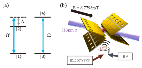
We firstly extend previous two-level schemes [16, 17, 18] to the case of four levels forming two pairs of nearby transitions, as shown in Fig. 1(a), to implement a fast, high-fidelity universal control over the two transitions. Labeling the transition frequency between as , when the transition with is driven resonantly by an external field with time-varied Rabi rate , the transition with is driven simultaneously by the same field with Rabi rate with detuning from resonance. Here we consider the case that and with a fixed ratio; the transition frequencies across the two pairs are much larger than or , thus we can limit our discussion within each pair. In the rotating framework, we obtain the interacting Hamiltonian as
| (1) |
where is the phase of drive field. Thus, the nearby small detuned transition will be excited unintentionally, leading to phase and leakage errors, i.e., the so-called spectral crowding problem. The trivial way to deal with the problem is to drive the target transitions with a lower Rabi rate, i.e., max, typically with max for a general control. However, lower Rabi rates lead to longer control time and less number of control pulses within the coherence times. As we analyze and experimentally demonstrate below, the time-dependent control in this work would enable individual or simultaneous control of both transitions even with max, thus giving approximately an order of magnitude speed up.
To illustrate the idea for swift analytic-based control, we consider the general evolution operator of Hamiltonian in Eq. (33) with a duration as
| (2) |
where and are the evolution operator for the resonant and detuned subspace, respectively. To obtain precise control over the transitions, we need to obtain target dynamics for both subspaces, preferably beyond the weak drive limit. While the evolution in the resonant subspace is related to the pulse area and phase given by in Eq. (33) in a straightforward way, the complex dynamics of the detuned subspace can be obtained, by extending Refs. [16, 17, 18], as [26]
| (3) |
where is
| (6) |
and with
| (9) |
which is parameterized by , and . This analytic solution allows us to achieve any SU(2) matrix, and the required is determined by and as
| (10) |
Thus it is possible to design for arbitrary control in the detuned subspace. For the resonant subspace, given a fixed value of , Eq. (10) leads to a waveform of for a controlled rotation; concatenated segments with varied give arbitrary control [26]. To obtain , we can further decompose into a weighted sum of analytic functions, e.g., sinusoidal functions, with a period equal to the total operation time , and we can numerically find proper weights to obtain a required overall operation at , under further constrains of and being finite. In practice, we set , then and are on the order of and , respectively. Thus in general the two terms in Eq. (10) are both on the order of and are not canceled with each other, so that the average of Rabi rates can be roughly on the order of , and the operation time is much shorter than the weak driven case.
In our experiment, we trap a ion in a linear Paul trap [28] as shown in Fig. 1(b), and the desired Hilbert space is defined within the hyperfine states of the ion, with , , and . Applying an ambient magnetic field at 6.7798 mT, we have MHz, MHz, kHz, and . We apply radio-frequency (RF) fields driving transitions and . RFs are generated by an arbitrary-wave-generator (AWG) with a power amplifier [26], and thus can be fully controlled by programming the AWG. When we drive the transition on resonance with Rabi rate , the transition is also driven with Rabi rate and a detuning , thus implementing the Hamiltonian in Eq. (33). The Rabi rate ratio is experimentally measured to be 1.7, and remains fixed throughout the experiment since it depends on the coupling constants. To assist state preparation and detection, we also apply microwave fields to a separate antenna, as shown in Fig. 1(b), sourced by a power amplified frequency-doubled direct-digital-synthesizer.
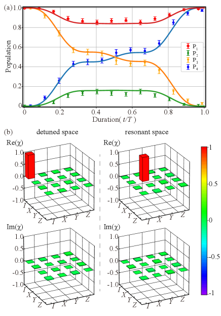
As a demonstration of individual control over one of the two closely spaced transitions, while leaving the other intact, we perform a simultaneous operation on both pairs of transitions with and (), where is a Pauli operator and is an identity operation. According to Eq. (10), we can obtain from and , where we set
| (11) |
with , leading to , thus , and . When we design a specific waveform, we can set the boundary conditions and find parameters by numerical optimization with trust-region-dogleg method [29]. By setting s for 81 kHz and with numerical optimization, we obtain respectively, giving . Thus the average of Rabi rates =56 kHz and = 33 kHz, comparable to . The quantum dynamics is shown in Fig. 2 (a), where the solid lines are obtained by theoretical simulation while the points are the experimental results. The quantum process can be described by , where is the density matrix of the initial state, is the density matrix of the state after the process, are basis operators, is the identity operation, and , and represent Pauli operators. Thus the matrix uniquely represents the process. To estimate the components of for the operation, we perform process tomography [30, 31, 32], where we initialize the ion to various states, apply the operation, and measure the outcome. For example, to measure components of , we first apply Doppler cooling, optical pumping with 313 nm laser pulses [26] to prepare state, and apply resonant microwave or pulses to transfer to states of , , and , respectively. After applying the operation, we map one state in the pair to and the other to by a series of microwave pulses, followed by resonant fluorescent measurement by driving to for 400 , while the state is out of resonance and appears dark. We typically collect on average 25 counts for and less than 1 count for dark states. We perform each measurement for 1000 trials to reconstruct by maximum likelihood state tomography [33, 6, 34], and from which we further obtain the process matrix components, as shown in Fig. 2 (b). Similar procedure is repeated to measure components of . We obtain process fidelity [30, 35] and , respectively, through the definition of
| (12) |
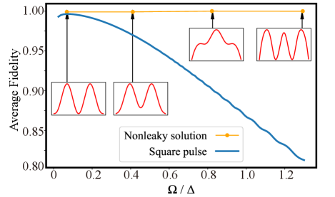
where is the ideal process matrix for the corresponding operation and is the measured one. In our experiment, the measured coherence times for the resonant and detuned subspaces are approximately 1.9 ms and 1.1 ms, respectively, with Ramsey type experiment, which will contribute up to approximately 0.2% operation infidelity. Experimentally, we also observe fast drifts of the ambient magnetic field after each calibration, which, together with other unknown ones, we attribute as other possible error sources. Finally, to compare with the case of weak square pulse, we performed a numerical simulation [26]. Given a realistic decoherence of and as in the experiment and without further imperfections, the optimal control fidelity with square pulse is reached at , while for our implementation a similar fidelity can be achieved at , and thus decrease the required operation time by approximately an order of magnitude.
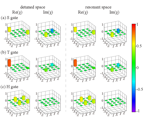
We next demonstrate simultaneous quantum control over both pairs of transitions, by implementing as quantum logic gates of S gate, T gate and Hadamard (H) gate [26], in a two-step way with their corresponding manipulation times being and , respectively, so that the total gate-time is . In the phase gate cases, a rotation around the axis with angle is applied in both detuned and resonant subspaces, where , for S and T gates, respectively, by setting . According to Eq. (11), we can obtain specific parameters for in Eq. (10). Then, we can apply two waveforms similar to Eq. (11) with different initial phase for the two steps to construct a desired phase gate, leading the first step to and with the initial phase of the pulse being , and for the second step and with the initial phase being . In this way, we can get . As for H gate, in the first step, we set , in Eq. (11) and optimize to obtain , which lead to and , and for the second step, we can apply a waveform that is the same as the individual control in Eq. (11) with , to get and . The two operations form . We design waveforms with gate time s respectively for each gate, similar to the process above and perform process tomography, with details in supplemental material [26]. The process matrices are shown in Fig. 3, with process fidelity = 99.4(3)%, = 99.4(3)%, = 99.3(3)%, = 99.4(4)%, = 99.2(2)% and = 99.2(3)%, where and correspond to S, T and H gates on the detuned and resonant transitions, respectively.The decoherence affects the measured fidelity with a contribution up to approximate 0.3%, 0.3% and 0.4% for S, T and H gates, respectively.
In conclusion, we experimentally demonstrate quantum control over two pairs of nearby transitions with time-dependent pulses, where the waveform parameters can be readily obtained with the help of an analytical model. We demonstrate individual and simultaneous control of each pair of transitions, reaching a process fidelity up to 99.6(3)%. Our work can be extended to a range of systems. For example in recent experiments with trapped molecular ions, adjacent transitions can be spaced on the order of kHz, rendering the transition pulse duration on the order of ms with smooth edges [7]; and for long ion chain, coupled motional modes can space below 10 kHz [19, 25] and superconducting transmon qubits with weak anharmonic levels [20]. For future research, it might be interesting to enhance the robustness for the designed shaped pulses or even incorporate optimization requirements into the process of finding a target solution [36]. In addition, as more levels may be involved for many-body or many-degree-of-freedom quantum systems, extending the current mathematical model to cover more levels that are closely spaced may be also of practical interest. On the other hand, our demonstration involves four levels orthogonal to each other, thus some extension would be needed when the transitions involve a shared energy level, such as -, V-, and ladder-type systems. Regarding quantum sensing and metrology, this demonstration might be beneficial to vector magnetometry utilizing nitrogen-vacancy centers [37] to produce a fast probe driving nearby transitions corresponding to a few crystal orientations.
Acknowledgements.
We thank Pengfei Wang and Xinhua Peng for helpful discussions. We acknowledge support from the National Natural Science Foundation of China (grants No. 92165206, No. 11974330 and No. 11874156), the Chinese Academy of Sciences (Grant No. XDC07000000), Anhui Initiative in Quantum Information Technologies (Grant No. AHY050000), and the Fundamental Research Funds for the Central Universities.I Supplemental Material
II Exact solution and speed-up comparing with square pulse
We here expand the analytical solution in Refs. [17, 18] to a general form. The Hamiltonian for a two-level quantum system that is driven by a classical field in a detuned way is
| (15) |
where is the detuning between the transition frequency and the driving field frequency, with and being the amplitude and phase of the driving field, respectively. To get the solution, we first apply a rotation around the vertical axis of axis in x-y plane, denoted as , and the Hamiltonian will be changed to
| (18) |
Generally, the corresponding time evolution operator for the above Hamiltonian can be written as
| (21) |
with .
In the rotating framework of , the Schrödinger equation of the evolution operator will change to
| (22a) | |||
| (22b) | |||
where
and Combining two terms, we get
| (23) |
then we separate the left part as two different equation of , . And the right part would also be separated with a complex parameter , i.e., , which respect to the Schrödinger equation from. By solving these separated differential equations, ones can get
| (24a) | |||
| (24b) | |||
here, the complex function is unknown yet. Here and are constant phases which are hidden in the derivation. Meanwhile, we can also denote in terms of as
| (25) |
where . As and are real, the function defined by them also should be a real function, which allows us to derive the relationship between the real and imaginary parts of . Thus, the real and imaginary parts of is obtained as
| (26a) | |||
| (26b) | |||
where , and is an integral constant.
By applying , the picture will return back to the one respects to , Then, the time evolution operator can be calculated as
| (29) |
where and Here we have also set for a simplicity, but in general, this constant phase can be arbitrary, as we discuss below. Besides, we also set to simplify our calculation. Then the amplitude of the driving field can be obtained as
| (30) |
Due to the practical restriction of the pulse shape, the function should be chosen so that and are finite. Besides, to be more experimental-friendly, we also set .
Furthermore, considering the boundary condition must be met for any , we set the operator with the form of
| (31) |
Note that, the unknown constant phases and would be canceled themselves in the calculation lead to the operator under this assumption, as been verified by our numerical simulation and experiment. Finally, turning back to original frame, the analytical solution of the time evolution operator is
| (32) |
We did numerical simulations to compare the performance between using swift analytical control and using square pulses, aiming to conduct the individual control. The Hamiltonian of our system is
| (33) |
We can design the Rabi rate so that , where is the operation duration, then we can get a rotation on the resonant subspace, without any restriction on the pulse shape. Meanwhile, the nearby small detuned transition can be driven simultaneously, by tuning the pulse shape to meet the form in Eq. (30), we can get any target operator in this subspace. We simulate the effect of the unintentional drive as shown in Fig. 4. We define the operator fidelity between the unintentional drive and , where is the identity operation. We did the simulation with the dephasing rate being and . Our analytical solution based pulse can keep good fidelity(%) even with increasing .
III Universal quantum control
Firstly, we focus on individual control (ID) over one of the two closely spaced transitions. For this purpose, we can perform an target operation on the resonant subspace, e.g., , while maintain the integrity of the detuned subspace, i.e., , where is a Pauli operator and is an identity operation. Then, the exemplified operator is
To realize this operation, in the resonant subspace, a simple pulse is enough. And, in the detuned subspace, the analytic solution in Eq. (32) shows that the evolution operator can be written as
where we have set , and assumed for simple calculation. These settings lead to
And the function in experiment is set as
| (34) |
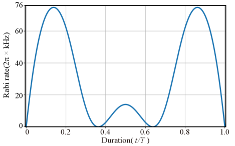
where are arbitrary parameters to be determined by various purpose. Here, we choose to satisfy and to make sure . The rest of could be used to determine the value of numerically, providing different possible gate series. Here, we choose and to implement the target individual control with short operational time, and the resulted pulse shape is shown in Fig. 5.
In principle, arbitrary control over each subspaces can be obtained. Therefore, besides the individual control, we also present how to implement simultaneously quantum gates, such as S gate, T gate and Hadamard (H) gate on both subspaces. For a qubit system, these gates form a universal set of single-bit gates In the case S gate, it denotes a rotation around axis in both detuned and resonant subspace,i.e.
To implement this single-bit gate, we need two pulse with different . In the resonant subspace, we set
| (35a) | |||
| (35b) | |||
So the gate was implemented. For detuned subspace, recall the analytic solution, we find the phase in evolution operator is independent on of the drive field, thus the phase in these two pulses are actually equal, and the final operator is
When , ones implement the gate , so the S gates in two subspace is obtained. The amplitudes for both steps of the waveform designed for S gate are the same with and s. As for T gates, just set , it can be implemented in a similar way. The waveform parameters designed for T gate are and s.
We now consider the Hadamard (H) gate for both subspaces, that is,
To implement the gate in resonant subspace, we decompose H gate as , where denote the Pauli matrix , which could be obtained by a resonant pulse with different phase with the pulse area being . Thus, we set
| (36a) | |||
| (36b) | |||
For the detuned subspace, we implement an identity in the first part of evolution, and an H gate for the second part. The corresponding restriction of parameter in second part is , and the second part of the waveform is designed with parameters and s. Similar as before, the H gate could be implemented with accurately calculated with .
IV Experimental result
The data of matrix for individual or simultaneous control is shown as follows, in each of the subspaces. correspond to the individual control, simultaneous S, T and H gates process matrix for resonant space; is the process matrix for detuned space, with and representing the real and imaginary components respectively:
| (37) |
| (38) |
| (39) |
| (40) |
| (41) |
| (42) |
| (43) |
| (44) |
| (45) |
| (46) |
| (47) |
| (48) |
| (49) |
| (50) |
| (51) |
| (52) |
V Details of Experiment hardware
We use commercial 313 nm laser sources from Precilasers Co. Ltd. (YEFL-FHG-313-0.3-CW), frequency locked to reference spctral lines of molecular iodine with a home-built saturation spectroscopy setup via the 626 nm monitor output. We use commercial AWG from Ciqtek (AWG4100). The AWG is triggered and synchronized with home-developed board and user interface (based on and modified from [27]), which control direct-digital-synthesizer and Transistor-transistor logic for other pulses and record photon counts during fluorescent detection. The power amplifiers used for RF and microwave fields are Mini Circuits ZHL-100W-GAN+ and ZHL-30W-252-S+ respectively. The maximum power we use for RF and microwave fields are 50 W and 30 W respectively. We set two separate antennas for RF drive and microwave drive, about 2 cm away from the ion. The RF antenna has a shape of a coil with around 3 cm diameter made from a single turn of copper wire. A 100 nH inductor and a 30 pF capacitor in parallel with the coil improve the coupling of the radio frequency to the antenna. The microwave field is delivered through a twin spiral antenna with a diameter of around 3 cm.
References
- [1] V. Giovannetti, S. Lloyd, and L. Maccone, Science 306, 1330 (2004).
- [2] A. Blais, A. L. Grimsmo, S. M. Girvin, and A. Wallraff, Rev. Mod. Phys. 93, 025005 (2021).
- [3] C. Monroe, W. C. Campbell, L.-M. Duan, Z.-X. Gong, A. V. Gorshkov, P. W. Hess, R. Islam, K. Kim, N. M. Linke, G. Pagano, P. Richerme, C. Senko, and N. Y. Yao, Rev. Mod. Phys. 93, 025001 (2021).
- [4] L. M. K. Vandersypen and I. L. Chuang, Rev. Mod. Phys. 76, 1037 (2005).
- [5] C. J. Ballance, T. P. Harty, N. M. Linke, M. A. Sepiol, and D. M. Lucas, Phys. Rev. Lett. 117, 060504 (2016).
- [6] J. P. Gaebler, T. R. Tan, Y. Lin, Y. Wan, R. Bowler, A. C. Keith, S. Glancy, K. Coakley, E. Knill, D. Leibfried, and D. J. Wineland, Phys. Rev. Lett. 117, 060505 (2016).
- [7] C.-w. Chou, C. Kurz, D. B. Hume, P. N. Plessow, D. R. Leibrandt, and D. Leibfried, Nature 545, 203 (2017).
- [8] Y. Lin, D. R. Leibrandt, D. Leibfried, and C.-w. Chou, Nature 581, 273 (2020).
- [9] D. Hayes, D. Stack, B. Bjork, A. C. Potter, C. H. Baldwin, and R. P. Stutz, Phys. Rev. Lett. 124, 170501 (2020).
- [10] F. Motzoi, J. M. Gambetta, P. Rebentrost, and F. K. Wilhelm, Phys. Rev. Lett. 103, 110501 (2009).
- [11] A. M. Forney, S. R. Jackson, and F. W. Strauch, Phys. Rev. A 81, 012306 (2010).
- [12] J. M. Gambetta, F. Motzoi, S. T. Merkel, and F. K. Wilhelm, Phys. Rev. A 83, 012308 (2011).
- [13] F. Motzoi and F. K. Wilhelm, Phys. Rev. A 88, 062318 (2013).
- [14] P. Rebentrost and F. K. Wilhelm, Phys. Rev. B 79, 060507(R) (2009).
- [15] S. Kirchhoff, T. Keßler, P. J. Liebermann, E. Assémat, S. Machnes, F. Motzoi, and F. K. Wilhelm, Phys. Rev. A 97, 042348 (2018).
- [16] E. Barnes and S. Das Sarma, Phys. Rev. Lett. 109, 060401 (2012).
- [17] E. Barnes, Phys. Rev. A 88, 013818 (2013).
- [18] S. E. Economou and E. Barnes, Phys. Rev. B 91, 161405(R) (2015).
- [19] S.-L. Zhu, C. Monroe, and L.-M. Duan, Phys. Rev. Lett. 97, 050505 (2006).
- [20] M. J. Peterer, S. J. Bader, X. Jin, F. Yan, A. Kamal, T. J. Gudmundsen, P. J. Leek, T. P. Orlando, W. D. Oliver, and S. Gustavsson, Phys. Rev. Lett. 114, 010501 (2015).
- [21] J. Randall, A. M. Lawrence, S. C. Webster, S. Weidt, N. V. Vitanov, and W. K. Hensinger, Phys. Rev. A. 98, 043414 (2018).
- [22] P. J. Low, B. M. White, A. A. Cox, M. L. Day, and C. Senko, Phys. Rev. Res. 2, 033128 (2020).
- [23] Y. Wang, Z. Hu, B. C. Sanders, and S. Kais, Front. Phys. 8, 589504 (2020).
- [24] M. Ringbauer, M. Meth, L. Postler, R. Stricker, R. Blatt, P. Schindler, and T. Monz, arXiv preprint arXiv:2109.06903 (2021).
- [25] Q. Mei, B. Li, Y. Wu, M. Cai, Y. Wang, L. Yao, Z. Zhou, and L. Duan, arXiv preprint arXiv:2110.03227 (2021).
- [26] See supplemental material for derivations of important formulas, example comparison in efficiency between our work and square pulse, detailed parameters and data analysis for the experiments, experimental setup and experiment hardware, which include [17, 18, 27].
- [27] C. Langer, High fidelity quantum information processing with trapped ions, Ph.D. thesis, Department of Physics, University of Colorado, Boulder (2006).
- [28] D. Leibfried, R. Blatt, C. Monroe, and D. Wineland, Rev. Mod. Phys. 75, 281 (2003).
- [29] A. R. Conn, N. I. M. Gould, and P. L. Toint, Trust Region Methods (Society for Industrial and Applied Mathematics, 2000).
- [30] J. Zhang, A. M. Souza, F. D. Brandao, and D. Suter, Phys. Rev. Lett. 112, 050502 (2014).
- [31] M. Riebe, K. Kim, P. Schindler, T. Monz, P. O. Schmidt, T. K. Körber, W. Hänsel, H. Häffner, C. F. Roos, and R. Blatt, Phys. Rev. Lett. 97, 220407 (2006).
- [32] M. A. Nielsen and I. L. Chuang, Quantum Computation and Quantum Information: 10th Anniversary Edition (Cambridge University Press, 2010).
- [33] A. C. Keith, C. H. Baldwin, S. Glancy, and E. Knill, Phys. Rev. A 98, 042318 (2018).
- [34] C. R. Clark, H. N. Tinkey, B. C. Sawyer, A. M. Meier, K. A. Burkhardt, C. M. Seck, C. M. Shappert, N. D. Guise, C. E. Volin, S. D. Fallek, H. T. Hayden, W. G. Rellergert, and K. R. Brown, Phys. Rev. Lett. 127, 130505 (2021).
- [35] X. Wang, C.-S. Yu, and X.X. Yi, Phys. Lett. A 373, 58 (2008).
- [36] A. Soare, H. Ball, D. Hayes, J. Sastrawan, M. C. Jarratt, J. J. McLoughlin, X. Zhen, T. J. Green, and M. Biercuk, Nat. Phys. 10, 825 (2014).
- [37] P. Wang, Z. Yuan, P. Huang, X. Rong, M. Wang, X. Xu, C. Duan, C. Ju, F. Shi, and J. Du, Nat. Commun. 6, 6631 (2015).