Experimental 3-dimensional tracking of the dynamics of a single electron in the Fermilab Integrable Optics Test Accelerator (IOTA)
Abstract
We present the results of experimental studies on the transverse and longitudinal dynamics of a single electron in the IOTA storage ring. IOTA is a flexible machine dedicated to beam physics experiments with electrons and protons. A method was developed to reliably inject and circulate a controlled number of electrons in the ring. A key beam diagnostic system is the set of sensitive high-resolution digital cameras for the detection of synchrotron light emitted by the electrons. With 60–130 electrons in the machine, we measured beam lifetime and derived an absolute calibration of the optical system. At exposure times of 0.5 s, the cameras were sensitive to individual electrons. Camera images were used to reconstruct the time evolution of oscillation amplitudes of a single electron in all 3 degrees of freedom. The evolution of amplitudes directly showed the interplay between synchrotron-radiation damping, quantum excitations, and scattering with the residual gas. From the distribution of measured single-electron oscillation amplitudes, we deduced transverse emittances, momentum spread, damping times, and beam energy. Estimates of residual-gas density and composition were calculated from the measured distributions of vertical scattering angles. Combining scattering and lifetime data, we also provide an estimate of the aperture of the ring. To our knowledge, this is the first time that the dynamics of a single electron are tracked in all three dimensions with digital cameras in a storage ring.
1 Introduction
Observation of a single electron in storage rings has a long history that goes back to experiments at AdA, the first electron-positron collider [1, 2]. Observation of discrete steps in radiation intensity offers unique metrology capabilities associated with the absolute calibration of circulating currents and radiation properties [3, 4, 5]. Another set of experiments was focused on measurements of synchrotron oscillations by registering deviations of photon arrival times with respect to the revolution reference signal [6, 7, 8]. A decade ago, advancements in digital imaging technology allowed experimenters to obtain digital images of radiation from single circulating electrons, but exposure times were too long to resolve and track instantaneous oscillation amplitudes [9].
This paper presents the results of a first series of experiments dedicated to a systematic study of an electron’s dynamics in the longitudinal and transverse planes by analyzing high-resolution digital images obtained with sensitive cameras. The experiments were carried out in March 2019 during IOTA Run 1. Studies on the precise measurement of photon arrival times will be presented separately.
Section 2 of this paper briefly describes the IOTA storage ring. Sections 3 and 4 cover the amplitude reconstruction method and the statistical properties of the observed parameters. Section 5 presents the experimental results: the evolution in time of the amplitude of an electron’s trajectory; single particle emittances and damping times; the lifetime of a beam with about 100 electrons; description of residual gas properties; and an estimate of ring acceptance. The last section (Section 6) concludes the paper with a summary and discussion of the main results.
2 The IOTA Storage Ring
The Integrable Optics Test Accelerator (IOTA) was recently commissioned with 100 MeV/ electrons as part of the Fermilab Accelerator Science and Technology (FAST) facility [10, 11]. IOTA is a storage ring with a circumference of 40 m (Figure 1). It can store electron or proton beams at momenta between 50 and 150 MeV/ and it can be reconfigured to accommodate different experiments. The main goal of IOTA is to demonstrate the advantages of nonlinear integrable lattices for high-intensity beams and to demonstrate new beam cooling methods [12, 10].


Low-emittance and highly configurable electron bunches are injected from the FAST superconducting linac [13, 14]. Electrons are extracted from a photo-cathode in a warm RF-gun immersed in a configurable longitudinal magnetic field. After that, the beam is accelerated by two TESLA-type superconducting cavities and one ILC-style cryomodule up to a kinetic energy of 300 MeV. Transverse steering and focusing of the beam are done with warm iron-based magnets. The FAST linac is equipped with a wide variety of beam diagnostics, including electrostatic pickups, YAG screens and optical transition radiation (OTR) foils.
During IOTA design and construction, special attention was given to beam diagnostics. The main set consists of the following components:
-
•
wall-current monitors (WCMs)
-
•
direct-current current transformers (DCCTs)
-
•
21 electrostatic pickups (BPMs)
-
•
2 synchrotron-radiation photomultipliers (PMTs)
-
•
8 synchrotron-radiation cameras
Precise beam position and shape measurements are necessary to tune IOTA lattice parameters to the required level [15]. It turns out that the sensitivity of the cameras is high enough to provide images even for a single electron circulating in the ring for relatively short exposure times (fractions of a second).
| Parameter | Value |
|---|---|
| Perimeter | 39.96 m |
| Momentum | 100 MeV/ |
| Electron current | 0–4.8 mA |
| RF frequency | 30 MHz |
| RF voltage | 250 V |
| Betatron tunes, () | (0.28, 0.31) |
| Synchrotron tune, | |
| Damping times, () | (6.15, 2.38, 0.91) s |
| Horizontal emittance (geom., RMS), | 36.6 nm |
| Momentum spread (RMS), | |
| Momentum compaction | 0.077 |


During the experiments presented in this paper, IOTA operated with 100 MeV electrons and was configured for experiments with one special nonlinear insertion, either a string of nonlinear Danilov-Nagaitsev magnets [12, 16] or an octupole channel to generate a Hénon-Heiles potential [17, 18]. Table 1 lists the beam parameters at the time of the experiments. Figure 2 shows the horizontal and vertical beta functions and Figure 3 shows the horizontal dispersion. The lattice parameters were analyzed and tuned using the LOCO technique [19, 20, 21]. The slight asymmetry in the lattice functions arises from the gradients in the main dipoles, which were compensated by the quadrupoles.
2.1 Synchrotron-Light Detection
Each of the 8 main dipoles in IOTA is equipped with synchrotron light stations installed on top of the magnets themselves. The light out of the dipoles is deflected upwards and back to the horizontal plane with two 90-degree mirrors. After the second mirror, the light enters the dark box, which is instrumented with customizable diagnostics, as shown in Figure 4. Custom 3D-printed viewport adapters and 2-inch black tubes are used to connect optical components and ensure light tightness. A focusing lens with a 40 cm focal length is installed in the vertical lens tube that connects to the mirror holders. At the time of the experiment, 7 magnets were equipped with sensitive digital cameras. The main characteristics of the cameras are listed in Table 2.

| Parameter | Value |
|---|---|
| Manufacturer | Point Grey (now FLIR) |
| Model | BFLY-PGE-23S6M-C |
| Resolution | 1920 1200 pixels |
| Sensor | Sony IMX249, CMOS |
| Pixel size | |
| ADC depth | 12 bit |
| Gain range | 0 to 29.996 dB |
| Exposure range | to 32 s |
| Temporal dark noise (read noise) | 7.11 |
| Saturation capacity (well depth) | 33106 |
| Quantum efficiency at 500 nm | 83% |
A single 100 MeV electron circulating in the IOTA ring produces about 7 500 detectable photons per second per main dipole [22], as confirmed by measurements with the photomultipliers. This intensity is enough to be easily detected by a PMT or by a sensitive digital camera. In IOTA, both PMTs and cameras are routinely used to study beams with intensities from a single electron up to the maximum current. About 10 photons per pixel are necessary to exceed the background noise level on our cameras. This puts a limit on the size of the light spot at the camera sensor.
3 Amplitude Reconstruction Method
The oscillation amplitudes of the electron trajectories were obtained by comparing synchronized sets of images with a model describing the expected projections of these images onto the horizontal and vertical axes.
The scaling factors for each camera were based on closed-orbit responses of both cameras and electrostatic pickups to dipole trims and RF frequency modulation, using the LOCO technique. A precise modulation of the RF frequency allowed us to get an absolute calibration from the dispersion measurements. This resolved calibration degeneracies in the LOCO data set and gave absolute calibrations for both BPMs and trims.
There are several known effects that affect images quality. The first group blurs an image and includes aberrations, diffraction, vignetting and finite depth of field of the optics that images part of a curved trajectory. There is also a possibility of nonlinear distortions. After thorough alignment linearity and absence of vignetting was verified with closed orbit scans, which is consistent with relatively small camera sensors.
In the absence of linear coupling, the image of a single electron at a position with beta functions and and dispersion is the time average over the revolutions of the corresponding oscillations with mode-amplitudes , , and :
| (3.1) |
Therefore, the 1-dimensional probability density for a particle that executes oscillations with amplitude is:
| (3.2) |
In order to avoid confusion between mode amplitudes and oscillation amplitudes corresponding to a specific beta-function or dispersion, the latter will be denoted by capital letters of the corresponding planes:
| (3.3) |
In the following discussion, a mode amplitude is assumed unless indicated otherwise.
The image of a stable point-like light source, or point spread function (PSF), was used to account for the time-independent part of smearing. Because of the relatively low signal to noise ratio, a normal distribution with a cutoff at 2 standard deviations was used to model all blurring effects:
| (3.4) |
Here is a coefficient that normalizes the integral of the PSF function to 1.
The resulting model distribution for one-mode oscillations is:
| (3.5) |
If the particle undergoes two independent oscillations with frequencies that are not in a resonance, such as during combined synchrotron and betatron oscillations, the convolutions of two one-mode densities and a PSF has to be calculated:
| (3.6) |


Figure 5 shows model projections for , , and . The projection of two independent oscillations has a distinct shape, with peaks at and shoulders that extend to in the case of a narrow PSF. Having a feature of the image projections that depends linearly on a small amplitude (the momentum spread contribution) makes it easier to resolve both amplitudes, especially in comparison with the case of a beam profile with a nearly Gaussian shape. In the latter case, the smooth profile depends on the small amplitude only quadratically. In the absence of characteristic features, a good absolute calibration of the cameras is necessary to resolve the size contribution due to momentum spread.
To model the horizontal and vertical projections from cameras, parameters were used:
-
•
the amplitudes , and and
-
•
5 camera-specific parameters,
-
–
, the common signal intensity for both planes
-
–
and , the standard deviations of the PSF functions
-
–
and , the closed orbit offsets.
-
–
4 Statistical Properties of Single-Particle Dynamics
A beam formed by linear focusing forces and frequent small kicks due to synchrotron-radiation damping acquires a normal distribution in position. The 1-dimensional projection of such a distribution is also normal and can be represented as follows:
| (4.1) |
In the case of horizontal and vertical projections with negligible coupling and vertical dispersion, coordinate variances due to betatron and synchrotron oscillations can be calculated as follows:
| (4.2) |
Each particle in such a beam has 3 modes of oscillation. For each mode, in the case of a normal distribution in phase space, the probability density of mode-amplitude (square root of the Courant-Snyder invariant) can be expressed as a function of the equilibrium mode-amplitude as follows:
| (4.3) |
Beam emittance, standard deviation of coordinates and equilibrium amplitude are related according to these relations:
| (4.4) |
The first, second and fourth moments of the mode-amplitude distribution (Eq. 4.3) will be used in later analyses:
| (4.5) |
For each degree of freedom, the damping time is closely related to the amplitude autocorrelation function. The latter can be directly calculated from each amplitude time series, resulting in a damping time estimation that does not require a complex analysis of individual events.
The correlation between squared amplitudes at time and at time is
| (4.6) |
where the averaging is done over initial amplitudes at time and their changes after a time interval .
On average, a squared amplitude converges to the equilibrium value , independently of its initial value. Therefore, its average at time can be expressed as
| (4.7) |
Averaging over time yields
| (4.8) |
Expression 4.8 is used in Section 5 to obtain estimates of the damping times. In these experiments, the measured amplitudes are averaged over the camera exposure times. Additionally, there is a finite resolution limit for both maximum and minimum detectable amplitudes. These constraints have a noticeable effect especially in the vertical plane because, in the case of decoupled lattice, the vertical equilibrium emittance is very small.
5 Experimental Results
5.1 Single Electron Injection
Several steps were taken to inject a small number of electrons in IOTA. First, the laser of the FAST linac photo-injector was switched off, so that only dark current was generated. Three OTR foils were inserted along the injector to further reduce intensity. Fine control of the attenuation was achieved by using the last quadrupole before the IOTA injection kicker. As a result, it was possible to obtain a distribution for the number of injected particles with peak and average near 1 electron. If needed, it was also possible to remove electrons from the circulating beam, one at a time, by carefully lowering the voltage of the IOTA RF cavity and then quickly restoring it to the nominal value.


To study the distribution of the number of injected electrons, a series of 53 injections with a period of 21 s were made. The integrated intensity in the region of interest (ROI) of one camera sensor was used to measure the number of injected electrons. The period of the injections was chosen to allow the transverse oscillations to damp, so that the beam images would fit well within the ROI. Figure 6(a) shows the camera signal as function of time for different injections. Images were taken at a rate of about 1 Hz, with exposure times of 1 s. Figure 6(b) shows the measured distribution of the number of captured electrons. The measured probability of single-electron injections was 32%, which is close to the maximum probability of 36.8% for an ideal Poisson process.
5.2 Beam Lifetime and Camera Calibration with a Known Countable Number of Circulating Electrons
The lifetime of a beam with about one hundred electrons was measured during the same shift as the single-electron studies. The camera settings were the same. The maximum number of electrons in the ring for this data set was chosen to avoid saturation of the core pixels. At the end of the measurement, the beam was dumped by reducing the voltage of the RF cavity to measure the cameras background levels.

Figure 7 shows the total signal from all cameras in an elliptical region of interest (10 and 12.5 beam standard deviations in horizontal and vertical, respectively), normalized to the size of the discrete steps due to single-electron losses. Hot pixels were replaced with neighbor medians and a global median filter with radius of 2 pixels was applied.


Because of the discrete nature of single-electron losses, the beam intensity evolution does not follow the usual exponential decay predicted by the continuous model. At these low intensities, a maximum-likelihood estimate of beam lifetime can be calculated from the time intervals between individual losses [23]. The relative statistical uncertainty is equal to the inverse square root of the number of observed steps. For this data set, the beam lifetime was 9100(1200) s or 2.52(32) h.
Because of the discrete steps in intensity, the data set can be subdivided into periods with constant integer numbers of electrons. From these subsets, an absolute calibration of the optical system vs. circulating beam current can be performed. Linearity was verified by observing the deviations of the calibrated mean signal from the corresponding expected integer values (Figure 8(a)). Figure 8(b) shows the standard deviation of the fluctuations of the measured beam intensity in each subset. The dependence on the number of electrons was rather weak, which implies that the contribution of photon statistics was small and that signal fluctuations were dominated by readout noise. For future studies, several methods to improve the signal-to-noise ratio are being considered, such as reduction of the beam spot size on the sensors, cooling of the sensors themselves, and upgraded cameras with better matrices and electronics.
5.3 Evolution of Single Electron Oscillation Amplitudes

 |
 |
 |
The analysis presented here is based on a series of 2876 sets of images. Each set consists of synchronized images from 7 cameras with exposures of 0.5 s and delays of 0.2 s between them. The delay was necessary to read out and save raw frames to a hard drive. A median filter with a 2 pixel radius and a moving average filter with a radius of 5 pixels were applied to each image to reduce noise. To stabilize the fitting algorithm, the sizes of the point-spread functions and the total intensities at each camera were determined from a limited subset of images with intermediate values of all 3 amplitudes. To improve convergence of the fitting algorithm, bounded parameter ranges were used. The lower limit of amplitude was set well below the actual resolution power. The upper limit was determined by the sensitivity of the cameras and was selected at the level where the electron signal became small compared to the background noise. The upper limits on the closed orbit offsets were set at a level that exceeded realistic closed orbit jitter by an order of magnitude and that was triggered only in cases when the electron was excited beyond the detection limit.
For robust estimates of the uncertainties on the model parameters, we used the bootstrap method. The method is also useful to detect anomalies in the fitting process. For each set of synchronized image projections, 25 synthetic bootstrap samples were generated and the corresponding distribution of fit parameters was calculated.
As an example, Figure 9 shows a synchronized set of images from the 7 cameras, together with their horizontal and vertical measured and fitted projections.
Figure 10 shows the fitted amplitudes and their statistical uncertainties during the first 8 min of observations. The 3 planes exhibit different patterns, in general. The horizontal plane has a damping time that is large compared to the camera exposure time. Amplitudes are large enough to be reliably resolved. Random fluctuations, mostly driven by fluctuations of synchrotron radiation emission, can be seen. Synchrotron oscillations have the shortest damping time, which is comparable to the exposure duration. Therefore, the reconstructed amplitude is close to the equilibrium value. In the vertical plane, amplitude excitations from synchrotron radiation are very small — what is observed are relatively sparse interactions with the residual gas.
A quantitative analysis is presented below.
5.3.1 Horizontal Betatron Oscillations


The damping time in the horizontal plane was much longer than the exposure duration. Moreover, the average amplitude was well above the resolution of the cameras. Most of the kicks from the residual gas were not resolvable on top of a large horizontal emittance determined by the random kicks from synchrotron radiation photons.
The amplitude time series also contains 3 cases of excitations to very large amplitudes (for example, at the time mark of about 175 s in Figure 10). It took about 20 s to return to normal dynamics, with a time constant about 2 times longer than the synchrotron damping time. This suggests that these events were the result of glitches in IOTA components.
Figure 11 shows a histogram of all horizontal amplitudes, together with the best fit of the amplitude probability density for a Gaussian distribution in phase space (Eq. 4.3). The resulting equilibrium emittance is . This value is very close to the lattice model prediction (Table 1), confirming that horizontal dynamics was dominated by synchrotron radiation. This slightly larger horizontal emittance could be explained by lattice imperfections and heating from collisions with the residual gas. A higher beam energy might also have this effect, but this explanation was ruled out by further analysis (see also below).
5.3.2 Synchrotron Oscillations

A histogram of reconstructed amplitudes for synchrotron oscillations is presented in Figure 13. Since the exposure duration of 0.5 s was comparable to the damping time of energy oscillations (about 1 s), the reconstructed values are averaged amplitudes and they tend to be close to the equilibrium value of . To compare the observed distribution with the expected one, a simple Monte Carlo simulation of synchrotron amplitude evolution was done over a time span that is 100 times longer than the extent covered by the analyzed experimental data. Simulations were done for the same damping time and mean amplitude values as those extracted from the experimental data. The simulation was used to plot both the probability distribution of the synchrotron amplitude and the standard deviation corresponding to the finite size of the experimental data set.
The equilibrium momentum spread was evaluated as follows:
| (5.1) |
5.3.3 Vertical Betatron Oscillations
The calculated vertical amplitude equilibrium values and fluctuations due to synchrotron radiation were negligible compared to camera resolutions, because coupling was strongly suppressed and tunes were set away from the coupling resonance. The observed amplitude evolution in the vertical plane was dominated by scattering on the residual gas.
The probability of scattering to an amplitude greater than is proportional to . For the case when a particle has enough time, on average, to damp to low amplitudes before experiencing the next large scattering event, the probability to observe an amplitude smaller than the kick amplitude is proportional to . Therefore, the tail of the distribution formed by relatively sparse residual gas collisions is proportional to . At the same time, for small amplitudes, the distribution should be proportional to because of small but nonzero coupling. The amplitude probability density should therefore be described by an empirical formula such as
| (5.2) |
A simple Monte Carlo simulation of an electron interacting with the residual gas, for parameters close to those in IOTA, was used to verify that the empirical formula describes quite well the distribution of amplitudes. The results are shown in Figure 15.


Figure 16 shows a histogram of the measured vertical amplitude distribution, normalized to a location with . The finite resolution of the optical systems allowed us to reliably resolve amplitudes above (relative to the same ). Bins corresponding to amplitudes greater than were used to obtain the best fit to the empirical distribution of Eq. 5.2. For comparison, the same bins were also used to get a best fit of amplitude distributions for a Gaussian beam (Eq. 4.3).

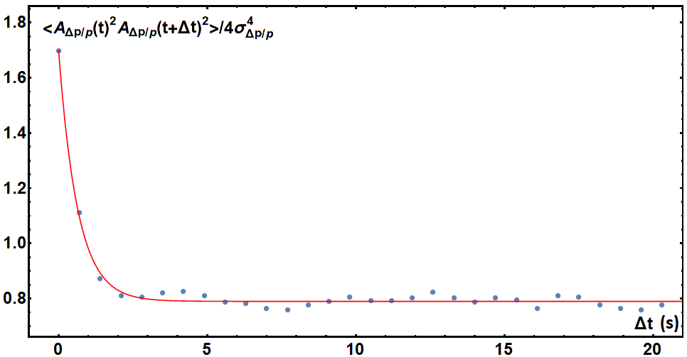
Figure 17 shows the autocorrelation of squared vertical amplitudes. For the empirical distribution of Eq. 5.2, all moments greater than the first are infinite. Therefore, mathematically, Eq. 4.8 is not applicable. In practice, in an experiment or simulation, all moments are finite due to limited observation time or finite aperture and the relation will hold. In the case of negligible background, the time constant of the exponential decay is unchanged. From this data set, we obtained the vertical amplitude damping time .


Another way to extract the vertical damping time is a direct analysis of the amplitude decays after large-amplitude scattering on the residual gas. The full data set contained 59 series that satisfied the following criteria:
-
•
was between 1.5 nm and 400 nm;
-
•
decreased compared to the previous measurement;
-
•
there were at least 5 points in the series.
Figure 18(a) shows all 59 selected series of amplitudes normalized to a 1 m beta function. The corresponding damping times, assuming zero vertical equilibrium emittance, are presented in Figure 18(b). The resulting vertical amplitude damping time is , which agrees with the results obtained from the autocorrelation analysis.
One can use the strong dependence of the vertical damping time on beam energy to estimate the energy of the electrons circulating in IOTA. Strongly suppressed transverse coupling makes the vertical damping time almost independent of the lattice configuration. For a flat ring with revolution period , the vertical damping rate is
| (5.3) |
with . The steep energy dependence gives favorable scaling for error propagation from damping time to energy. The two main systematic errors are transverse coupling and the actual magnetic field geometry of the main dipoles, which affects the integral of the squared curvature of the closed orbit. The latter effect was investigated using magnetic measurements and models of fringe fields of the main dipoles. Integration of 3D magnetic fields gives a 7.6% correction compared to the hard-edge model. For both types of main dipoles, a comparison between the measured and modeled fringe fields, accounting for known trims, yields a correction of less than 1% to the calculated energy value. To address the systematics due to coupling, we note that the horizontal damping time was longer than the vertical one. Therefore coupling between horizontal and vertical planes tends to increase the vertical damping time and therefore reduce the value of the beam energy. Experimental data showed that the vertical emittance contribution from coupling did not exceed 0.2 nm. If one introduces coupling randomly, so as to create a 0.2 nm increase in vertical emittance, the corresponding vertical damping time increases, on average, by 0.8%. The resulting IOTA beam energy estimate is .
5.4 Residual Gas Characteristics and Machine Aperture
Information about residual gas pressure and composition can be extracted from beam lifetime and from the statistics of small-angle scattering events in the vertical plane. Both processes are dominated by Coulomb scattering on residual gas nuclei. Other effects, such as bremsstrahlung and ionization losses, have significantly smaller cross sections.
The key difference between small amplitude scattering seen in the vertical plane and large amplitude kicks leading to particle loss is the impact parameter. The impact parameter determines the amount of nuclear screening by atomic electrons. Characteristic effects of nuclear screening and the relatively large number of small-angle impacts lead to a rough estimate of the gas composition. Anomalies in the gas composition may indicate leaks or other problems with the vacuum system. On the other hand, scattering to intermediate and large angles, when screening effects are small and the electron is lost, allow one to estimate the available aperture, which is helpful to understand the machine performance. Of course, the relatively low number of intermediate- and large-angle collisions results in large uncertainties on the aperture estimates.
The differential cross section for single Coulomb scattering with screening is given by the following approximate expression (see for instance Ref. [24], Section 3.3.1):
| (5.4) |
where .
For large dynamic apertures and relatively small threshold vertical angles , integration over all horizontal angles and integration over vertical angles exceeding gives the following cross section:
| (5.5) |
The frequency of excitations to an amplitude exceeding can be calculated as follows, taking into account the beta functions and partial pressures around the ring:
| (5.6) |
Here is the perimeter of the ring; is the effective gas density along the ring; are un-normalized relative gas densities. (Multiplying and dividing by allows one to use arbitrary nonzero coefficients as relative densities. For example, it is convenient to set one of the coefficients to 1.)


Experimentally, the dependence of the excitation frequencies on amplitude was extracted from the vertical amplitude time series, partially shown in Figure 10. First, the whole data array was filtered to exclude periods of a few very large excitations that made it impossible to detect small amplitude changes. Then, each amplitude jump was recorded. Special attention was given to properly treat transition frames, in which the electron oscillated with two significantly different amplitudes. Such frames typically result in a reconstructed amplitude that is in-between initial and excited values. A simplistic detection algorithm might count them as two events with smaller kicks. Instead, an interpolation method was used to get an estimate of the actual scattering amplitude.
Figure 19 shows the dependence of scattering frequencies on the effective vertical angle , assuming constant partial pressures around the IOTA ring. Figure 20 shows the same plot with normalized frequencies (i.e., frequencies multiplied by ). Without screening effects, the normalized frequencies should be independent of scattering amplitude. The small number of large-amplitude kicks results in noticeable discrete steps in the experimental data.
The plots show the experimental scattering frequencies together with 4 model curves for atomic numbers of 1 (hydrogen), 7 (nitrogen), 86 (radon) and for a combination of values 1 and 86. This combination, with partial coefficients and , showed the best fit, especially in the small-angle region, where most of the scattering events are concentrated. The resulting effective residual gas density is .
The ring aperture can be estimated from the large-amplitude scattering cross section, together with the known beam lifetime and effective residual gas density. For an elliptic aperture that requires kick angles much larger than for a particle to be lost, integration of Eq. 5.4 and averaging around the ring gives the following cross section:
| (5.7) |
The available data does not allow one to distinguish between restrictions in the vertical and the horizontal planes. The measured lifetime of 9100 s corresponds to apertures , assuming equal maximum amplitudes in both planes.
6 Conclusions
For the first time, to our knowledge, the dynamics of a single electron in a storage ring was tracked in all 3 dimensions using high-resolution synchrotron-light images acquired with digital cameras.
Data was taken at the Fermilab Integrable Optics Test Accelerator (IOTA) for both single electrons and for small countable numbers of electrons. A reliable and reproducible method to inject or remove a few electrons was developed. An absolute calibration of the camera intensity was implemented and its resolving power was evaluated. The beam lifetime at the lowest intensities was measured. In the central part of this work, we described how the horizontal, vertical and longitudinal oscillation amplitudes of a single electron were measured. From the time evolution of the oscillation amplitudes, several dynamical quantities were deduced, such as equilibrium emittances, momentum spread, damping times, and beam energy. The frequency distribution of residual-gas collisions events vs. scattering angle allowed us to estimate residual-gas pressure and composition and to give an approximate value for the machine aperture.
For the upcoming IOTA experimental runs, we plan to continue this research, adding to the camera images the synchronized acquisition of photon arrival times from the photomultipliers. This will allow us to record phase information for the betatron and synchrotron oscillations.
These measurements have a general scientific and pedagogic value, providing direct experimental insights into actual “single-particle dynamics” of an electron in a storage ring. In addition, these results provide information useful for machine commissioning, for beam instrumentation and diagnostics, and for verifying ring parameters obtained with more traditional techniques.
Acknowledgments
We would like to thank the entire FAST/IOTA team at Fermilab for making these experiments possible, in particular D. Broemmelsiek, K. Carlson, D. Crawford, N. Eddy, D. Edstrom, R. Espinoza, D. Franck, V. Lebedev, S. Nagaitsev, M. Obrycki, J. Ruan, and A. Warner.
This manuscript has been authored by Fermi Research Alliance, LLC under Contract No. DE-AC02-07CH11359 with the U.S. Department of Energy, Office of Science, Office of High Energy Physics. Work was supported in part by the U.S. National Science Foundation under award PHY-1549132 for the Center for Bright Beams and by the University of Chicago.
References
- [1] C. Bernardini, AdA: The first electron-positron collider, Physics in Perspective 6 (2004) 156.
- [2] L. Bonolis and G. Pancheri, Bruno Touschek and AdA: from Frascati to Orsay. in memory of Bruno Touschek, who passed away 40 years ago, on may 25th, 1978, Tech. Rep. 18-05/LNF, INFN, 2018.
- [3] F. Riehle, S. Bernstorff, R. Fröhling and F. P. Wolf, Determination of electron currents below 1 nA in the storage ring BESSY by measurement of the synchrotron radiation of single electrons, Nucl. Instrum. Methods Phys. Res. A 268 (1988) 262.
- [4] G. Brandt, J. Eden, R. Fliegauf, A. Gottwald, A. Hoehl, R. Klein et al., The Metrology Light Source — the new dedicated electron storage ring of PTB, Nucl. Instrum. Methods Phys. Res. B 258 (2007) 445.
- [5] R. Klein, R. Thornagel and G. Ulm, From single photons to milliwatt radiant power — electron storage rings as radiation sources with a high dynamic range, Metrologia 47 (2010) R33.
- [6] I. V. Pinayev, V. M. Popik, T. V. Shaftan, A. S. Sokolov, N. A. Vinokurov and P. V. Vorobyov, Experiments with undulator radiation of a single electron, Nucl. Instrum. Methods Phys. Res. A 341 (1994) 17.
- [7] A. N. Aleshaev, I. V. Pinayev, V. M. Popik, S. S. Serednyakov, T. V. Shaftan, A. S. Sokolov et al., A study of the influence of synchrotron radiation quantum fluctuations on the synchrotron oscillations of a single electron using undulator radiation, Nucl. Instrum. Methods Phys. Res. A 359 (1995) 80.
- [8] I. V. Pinayev, V. M. Popik, T. V. Salikova, T. V. Shaftan, A. S. Sokolov, N. A. Vinokurov et al., A study of the influence of the stochastic process on the synchrotron oscillations of a single electron circulated in the VEPP-3 storage ring, Nucl. Instrum. Methods Phys. Res. A 375 (1996) 71.
- [9] C. Koschitzki, A. Hoehl, R. Klein, R. Thornagel, J. Feikes, M. Hartrott et al., Highly sensitive beam size monitor for pA currents at the MLS electron storage ring, in Proceedings of the 1st International Particle Accelerator Conference (IPAC10), p. 894, IPAC’10 OC/ACFA, May, 2010, http://accelconf.web.cern.ch/IPAC10/papers/mopd084.pdf.
- [10] S. Antipov, D. Broemmelsiek, D. Bruhwiler, D. Edstrom, E. Harms, V. Lebedev et al., IOTA (Integrable Optics Test Accelerator): Facility and experimental beam physics program, JINST 12 (2017) T03002.
- [11] A. Romanov, D. R. Broemmelsiek, K. Carlson, D. J. Crawford, N. Eddy, D. R. Edstrom et al., Recent results and opportunities at the IOTA facility, Tech. Rep. FERMILAB-CONF-19-675-AD, Fermilab, 2020.
- [12] V. Danilov and S. Nagaitsev, Nonlinear accelerator lattices with one and two analytic invariants, Phys. Rev. ST Accel. Beams 13 (2010) 084002.
- [13] M. Church et al., Proposal for an accelerator R&D user facility at Fermilab’s Advanced Superconducting Test Accelerator (ASTA), Tech. Rep. FERMILAB-TM-2568, Fermilab, Oct., 2013. 10.2172/1422196.
- [14] A. Romanov et al., Commissioning and Operation of FAST Electron Linac at Fermilab, in Proceedings of the 9th International Particle Accelerator Conference (IPAC18), S. Koscielniak, T. Satogata, V. R. W. Schaa and J. Thomson, eds., (Geneva, Switzerland), pp. 4096–4099, JACoW, July, 2018, DOI [1811.04027].
- [15] A. Romanov, G. Kafka, S. Nagaitsev and A. Valishev, Lattice correction modeling for Fermilab IOTA ring, in Proceedings of the 5th International Particle Accelerator Conference (IPAC14), pp. 1165–1167, JACoW, June, 2014, DOI.
- [16] A. Valishev, N. Kuklev, A. Romanov, G. Stancari and S. Szustkowski, Nonlinear integrable optics (NIO) in IOTA Run 2, Tech. Rep. Beams-doc-8871, Fermilab, Nov., 2020.
- [17] S. A. Antipov, S. Nagaitsev and A. Valishev, Single-particle dynamics in a nonlinear accelerator lattice: Attaining a large tune spread with octupoles in IOTA, JINST 12 (2017) P04008.
- [18] N. Kuklev, Y.-K. Kim, S. Nagaitsev, A. Romanov and A. Valishev, Experimental demonstration of the Hénon-Heiles quasi-integrable system at IOTA, in Proceedings of the 10th International Particle Accelerator Conference (IPAC19), M. Boland, H. Tanaka and D. Button, eds., (Geneva, Switzerland), pp. 386–389, JACoW, May, 2019, DOI.
- [19] J. Safranek, Experimental determination of storage ring optics using orbit response measurements, Nucl. Instrum. Meth. A 388 (1997) 27.
- [20] V. Sajaev, V. Lebedev, V. Nagaslaev and A. Valishev, Fully coupled analysis of orbit response matrices at the FNAL Tevatron, Conf. Proc. C 0505161 (2005) 3662.
- [21] A. Romanov, D. Edstrom, F. A. Emanov, I. A. Koop, E. A. Perevedentsev, Y. A. Rogovsky et al., Correction of magnetic optics and beam trajectory using loco based algorithm with expanded experimental data sets, 1703.09757.
- [22] G. Stancari, A. Romanov, J. Ruan, J. Santucci, R. Thurman-Keup and A. Valishev, Notes on the design of experiments and beam diagnostics with synchrotron light detected by a gated photomultiplier for the Fermilab superconducting electron linac and for the Integrable Optics Test Accelerator (IOTA), Tech. Rep. FERMILAB-FN-1043-AD-APC, Fermilab, 2017.
- [23] G. Stancari, Beam lifetime from time intervals between single-electron losses in storage rings, Tech. Rep. FERMILAB-FN-1116-AD, Fermilab, 2020.
- [24] A. W. Chao, K. H. Mess, M. Tigner and F. Zimmermann, eds., Handbook of Accelerator Physics and Engineering. World Scientific, 2nd ed., 2013.