Exotic Image Formation in Strong Gravitational Lensing by Clusters of Galaxies – II: Uncertainties
Abstract
Due to the finite amount of observational data, the best-fit parameters corresponding to the reconstructed cluster mass have uncertainties. In turn, these uncertainties affect the inferences made from these mass models. Following our earlier work, we have studied the effect of such uncertainties on the singularity maps in simulated and actual galaxy clusters. The mass models for both simulated and real clusters have been constructed using grale. The final best-fit mass models created using grale give the simplest singularity maps and a lower limit on the number of point singularities that a lens has to offer. The simple nature of these singularity maps also puts a lower limit on the number of three image (tangential and radial) arcs that a cluster lens has. Hence, we estimate the number of galaxy sources giving rise to the three image arcs, which can be observed with the James Webb Space Telescope (JWST). We find that we expect to observe at least 20-30 tangential and 5-10 radial three-image arcs in the Hubble Frontier Fields cluster lenses with the JWST.
keywords:
gravitational lensing: strong – galaxies: clusters: individual (Abell 370, Abell 2744, Abell S1063, MACS J0416.1-2403, MACSJ0717.5+3745, MACS J1149.5+2223)1 Introduction
Galaxy clusters as strong lenses offer a unique probe to the matter distribution as lensing does not discriminate between the visible and dark matter distribution (e.g., Blandford & Narayan, 1992; Kneib & Natarajan, 2011). At the same time, by magnifying distant sources (which would have otherwise remained unobserved), it also opens up the possibility of studying the high-redshift Universe. Observation of these cluster lenses led us to the detection of multiply imaged supernovae (Kelly et al., 2015, 2016), which can help us in constraining the Hubble constant. On the other hand, the observation of highly magnified stars (Kelly et al., 2018) can help us in probing the mass-function of intra-cluster medium (Diego et al., 2018) and observing the pop III stars (Windhorst et al., 2018). Due to the high magnification provided by lensing, the detection of high-redshift () galaxies (e.g., Bradley, et al., 2008; Coe, et al., 2013; Watson, et al., 2015) can help in determination of the galaxy luminosity function (e.g., Atek et al., 2018).
In order to use galaxy clusters as a probe, we need to model their mass distributions. However, as the data from the observation is limited, one cannot model the mass distribution of these clusters with arbitrary precision and resolution. As a result, to reconstruct the lens mass distribution, different groups start with different sets of prior. For examples, light trace mass (LTM, Broadhurst et al., 2005; Zitrin et al., 2009) parametric mass reconstruction assumes that the mass distribution in the cluster lenses follows the light distribution. On the other hand, the non-parametric (free-form, Liesenborgs et al., 2007) mass reconstruction methods do not rely on any preliminary information related to the mass model and only take into account the strong and weak (Liesenborgs et al., 2020) lensing data. Hybrid mass reconstruction methods take input from both parametric and non-parametric approaches (Sendra et al., 2014). Due to the finite amount of data and different set of priors, it is possible that these different methods give different results when applied on the same cluster lens (e.g., Smith et al., 2009; Zitrin & Broadhurst, 2009). Hence, it is very important to compare these different techniques in case of simulated as well as real lenses to improve these methods and for more robust predictions (e.g., Meneghetti et al., 2017; Priewe et al., 2017; Rodney et al., 2015; Remolina González, Sharon, & Mahler, 2018; Raney et al., 2020). Each of these methods results into the best-fit mass model parameters and uncertainties associated with them. One avenue to observe the effect of these uncertainties is the cluster lens magnification maps. For the best-fit lens mass model, one will have a certain area in the lens plane that gives higher magnification than a threshold value. However, once we account for the statistical uncertainties, the area with a magnification greater than the threshold area is not a unique number; instead, it will be denoted by a range. As a result, various observational estimates (like the number of highly magnified galaxies) are also subjected to these uncertainties.
For a source to be highly magnified, the source must lie close to the caustic in the source plane and the corresponding images are formed near the corresponding critical line in the lens plane. The magnification factor by which the source is magnified also depends on the source size: smaller the source, larger the magnification factor, and vice versa. This is why one can have a magnification factor of thousands for lensed stellar sources (Kelly et al., 2018), whereas the maximum magnification factor for galaxy sources can only be in hundreds. These caustics and critical lines are the singularities of the lens mapping and are of two different types: stable and unstable. Fold and cusp are stable singularities as they are present for all source redshift, whereas beak-to-beak, umbilics, and swallowtails are unstable singularities as they only occur for specific source redshifts for a given lens system. So far, the number of known image formation near unstable singularities is very small: one near hyperbolic umbilic (Orban de Xivry & Marshall, 2009; Zitrin et al., 2010), handful near swallowtail (e.g., Abdelsalam, Saha, & Williams, 1998; Suyu & Halkola, 2010), and none near elliptic umbilic. With the upcoming observing facilities like: Euclid: (Laureijs, 2009), James Webb Space Telescope: (JWST, Gardner, et al., 2006), Nancy Grace Roman Space Telescope: (WFIRST, Akeson, et al., 2019), Vera Rubin Observatory: (LSST, Ivezić, et al., 2019), the number of strongly lensed system is expected to increase by more than an order of magnitude, and it is likely that we will encounter image formations near these unstable singularities. Hence, it is timely to explore the properties of these unstable singularities in detail.
In our previous work, we have described the method to locate these unstable singularities for a given lens model (Meena & Bagla, 2020, hereafter MB20) and applied this method in the case of actual cluster lenses (Meena & Bagla, 2021, hereafter MB21). The final output of this method is a singularity map containing all the point singularities and -lines. Since these -lines correspond to cusps in the source plane, they mark the high-magnification regions in the lens where image formation near cusps will occur (three or more lensed images lying near to each other). The point singularities depend on the second and higher-order derivatives of the lens potential. Hence, they are very sensitive to the presence of small/intermediate-scale structures and the variations in the lens parameters. As a result, the singularity maps corresponding to the parametric and non-parametric mass models can be very different for the same cluster lens As pointed out in MB21, parametric mass models give significantly larger number of point singularities due to the small scale structures compared to non-parametric mass models.
In our current work, we study the effect of the statistical uncertainties associated with the reconstructed lens mass model parameters on the singularity maps and the higher-order singularity cross-section. In order to study the effect of mass model uncertainties on the singularity maps, we have considered two simulated galaxy cluster lenses, Irtysh I and II from Ghosh, Williams, & Liesenborgs (2020, hereafter GWL20) and all of the six galaxy cluster lenses from the Hubble Frontier Fields (HFF) survey. The lens mass reconstruction of all of these cluster lenses has been done using grale111https://research.edm.uhasselt.be/jori/grale2/ (Liesenborgs et al., 2007). We choose the grale mass models as the corresponding singularity maps are simplest and provide a lower limit on the point singularity cross-section (MB21). Further, as the grale mass model does not make any assumption about density profiles of substructure, the reconstruction is independent of the nature of dark matter. Due to the simple nature, we can construct singularity maps for a larger region of the lens plane without introducing spurious point singularities. Apart from that, different grale runs for a cluster lens give independent mass maps. Hence, there is no correlation between different mass maps reconstructed for a lens using grale that may not be true for the parametric mass models. For simulated clusters, Irtysh I and II, we construct the singularity maps for the original mass models, for the individual runs (with 150, 500, 1000 lensed images) and for the final best-fit mass model. For HFF clusters, we construct the singularity maps for the individual runs and for the best-fit mass model obtained by the averaging of the individual runs.
As we know that the -lines in the singularity maps correspond to the cusps in the source plane. Hence, a singularity map also gives the information about the number of cusps formed in the source plane at a given source redshift. By drawing the critical lines for a given source redshift overlaid on the singularity map, one can calculate the number of cusps in the source plane by counting the points where a critical line and corresponding -line cut each other. As the grale best-fit mass models provide the simplest singularity maps, they also give the lower limit on the cusp cross-section. Hence, it is worthwhile to calculate the lower limit of the cusp cross-section in the HFF clusters using the grale best-fit mass models. Following that, we also estimate the (tangential and radial) arc cross-section in case of both simulated and HFF cluster lenses. The source galaxy luminosity function has been taken from Cowley et al. (2018, hereafter C18). In C18, authors estimate the number of galaxies expected in the deep galaxy surveys with the JWST in different the filters for different exposure time. Although the expected galaxy population in any of the JWST filter can be used in our study, we only considered the expected galaxy population in one JWST filter, F200W, with an exposure time of seconds (please see C18 for more details).
This paper is organized as follows. In §2, we briefly revisit the basics of the singularities in the strong lensing. In §3, we present our results for simulated Irtysh clusters. The corresponding singularity maps are discussed in §3.1, followed by the discussion of the redshift distribution of singularities in §3.2. The results for the HFF clusters are presented in §4. The corresponding singularity maps, redshift distribution of singularities, and the arc cross-section are discussed in §4.1, §4.2, and §4.3, respectively. Summary and conclusions are presented in §5. The cosmological parameters used in this work to calculate the various quantities are: .
2 Singularities in Strong Lensing


In this section, we briefly review the basics of singularities in strong gravitational lensing to set the notions and notations. For a more detailed discussion about singularities, we encourage the reader to see into MB20, and Schneider, Ehlers, & Falco (1992).
For a given strong lens system, magnification factor in the lens (image) plane is given as,
| (1) |
where and are the eigenvalues of the deformation tensor , with being the projected lens potential and subscript represents its partial derivatives with respect to the image plane coordinates. is the distance ratio, where and represent the angular diameter distance from the lens to the source and from the observer to the source, respectively. The points in the lens plane where are known as the singular points of the lens mapping (see MB20 for more details). The location of these singular points in the lens plane defines the critical curves and the corresponding points in the source plane are known as the caustics. The critical curves in the lens plane are smooth closed curves, and trace regions with high magnification, whereas their counterpart, caustic curves in the source are closed but not necessarily smooth. These caustics in the source plane are made of smooth segments (known as folds) meeting with each other at the cusp points.
For a given strong lens system, fold and cusp are the only stable singularity of the lens mapping as they are present for all possible source redshifts. The evolution of caustic structure in the source plane with source redshift mainly depicts the formation, destruction, or exchange of cusps between radial and tangential caustics. Other higher-order singularities (also known as point singularities) like swallowtail, purse, and pyramid are only present for specific source redshifts and are sensitive to the lens parameters. A small change in the lens system parameters can result in the complete disappearance of a point singularity. These point singularities, along with the -lines constitute the so called singularity map. -lines form the backbone of the singularity map and denote the points in the lens plane which correspond to the cusps in the source plane for all possible source redshifts. Different point singularities are associated with the formation, destruction, or exchange of cusp between radial and tangential caustics, hence, they also satisfy the -line condition along with additional criteria. -lines are given by the condition , where denotes the eigenvalue of the deformation tensor, and is the corresponding eigenvector. The swallowtail singularity denotes the points in the lens plane where the eigenvector is tangential to the corresponding -line, and at a swallowtail singularity two extra cusps appear in the source plane. The hyperbolic and elliptic umbilics mark the points in the lens plane where both eigenvalues of the deformation tensor are equal to each other, i.e., zero shear points. We encourage the reader to see MB20 for more details about the point singularities and the corresponding characteristic image formations.
As these point singularities depend on the second and high-order derivatives of the lens potential, the effect of variation of lens parameters can be seen clearly in the corresponding singularity map. As a result, the singularity map is also very sensitive to the lens mass reconstruction method, as shown in MB21. In MB21, one can see that the cluster mass models reconstructed using non-parametric method grale give a significantly lower number of point singularities compared to the parametric mass models for the same cluster, hence, putting the lower limit on the point singularity cross-section. The singularity maps corresponding to the non-parametric mass models also show very simple -line structures compared to the singularity map corresponding to the parametric mass models. Hence, the three image (tangential and radial) arc cross-section in parametric and non-parametric mass models is also expected to show significant differences.
3 Simulated Clusters


In MB21, it has been shown that the parametric and non-parametric mass models for a given HFF cluster show a significant difference in both cusp and point singularity cross-section. However, each mass model has uncertainties associated with it due to the finite amount of observational data. As a result, these uncertainties also affect the results derived from the reconstructed mass models. In this section, we study the effect of these uncertainties on the singularity maps corresponding to reconstructed mass models for simulated galaxy clusters. We have considered two simulated clusters, Irtysh I and II from GWL20. GWL20 reconstructed free-form mass models using grale for both Irtysh I and II with three different sets of multiple images, 150, 500, 1000. The lens mass reconstruction with 150 images corresponds to the current observational scenario, whereas the 500 and 1000 multiple image cases correspond to future observations with the Hubble Space Telescope (HST) and James Webb Space Telescope (JWST). For each case, individual mass models are obtained from forty different and independent grale runs and the final best-fit mass model is an average of the mass distributions from these forty independent grale runs. While constrained by the required computational resources this number is consistent with previous works with grale and it sufficiently spans the range of uncertainties in the reconstructed mass models. We refer the reader to look into GWL20 for more details. Hereafter, for simplicity, the average mass models for 1000, 500, 150 image cases for Irtysh I/II will be referred as Irtysh IA/IIA, IB/IIB, IC/IIC.
3.1 Simulated Clusters: Singularity Maps
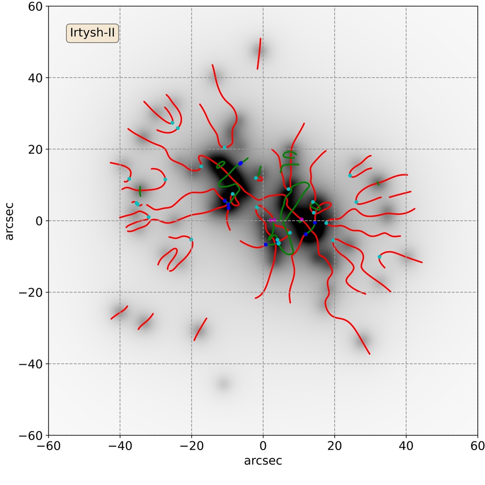
Once we have all the reconstructed mass models, we construct the singularity maps for all individual mass models and also for the final averaged one and the original mass models. To construct the singularity maps, we chose a resolution of in the lens plane to calculate relevant quantities. As discussed in MB21, for mass models reconstructed using grale, such a resolution of mass maps is adequate for constructing singularity maps. The singularity maps cover sources upto a redshift of ten. The singularity maps for the original and final averaged mass models for Irtysh I and II are shown in Figure 1 and 2, respectively. In each panel, the red and green lines represent the -lines corresponding to the and eigenvalues of the deformation tensor. The (hyperbolic and elliptic) umbilics are shown by the blue points, whereas the swallowtail singularities corresponding to and eigenvalues are denoted by cyan and magenta points, respectively. One example of singularity maps corresponding to individual runs for Irtysh IA/IB/IC, IIA/IIB/IIC are shown in Figure 9. For both Irtysh I and II, we see that final averaged mass maps are not able to recover the contribution of the marginally critical structures in the singularity maps. In a singularity map, such structures can be located by looking for the isolated -lines. Even if some of the individual runs are able to recover contribution from such marginal structures, it may be possible that these structures are not present in the final best-fit mass models due to the averaging over forty individual mass reconstruction. On the other hand, it is also possible to have some additional contribution from the spurious structures which are not present in the original mass distribution, as can be seen in Irtysh IIA in Figure 2.
Apart from that, one can also notice differences between the -line structures in the singularity maps near the core region of Irtysh clusters in the original and reconstructed mass models. These differences may be a result of the fact that in the reconstruction of Irtysh I and II, there are no sources below redshift one. This difference is more significant between the original and individual runs (Figure 9), but the averaging in the final best-fit mass model decreases this difference and brings the reconstructed mass distributions closer to the original ones.
3.2 Simulated Clusters: Redshift Distribution of Singularities
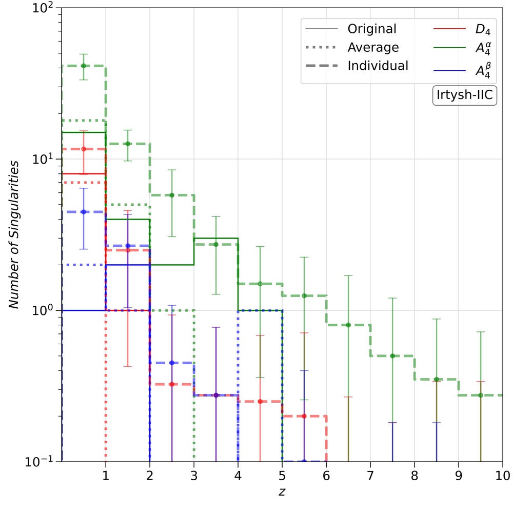
In this subsection, we study the redshift distribution of the point singularities for Irtysh I and II. In Figure 3, we represent the point singularities for different mass models as a function of redshift. Here we compare the number of singularities in the original Irtysh I and II mass models with the corresponding individual reconstructed mass models and with the corresponding final averaged mass model. For example, the top-left panel of Figure 3, shows the number of singularities in the original Irtysh I (thin lines), the number of singularities in the final averaged Irtysh IA mass model (thick dotted lines), and the average number of singularities in the corresponding individual runs (thick dashed lines). The error bars represent the one-sigma scatter within these forty individual runs. The red lines represent the (hyperbolic elliptic) umbilics. Here, we are not discriminating between hyperbolic and elliptic umbilics as the number of elliptic umbilics is very small compared to the hyperbolic umbilics. The green and blue lines represent the number of swallowtail singularities corresponding to and eigenvalues of the deformation tensor, respectively.
In each panel of Figure 3, for source redshift , we notice that the number of singularities in individual runs is significantly large compared to the number of singularities in the original mass Irtysh mass models, which is also evident from the individual runs in Figure 9. This is due to the fact that grale introduces a significant number of structure (which decrease as the number of lensed images increase) at different positions in each individual reconstruction, and as GWL20 do not have any sources at redshift , this effect is more significant in the central regions. As we move towards the higher source redshifts, the difference between original and individual run starts to narrow down. Although, the individual runs still predict slight excess of point singularities compared to the actual mass models.
Although the individual runs give a significant excess of point singularities below source redshift 2, such excess does not occur in the final averaged mass models. This behavior is expected from the fact that the averaging over multiple individual runs smooths out spurious structures and bring the final reconstructed mass model closer to the original mass model, although most of the time with slight underestimation of the point singularities. The averaging over multiple realizations sometimes also introduces a small number of spurious point singularities at high redshifts, for example, as seen in the Irtysh IA, Irtysh IIB, and Irtysh IIC panels in Figure 3. However, the number of these spurious singularities is not significant ( from Figure 3).
4 HFF Clusters
Under the Hubble Frontier Fields (HFF)
Survey222https://archive.stsci.edu/prepds/frontier/
program, Hubble Space Telescope observed a total of six
massive merging clusters (see Lotz et al. 2017
for more details).
For every HFF cluster, different groups have reconstructed mass
models using parametric, non-parametric and hybrid (a combination of
parametric and non-parametric) methods (e.g., Diego et al., 2007; Bradač et al., 2005; Jauzac et al., 2015; Johnson et al., 2014; Lam et al., 2014; Merten et al., 2011; Mohammed et al., 2016; Oguri, 2010; Sendra et al., 2014; Williams, Sebesta, & Liesenborgs, 2018; Zitrin et al., 2013).
To study the statistical uncertainties on the singularity maps, we
consider the non-parametric HFF cluster mass models.
These mass models for HFF clusters are reconstructed using the
free-form method grale.
There are two reasons for choosing these mass models for the HFF clusters:
(1) The best-fit grale mass models for HFF clusters gives the simplest
singularity maps compared to other techniques as shown in MB21 and
puts the lower limit on the point singularity cross-section.
Hence, it is worthwhile to check how statistical uncertainties affect
the lower limit.
(2) In MB21, we only considered the central region
for the analysis. This choice was made due to the increasing number of
spurious singularities in the parametric mass models as we go away from
the center of the cluster.
Hence, it will not be useful to analyze the effect of uncertainties on
the singularity map in the presence of artifacts.
However, such a problem does not exist for these non-parametric mass models
as the singularity map is very simple and a resolution of is
sufficient enough as shown in MB21.
Similar to the Irtysh clusters, for every HFF cluster, grale provides forty individual mass maps and one best-fit mass map that is the average of these forty mass maps. Depending on the number of images used in the reconstruction, there are different versions of the reconstructed mass models available. Here, we are using the v4 mass models for all of the HFF clusters, and, for simplicity, we will be using the abbreviated names for the HFF cluster lenses.
4.1 HFF Clusters: Singularity Maps
Following the procedure used for simulated clusters, we reconstruct the singularity maps for individual and the best-fit mass models of the HFF clusters. The best-fit mass model singularity maps for the HFF clusters are shown in Figure 4. Here again, the singularity maps are drawn for sources upto redshift ten. The red and green lines show the -lines corresponding to the and eigenvalues of the deformation tensor. The blue, cyan, and magenta points represent the (hyperbolic and elliptic) umbilics, swallowtail for , and swallowtail for eigenvalue, respectively. The online available v4 mass models have a resolution of . However, as the grale mass models are the superposition of a large number of projected Plummer density profiles, one can (in principle) resolve them up to any arbitrary resolution. In our current work, we use a resolution of for all of the HFF clusters. Although, as mentioned above, a resolution of is sufficient for grale mass models but, in order to be more certain that we did not miss any point singularities, we chose a resolution of (please see discussion about stability of point singularities in MB21).
We can see in Figure 4 that the A370 yields a very complex singularity map compared to other HFF clusters. Hence, the cross-section for image formation near a cusp or a point singularity is maximum for the A370 in the HFF clusters. One can also see that the point singularity cross-section calculation done in MB21 was based on the central region of ; however, the full singularity map extends upto a much bigger region in the lens plane for a source redshift of ten. Hence, the estimations done in MB21 are actually underestimates. Due to consideration of the central region, the cross-section of the hyperbolic umbilics was more than the swallowtails corresponding to the eigenvalues. However, looking at the complete singularity maps in Figure 4, one can see that the cross-section for the image formation near swallowtails corresponding to eigenvalue is higher compared to the hyperbolic umbilics as the outer regions of the singularity maps show more swallowtails than umbilics. This also explains why we observed a larger number of images near swallowtails (corresponding to eigenvalue) than hyperbolic umbilics. Here, we do not repeat that calculation and consider the earlier estimates as a lower limit.
Comparing the singularity maps of HFF clusters with each other one can also see that not all cluster lenses contribute equally in the point singularity or arc cross-section. For example, we can see that A370 is roughly five times more efficient in producing image formation near a swallowtail or a cusp compared to MACS0416. The efficiency of other HFF clusters lies between MACS0416 and A370. Such a difference is also observed in the corresponding magnification maps (e.g., Johnson et al., 2014; Vega-Ferrero, Diego, & Bernstein, 2019). However, one should keep in mind that the area in the source plane magnified by a factor has a significant contribution from the fold caustic. Hence, having a larger source plane area magnified by does not directly imply that the corresponding point singularity cross-section will also be higher. One can still use the magnification maps to get a qualitative idea about the arc and point singularity cross-section since large critical lines in the lens plane mean having more probability of a substructure introducing distortions in it and introducing extra cusps in the source plane. We would like to remind the reader that these inferences are based on specific models of HFF clusters, and these numbers can vary based on the reconstruction method used.
4.2 HFF Clusters: Redshift Distribution of Singularities
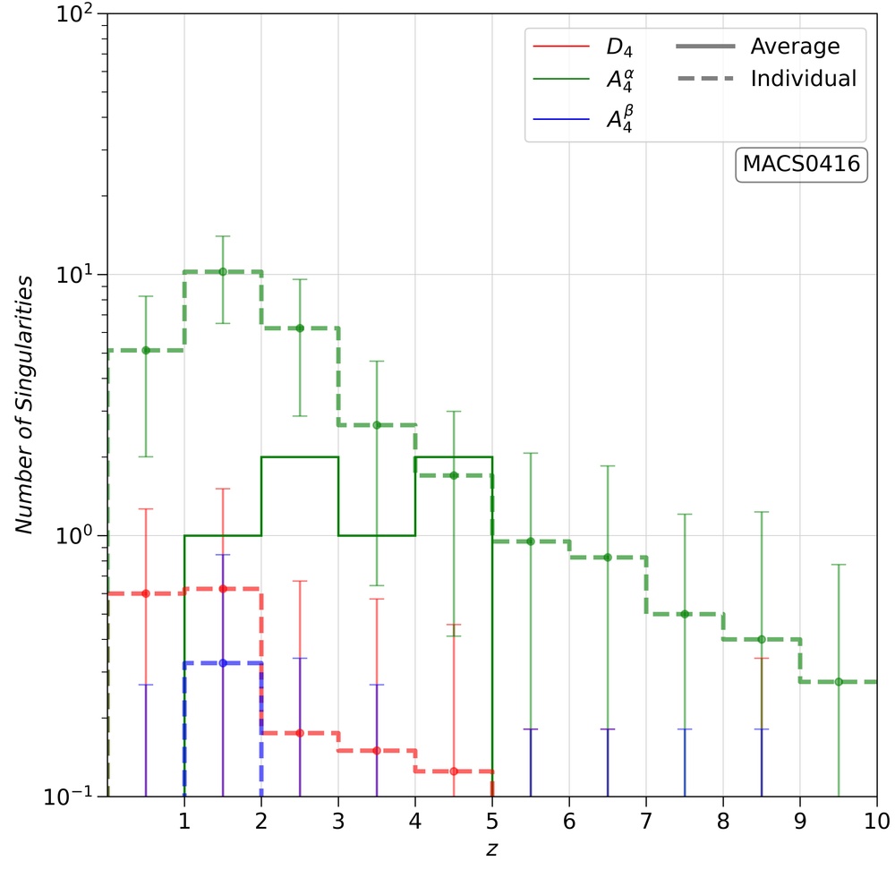
Unlike simulated clusters, we do not have the actual mass distribution of a real galaxy cluster. Hence, for HFF clusters, we compare the point singularities in the individual runs with the point singularities in the corresponding final best-fit mass models. The redshift distribution of point singularities in the HFF clusters is shown in Figure 6. In each panel, the red, green, and blue lines represent the number of (hyperbolic elliptic) umbilics, the number of swallowtail singularity for , and the number of swallowtail singularity for eigenvalues, respectively. Here, we do not differentiate between hyperbolic and elliptic umbilics as the number of elliptic umbilics is negligible as compared to the hyperbolic umbilics. In each panel, the thin solid lines represent the number of point singularities corresponding to the averaged best-fit mass models, and the thick dotted lines represent the average number of point singularities in the individual runs. The errorbars associated with thick dotted lines represent the one-sigma scatter in the number of point singularities in the 40 realizations.
As with the simulated Irtysh clusters, the average number of point singularities in the individual runs is higher (more than one sigma difference in some clusters) compared to the best-fit mass models at redshifts . In Irtysh clusters, we expected to observe such discrepancy in the central regions of the clusters as there were no sources below redshift one that can provide lensed images near the central region in order to constrain it better. For A370 and AS1063, there are lensed images below redshift one, but we still observe an excess of point singularities in the individual runs. Hence, we can say that introducing additional images below redshift one may help in decreasing the discrepancy in the central images. But we cannot be sure that it will always bring the numbers within one sigma error bars.
As we go towards higher source redshifts, the number of point singularities decreases in individual runs. However, the same cannot be said for the best-fit mass models. For example, in the case of A2744, there are some umbilics and swallowtails that are present even at very high source redshifts. Following the simulated Irtysh cluster, we may infer that these point singularities at very high redshift are spurious features. However, just by considering the grale mass models, we cannot be sure about that as there are no reference mass models for the real cluster lenses. As the point singularities depend on the higher-order derivatives of the deformation tensor, taking inputs from the parametric reconstruction for validations of these features may not be very useful.
4.3 HFF Clusters: Arc Cross-Section
The -lines constitute the backbone of a singularity map. These lines trace the points in the lens plane that correspond to cusps in the source plane. Hence, if we draw the critical curves for a given redshift on the top of the -lines in the lens plane then these critical curves cut the -lines at the points that correspond to cusps in the source plane for that source redshift. As a result, without looking into the source plane, one can count (in a very simple way) the number of cusps on tangential and radial caustics in the source plane. A source lying near a cusp in the source plane leads to the formation of a three-image arc. Hence, by using the -lines and the critical curves, we can easily calculate the three-image (tangential and radial) arc cross-section for a given lens model with a given population of sources.
To calculate the arc cross-section, we divided the source redshift range [0.6, 10] in equal intervals of . After that, we draw the critical curves in the lens plane for each interval and calculate the number of points in the lens plane where a (tangential or radial) critical curve cuts the corresponding -line. We assume that the number of such points is constant in the respective redshift interval of . Similar to point singularities in MB21, we consider an area of 5 kpc in the source plane and calculate the number of source galaxies with the image formation near the cusp points. This method will underestimate the number of cusp points if two -lines are very near to each other. Such a scenario occurs when a swallowtail singularity gets critical, and two cusps emerge in the source plane. However, the underestimation is not significant as the singularity maps for non-parametric models are not very complex.
Following this method, we calculated the cusp cross-section for HFF clusters. The galaxy source population is taken from C18 for one filter (F200W) of the JWST. The results are shown in Figure 7. The x-axis represents the source redshift, and the y-axis shows the number of source galaxies that are expected to give the image formation near cusps in the source plane higher than redshift . The red and green lines represent the number of source galaxies near the tangential and radial arcs in the source plane. In each panel, the cross-section is plotted considering sources in the redshift range [0.6, 10]. These cross-section plots again validate our inference from the singularity maps (in §4.1) that A370 is most efficient in producing the tangential and radial arcs among the HFF clusters. The cumulative arc cross-section for all clusters is shown in Figure 8. From our analysis, we expect to observe at least 10-20 tangential and 5-10 radial three image arcs with the JWST. Again, as the grale mass models have a very small contribution from galaxy scale substructures in the cluster lenses, these values should be considered as a lower limit. Since, grale provides a lower limit on the cusp cross-section, it will not be very beneficial to add the one-sigma error bars corresponding to individual runs in Figure 7 and 8. The reason is that the length of -lines in the individual runs is significantly larger than the averaged best-fit mass model and due to which these error bars will always be above the best fit lines.
5 Conclusions
In this work, we have studied the effect of statistical uncertainties associated with cluster lens mass reconstruction with grale on point singularities. We considered two simulated clusters, Irtysh I and II from GWL20 and six galaxy clusters from the HFF survey. For both simulated and real galaxy clusters, the mass models were reconstructed using grale. For each simulated galaxy cluster, we had three different mass models reconstructed with different sets of multiple images (please see GWL20 for more details). For each cluster lens, 40 reconstructions were done, and the best-fit mass models were the average of them. As a first step, we have constructed singularity maps for the original mass models (in the case of Irtysh I and II), for all of the individual mass models and for the best-fit mass models. In the next step, we have compared the singularity maps corresponding to the individual realizations with the original and average best-fit mass models. These comparisons for simulated and HFF clusters are shown in Figure 3 and 6, respectively.
We find that the singularity maps corresponding to the best-fit mass models have a relatively small number of point singularities compared to the individual runs. As a result, the best-fit mass models provide a lower bound on the number of singularities that a lens has to offer. For mass models reconstructed by grale, such a result is expected due to the fact that individual realizations contain spurious features, and the averaging to get the best-fit mass models is done in order to remove the contribution from these spurious features. Hence, the final best-fit mass model contains a low number of small scale structure and low number of point singularities. The differences in the number of point singularities between individual runs and the best-fit are maximum at source redshift for both simulated and real clusters. One can expect such discrepancy to arise at these redshifts as the mass models in the central regions of the clusters, at present, is not very well constrained. However, in order to be sure about this explanation, one will need to construct the mass models for simulated clusters with multiple images near the cluster center.
Such an averaging (over 40 realizations) to get the final best-fit mass model also simplifies the over -line structures in the singularity maps. As -lines in the singularity maps correspond to the number of cusps in the source plane at every source redshift, the final best-fit mass model also has a smaller number of cusps compared to individual realizations. Hence, the final best-fit mass models also provides a lower limit on the number of image formations near cusps. In our current work, we have also calculated the cusp cross-section for the HFF clusters using the best-fit mass models. we find that A370 is most efficient in producing three image arcs and the image formation near point singularities among the HFF clusters based on grale modeling. In the HFF clusters, one would expect to observe at least 10-20 tangential and 5-10 radial three image arcs with JWST.
The key take away from our current work is that the best-fit mass models constructed using the grale provide the lower limit on the number of cusps and point singularities for a given cluster lens. Folding in the statistical uncertainties does not decrease the numbers obtained from the best-fit mass models. As shown in MB21, one would expect to observe at least one hyperbolic umbilic and one swallowtail for every five clusters with JWST even when we include the corresponding statistical uncertainties. Apart from that, one also expects at least 10-20 tangential and 5-10 radial three image arcs with JWST in the HFF clusters.
The above results are based on the non-parametric modeling by grale, which underestimates the contribution from the galaxy scale substructures in the cluster lenses. Hence, if one considers parametric modeling, the above quoted numbers are expected to increase. As shown above, these singularity maps also provide a very nice way to compare the efficiency of different cluster lenses. This feature can also be used to compare the simulated and real clusters on qualitative (visual comparison of singularity maps) and quantitative basis (arc and point singularity cross-sections).
Apart from that, image formation corresponding to arcs or point singularities shows three or more images lie in a very small region of the lens plane. Hence, the time delay between these images is expected to be small compared to other (typical) multiple image formation scenarios. The other important feature of point singularities is their characteristic image formation, which can be very helpful in locating them. These possibilities are the subject of our ongoing work.
6 Acknowledgements
AKM would like to thank Council of Scientific Industrial Research (CSIR) for financial support through research fellowship No. 524007. Authors thank the anonymous referee for useful comments. This research has made use of NASA’s Astrophysics Data System Bibliographic Service. We acknowledge the HPC@IISERM, used for some of the computations presented here.
7 Data Availability
The simulated cluster (Irtysh I and II) data from GWL20 and the high resolution HFF cluster mass models corresponding to the Williams group are available from the modelers upon reasonable request.
References
- Abdelsalam, Saha, & Williams (1998) Abdelsalam H. M., Saha P., Williams L. L. R., 1998, MNRAS, 294, 734. doi:10.1046/j.1365-8711.1998.01356.x
- Akeson, et al. (2019) Akeson R., et al., 2019, arXiv, arXiv:1902.05569
- Atek et al. (2018) Atek H., Richard J., Kneib J.-P., Schaerer D., 2018, MNRAS, 479, 5184. doi:10.1093/mnras/sty1820
- Blandford & Narayan (1992) Blandford R. D., Narayan R., 1992, ARAA, 30, 311. doi:10.1146/annurev.astro.30.1.311
- Bradač et al. (2005) Bradač M., Schneider P., Lombardi M., Erben T., 2005, AA, 437, 39. doi:10.1051/0004-6361:20042233
- Broadhurst et al. (2005) Broadhurst T., Benítez N., Coe D., Sharon K., Zekser K., White R., Ford H., et al., 2005, ApJ, 621, 53. doi:10.1086/426494
- Bradley, et al. (2008) Bradley L. D., et al., 2008, ApJ, 678, 647
- Coe, et al. (2013) Coe D., et al., 2013, ApJ, 762, 32
- Cowley et al. (2018) Cowley W. I., Baugh C. M., Cole S., Frenk C. S., Lacey C. G., 2018, MNRAS, 474, 2352. doi:10.1093/mnras/stx2897
- Diego et al. (2007) Diego J. M., Tegmark M., Protopapas P., Sandvik H. B., 2007, MNRAS, 375, 958. doi:10.1111/j.1365-2966.2007.11380.x
- Diego et al. (2016) Diego J. M., Broadhurst T., Chen C., Lim J., Zitrin A., Chan B., Coe D., et al., 2016, MNRAS, 456, 356. doi:10.1093/mnras/stv2638
- Diego et al. (2018) Diego J. M., Kaiser N., Broadhurst T., Kelly P. L., Rodney S., Morishita T., Oguri M., et al., 2018, ApJ, 857, 25. doi:10.3847/1538-4357/aab617
- Gardner, et al. (2006) Gardner J. P., et al., 2006, SSRv, 123, 485
- Ghosh, Williams, & Liesenborgs (2020) Ghosh A., Williams L. L. R., Liesenborgs J., 2020, MNRAS, 494, 3998. doi:10.1093/mnras/staa962
- Ivezić, et al. (2019) Ivezić Ž., et al., 2019, ApJ, 873, 111
- Jauzac et al. (2015) Jauzac M., Richard J., Jullo E., Clément B., Limousin M., Kneib J.-P., Ebeling H., et al., 2015, MNRAS, 452, 1437. doi:10.1093/mnras/stv1402
- Johnson et al. (2014) Johnson T. L., Sharon K., Bayliss M. B., Gladders M. D., Coe D., Ebeling H., 2014, ApJ, 797, 48. doi:10.1088/0004-637X/797/1/48
- Kelly et al. (2015) Kelly P. L., Rodney S. A., Treu T., Foley R. J., Brammer G., Schmidt K. B., Zitrin A., et al., 2015, Sci, 347, 1123. doi:10.1126/science.aaa3350
- Kelly et al. (2016) Kelly P. L., Rodney S. A., Treu T., Strolger L.-G., Foley R. J., Jha S. W., Selsing J., et al., 2016, ApJL, 819, L8. doi:10.3847/2041-8205/819/1/L8
- Kelly et al. (2018) Kelly P. L., Diego J. M., Rodney S., Kaiser N., Broadhurst T., Zitrin A., Treu T., et al., 2018, NatAs, 2, 334. doi:10.1038/s41550-018-0430-3
- Kneib & Natarajan (2011) Kneib J.-P., Natarajan P., 2011, AARv, 19, 47. doi:10.1007/s00159-011-0047-3
- Laureijs (2009) Laureijs R., 2009, arXiv, arXiv:0912.0914
- Lam et al. (2014) Lam D., Broadhurst T., Diego J. M., Lim J., Coe D., Ford H. C., Zheng W., 2014, ApJ, 797, 98. doi:10.1088/0004-637X/797/2/98
- Liesenborgs et al. (2007) Liesenborgs J., de Rijcke S., Dejonghe H., Bekaert P., 2007, MNRAS, 380, 1729. doi:10.1111/j.1365-2966.2007.12236.x
- Liesenborgs et al. (2020) Liesenborgs J., Williams L. L. R., Wagner J., De Rijcke S., 2020, MNRAS, 494, 3253. doi:10.1093/mnras/staa842
- Lotz et al. (2017) Lotz J. M., Koekemoer A., Coe D., Grogin N., Capak P., Mack J., Anderson J., et al., 2017, ApJ, 837, 97. doi:10.3847/1538-4357/837/1/97
- Meena & Bagla (2020) Meena A. K., Bagla J. S., 2020, MNRAS, 492, 3294. doi:10.1093/mnras/stz3632
- Meena & Bagla (2021) Meena A. K., Bagla J. S., 2021, MNRAS, 503, 2097. doi:10.1093/mnras/stab577
- Meneghetti et al. (2017) Meneghetti M., Natarajan P., Coe D., Contini E., De Lucia G., Giocoli C., Acebron A., et al., 2017, MNRAS, 472, 3177. doi:10.1093/mnras/stx2064
- Merten et al. (2011) Merten J., Coe D., Dupke R., Massey R., Zitrin A., Cypriano E. S., Okabe N., et al., 2011, MNRAS, 417, 333. doi:10.1111/j.1365-2966.2011.19266.x
- Mohammed et al. (2016) Mohammed I., Saha P., Williams L. L. R., Liesenborgs J., Sebesta K., 2016, MNRAS, 459, 1698. doi:10.1093/mnras/stw727
- Oguri (2010) Oguri M., 2010, PASJ, 62, 1017. doi:10.1093/pasj/62.4.1017
- Orban de Xivry & Marshall (2009) Orban de Xivry G., Marshall P., 2009, MNRAS, 399, 2. doi:10.1111/j.1365-2966.2009.14925.x
- Priewe et al. (2017) Priewe J., Williams L. L. R., Liesenborgs J., Coe D., Rodney S. A., 2017, MNRAS, 465, 1030. doi:10.1093/mnras/stw2785
- Raney et al. (2020) Raney C. A., Keeton C. R., Brennan S., Fan H., 2020, MNRAS, 494, 4771. doi:10.1093/mnras/staa921
- Remolina González, Sharon, & Mahler (2018) Remolina González J. D., Sharon K., Mahler G., 2018, ApJ, 863, 60. doi:10.3847/1538-4357/aacf8e
- Rodney et al. (2015) Rodney S. A., Patel B., Scolnic D., Foley R. J., Molino A., Brammer G., Jauzac M., et al., 2015, ApJ, 811, 70. doi:10.1088/0004-637X/811/1/70
- Schneider, Ehlers, & Falco (1992) Schneider P., Ehlers J., Falco E. E., 1992, grle.book, 112. doi:10.1007/978-3-662-03758-4
- Sebesta et al. (2019) Sebesta K., Williams L. L. R., Liesenborgs J., Medezinski E., Okabe N., 2019, MNRAS, 488, 3251. doi:10.1093/mnras/stz1950
- Sendra et al. (2014) Sendra I., Diego J. M., Broadhurst T., Lazkoz R., 2014, MNRAS, 437, 2642. doi:10.1093/mnras/stt2076
- Smith et al. (2009) Smith G. P., Ebeling H., Limousin M., Kneib J.-P., Swinbank A. M., Ma C.-J., Jauzac M., et al., 2009, ApJL, 707, L163. doi:10.1088/0004-637X/707/2/L163
- Suyu & Halkola (2010) Suyu S. H., Halkola A., 2010, AA, 524, A94. doi:10.1051/0004-6361/201015481
- Vega-Ferrero, Diego, & Bernstein (2019) Vega-Ferrero J., Diego J. M., Bernstein G. M., 2019, MNRAS, 486, 5414. doi:10.1093/mnras/stz1217
- Windhorst et al. (2018) Windhorst R. A., Timmes F. X., Wyithe J. S. B., Alpaslan M., Andrews S. K., Coe D., Diego J. M., et al., 2018, ApJS, 234, 41. doi:10.3847/1538-4365/aaa760
- Watson, et al. (2015) Watson D., Christensen L., Knudsen K. K., Richard J., Gallazzi A., Michałowski M. J., 2015, Natur, 519, 327
- Williams, Sebesta, & Liesenborgs (2018) Williams L. L. R., Sebesta K., Liesenborgs J., 2018, MNRAS, 480, 3140. doi:10.1093/mnras/sty2088
- Zitrin & Broadhurst (2009) Zitrin A., Broadhurst T., 2009, ApJL, 703, L132. doi:10.1088/0004-637X/703/2/L132
- Zitrin et al. (2009) Zitrin A., Broadhurst T., Umetsu K., Coe D., Benítez N., Ascaso B., Bradley L., et al., 2009, MNRAS, 396, 1985. doi:10.1111/j.1365-2966.2009.14899.x
- Zitrin et al. (2010) Zitrin A., Broadhurst T., Umetsu K., Rephaeli Y., Medezinski E., Bradley L., Jiménez-Teja Y., et al., 2010, MNRAS, 408, 1916. doi:10.1111/j.1365-2966.2010.17258.x
- Zitrin et al. (2013) Zitrin A., Meneghetti M., Umetsu K., Broadhurst T., Bartelmann M., Bouwens R., Bradley L., et al., 2013, ApJL, 762, L30. doi:10.1088/2041-8205/762/2/L30
Appendix A Individual Runs
Figure 9, shows one individual run for each Irtysh IA, IB, IC, IIA, IIB, IIC. Similarly 10, Shows six individual runs for A370.


