Existence of The Closed Magnetic Field Lines Crossing The Coronal Hole Boundaries
Abstract
Coronal holes (CHs) are regions with unbalanced magnetic flux, and have been associated with open magnetic field (OMF) structures. However, it has been reported that some CHs do not intersect with OMF regions. To investigate the inconsistency, we apply a potential-field (PF) model to construct the magnetic fields of the coronal holes. As a comparison, we also use a thermodynamic magnetohydrodynamic (MHD) model to synthesize coronal images, and identify CHs from the synthetic images. The results from both the potential-field CHs and synthetic MHD CHs reveal that there is a significant percentage of closed field lines extending beyond the CH boundaries and more than 50% (17%) of PF (MHD) CHs do not contain OMF lines. The boundary-crossing field lines are more likely to be found in the lower latitudes during active times. While they tend to be located slightly closer than the non-boundary-crossing ones to the CH boundaries, nearly 40% (20%) of them in PF (MHD) CHs are not located in the boundary regions. The CHs without open field lines are often smaller and less unipolar than those with open field lines. The MHD model indicates higher temperature variations along the boundary-crossing field lines than the non-boundary crossing ones. The main difference between the results of the two models is that the dominant field lines in the PF and MHD CHs are closed and open field lines, respectively.
1 Introduction
Coronal holes (CHs) are observed as the darkest regions in the coronal images with predominantly unipolar magnetic fields at the photosphere. They are the regions with lower coronal emissions and density than the surrounding corona (e.g., Waldmeier, 1975; Zirker, 1977; Wiegelmann & Solanki, 2004) and an un-balanced magnetic-field distribution at the photosphere (e.g., Zirker, 1977; Cranmer, 2009; Hofmeister et al., 2017, 2019). The reconstruction of coronal magnetic fields from earlier studies indicate that CHs are often located in the regions with rapidly diverging “open” magnetic fields (e.g., Wilcox, 1968; Levine, 1982; Cranmer, 2009) which can accelerate plasma to supersonic outflows (Kopp & Holzer, 1976). “Open” magnetic fields (OMFs) are the magnetic structures that extend far away from the Sun. Therefore, CHs have been considered as major source regions for high-speed solar wind streams (Krieger et al., 1973, 1974).
However, more recent studies have shown significant inconsistency between the CHs and the source regions of high-speed solar wind (e.g., Huang et al., 2017), and between CHs and OMF regions (e.g., Obridko & Shelting, 1999; Lowder et al., 2014, 2017; Linker et al., 2017; Huang et al., 2017, 2019). Part of the inconsistency can be caused by methodological inaccuracy. For instance, different methods of extracting dark regions can result in 26% variation in the unbalanced flux (Linker et al., 2021). The choice of the boundary conditions in the model employed to construct the coronal magnetic fields can affect the topology of the determined OMF regions (Asvestari et al., 2019; Bertello et al., 2014; Caplan et al., 2021). In addition to the methodological uncertainties and inaccuracy, some physical effects/mechanisms are likely to also contribute to the inconsistency. For instance, Huang et al. (2019) show that OMF structures with higher super-radial expansion tend to be brighter. The analysis by Huang et al. (2019) reveals that some CHs (referred to as LIR in the paper) do not overlap with OMF regions, which indicates that these predominantly unipolar dark regions do not contain open magnetic field structures. While it has been known that closed-field structures exist inside the CHs (e.g., Wiegelmann & Solanki, 2004; Hofmeister et al., 2017, 2019; Heinemann et al., 2021b), these structures, being bi-polar, cannot contribute to the observed unipolarity of the region.
The objective of current study is to investigate the source for the absence of open magnetic structures in some CHs. The procedure is as follows: The first step is to construct synoptic maps of coronal images and magnetograms; second step is to identify the CHs from the maps based on a thresholding method; third step is to construct the coronal magnetic fields using Potential Field Source Surface (PFSS) model; fourth step is to compute the magnetic structures in the CHs by tracing the field lines from the surface up; and, lastly, different types of CH magnetic structures are identified and their characteristics examined. To investigate how the results would be affected by the current-free restriction in the PFSS model, we conduct a parallel examination using the synthetic coronal structures distributed by Predictive Science (Lionello et al., 2008), who computed the magnetic and thermal structures of the corona based on thermodynamic magnetohydrodynamics (MHD). We first construct a set of synthetic synoptic maps of coronal emission using the density and temperature in the MHD model, then identify synthetic CHs from the maps, and finally trace and examine the field lines in the synthetic CHs.
The observational data used for the study are described in Sec. 2. In Sec. 3, we explain the methods for constructing the synoptic maps (Sec. 3.1), identifying the coronal holes (Sec. 3.2), constructing the potential magnetic fields (Sec. 3.3), MHD modeling of the corona (Sec. 3.4) and the tracing of the field lines (Sec. 3.5). The results are presented in Sec. 4, discussed in Sec. 5, and summarized in Sec. 6.
2 Observational Data
The line-of-sight (LOS) magnetograms from Helioseismic and Magnetic Imager (HMI) and the 193 Å wavelength band images from Atmospheric Imaging Assembly (AIA), both onboard the Solar Dynamic Observatory (SDO), are used for the study. The time span of the data is from June 2010 to February 2020, corresponding to the Carrington Rotation (CR) number 2099 to 2227.
The monthly sunspot number (SSN) data distributed by Sunspot Index and Long-term Solar Observations, Royal Observatory of Belgium, Brussels (SILSO World Data Center), are used to evaluate the activity level of the Sun. To determine the SSN at a specific Carrington Rotation (CR), the monthly SSN is linearly interpolated to the time of the CR.
3 Method
3.1 Synoptic Map Construction
The LOS magnetic fields are converted into radial magnetic fields () assuming that the surface fields are radial (Svalgaard et al., 1978; Petrie & Patrikeeva, 2009; Gosain & Pevtsov, 2013). The synoptic maps of the radial fields and AIA 193 Å emissions are constructed using the stripes of around the central meridian. The size of the resulting maps is 3600 pixels in longitude () and 1440 pixels in sine-latitude ().
3.2 Coronal Hole Identification
The coronal holes are identified as the dark regions with predominantly unipolar magnetic field. The identification procedure consists of three steps: (1) extraction of dark regions from AIA 193Å synoptic maps; (2) evaluation of the stability of the dark-region boundaries, following the stability test procedure developed by Heinemann et al. (2019); and (3) evaluation of the level of unipolarity of the dark regions.
In the first step, an automated dark-region detecting procedure (Krista & Gallagher, 2009; Huang et al., 2019) is applied to AIA synoptic maps to determine an optimal intensity threshold of the Extreme UltraViolet (EUV) emission, , for each synoptic map. The determined of each synoptic map over the time period examined in this study is shown in Figure 1(a). The regions that are darker than and larger than 400 pixels ( Mm2) are extracted as dark regions.
In the second step, the stability of a dark region is evaluated by the variability of its area (area uncertainty) due to the variation of the intensity threshold (Heinemann et al., 2019). The smaller the area uncertainty, the higher the stability of the dark region. In brief, the stability evaluation is conducted as follows: The intensity threshold is varied from digital number (DN) to (DN), producing five area values (, to ) and an average area, , for each dark region. The area uncertainty of the dark region is subsequently computed as follows:
| (1) |
To determine the stability of the dark-region boundaries, we use a power function , where , and are the fitting parameters, to fit the scatter plot of vs. (shown in Fig. 1b). The best-fit curve is used as the bench mark to define high, medium and low stability regions: is high, is medium, and is low stability. They correspond to the green, yellow and red regions in Fig. 1b.
The third step is to determine the dark regions that are predominantly unipolar. A region with high level of unipolarity can be observed as a region with the radial-field distribution highly skewed toward one polarity, or with a large average radial field , or both. Since the radial fields are measured at the photosphere, the dark-region boundaries are projected down to the photosphere by assuming that the 193 Å images represent the corona at a height of 0.02 above the solar surface (Caplan et al., 2016; Huang et al., 2019). The histogram of the skewness of the dark regions is plotted in the upper left panel of Fig. 2. The x axis is , and y axis is the number of the dark regions. The vertical line marks the location of , which is approximately the turning point of the histogram. It is thus selected as the threshold for the skewness (Huang et al., 2019). To determine the threshold for , the percentage of the dark regions qualified as CHs is plotted as a function of threshold in the lower left panel of Fig. 2. In addition to the result of setting the skewness threshold (black line), the profiles of setting (blue) and 1.0 (red) are also plotted for comparison. The plot shows that the percentage of the dark regions qualified as CHs approaches a constant of after 3 Gauss. Therefore, 3 Gauss is chosen as the threshold, and the dark regions with Gauss or magnetic-field skewness are considered as predominantly unipolar, and identified as coronal holes.
Since the boundary of a dark region can be changed by the variation of the intensity threshold, and within the boundary can also be changed. We consider the dark regions that are qualified as coronal holes under all five intensity thresholds as reliable coronal holes. The regions that only satisfy the unipolarity criteria for some intensity thresholds are classified as uncertain coronal holes. The coronal holes identified from the synoptic maps of AIA 193Å and HMI radial fields are referred to as CH193 hereinafter.
3.3 PFSS Modelling
The global coronal magnetic field is often constructed by the Potential Field Source Surface (PFSS) model (Schatten et al., 1969), which is based on the assumptions that the current is zero in the region of interest and that the tangential magnetic field vanishes at the upper boundary, called “source surface”, leading to strictly radial field lines afterward. Earlier studies (e.g., Schatten et al., 1969) have shown that the current-free assumption is broadly valid in most part of the corona except for the regions with rapidly varying magnetic fields, such as sunspots and streamers.
In this study, the PFSS magnetic fields are computed using the Global Potential and Linear Force-Free Fields code (GLFFF; Jiang & Feng, 2012), which solves the Laplace equation by the relaxation method. The upper boundary, i.e., the source surface, is placed at from the Sun center (e.g., Wang & Sheeley, 1990; Obridko & Shelting, 1999). The upper boundary condition is that all field lines at the source surface are assumed to be radial. The lower boundary is at the solar surface, and the HMI magnetic field synoptic maps are used as the lower boundary condition. To comply with our computing capacity, the HMI synoptic maps (36001400 pixels) are down sampled by Sifting Convolution on the Sphere (Roddy & McEwen, 2021). In brief, we first apply a low-pass Gaussian filter on the spherical harmonic coefficients of the maps and then inverse transform them back to a size of 360 pixels in longitude () and 180 pixels in latitude (). The detail of the down sampling procedure is described in Appendix.
3.4 MHD Modelling
The data of MHD modelled solar corona for the time period studied in this work are from Predictive Science, who computed the magnetic and thermal structures of the corona using their Magnetohydrodynamic Algorithm outside a Sphere (MAS) code, which solves the full set of thermodynamic MHD equations. The plasmas are assumed to be collisional below and collisionless beyond . The energy equation in the code includes the contributions from coronal heating, dissipation and radiative loss.
Using the electron density and temperature in the MAS data, we compute the synthetic EUV emission maps at 193 Å wavelength by the following equation:
| (2) |
where are the electron number density and the electron temperature along the line of sight , and is the AIA-193 temperature response function. The coronal holes for the MHD model are identified following the same procedure described in Section 3.2: (1) the dark regions are extracted from the synthetic EUV synoptic maps by intensity thresholding, (2) their stability is evaluated by the stability test, and (3) a set of unipolarity criteria is applied to identify the coronal holes. The unipolarity criteria are determined by the same procedure described in Sec. 3.2: The histogram of is plotted in the upper right panel of Fig. 2. The vertical line in the upper right panel marks the location , which is where the slope of the histogram shows the sharpest change. The percentage of the qualified CHs as a function of is shown in the lower right panel of Fig. 2. The result of setting the skewness threshold to 0.2 is plotted in black, and compared with the results of setting the threshod to 0.1 (blue) and 0.5 (red). The plot shows that the percentage of the qualified CHs approaches a constant of after G. Therefore, G is selected as the threshold for . In short, based on these plots, we determine the unipolarity criteria for the synthetic maps to be or Gauss. The CHs identified from the synthetic synoptic maps will be referred to as synthetic MHD CHs or CHMHD, to be distinguished from CH193, the coronal holes identified from the AIA and HMI synoptic maps.
3.5 Field Line Tracing
The magnetic field lines are computed by tracing the field lines from the surface upward. The “open” magnetic field lines in a PFSS magnetic field are defined as the field lines reaching the source surface, which is from the Sun center. To define the OMF lines in the MHD magnetic fields, we computed the distance at which the thermal pressure of the MHD model becomes larger than the tangential magnetic pressure. The result indicates that except for CR2157, “open” MHD field lines can also be defined as the field lines reaching from the Sun center.
After the field line tracing, the field lines that are rooted in the reliable coronal holes are considered as reliable field lines to be used for the analysis of CH magnetic structures. Other field lines are categorized as uncertain field lines and discarded.
4 Results
4.1 Reliable coronal holes and field lines
The temporal variations of the optimal intensity thresholds in AIA-193 synoptic maps and in MHD synthetic EUV maps are plotted as black lines in Fig. 1a and b, respectively. The overplotted red lines are the SSN, and follow the y-axis on the right side. The panels show that the variations of both AIA and synthetic maps are large before 2016, when the solar activity is higher, and become small with approaching a constant after 2016, when the Sun becomes quieter.
The scatter plots of vs. are shown in Fig. 1b and d for the dark regions identified from the AIA-193 synoptic maps and synthetic EUV maps, respectively. The best-fit curves to the scatter plots are plotted as green dashed curves, and the functional forms printed in the titles of corresponding panels. The points corresponding to high, medium and low stabilities are located in green, yellow and red sections, respectively. Among the 3210 dark regions extracted from the AIA-193 synoptic maps, 1894 () regions are categorized as high stability, 1133 () as medium stability, and 183 () as low stability. From the synthetic EUV synoptic maps, 1506 dark regions are identified, of which 924 () are categorized as high stability, 308 () as medium stability, and 274 () as low stability.
The y-axis of the scatter plots show that the area uncertainties for AIA-193 dark regions are all less than 25% of their average areas while for the dark regions extracted from the synthetic EUV maps can be higher than 200%, indicating that the dark regions extracted from the AIA maps are more stable than those from the MHD synthetic maps. The large for the synthetic dark regions is because the synthetic EUV maps are smoother, i.e., the intensity gradient is smaller. As a result, a same change in from -2 to 2 DN results in larger area change.
Large area uncertainty can lower the reliability of the identified coronal holes. This is because the distribution of the magnetic field within the boundary is more likely to change from predominantly unipolar to non-unipolar, or vice versa, if the enclosed area is changed by a large percentage. Fig. 3 and Fig. 4 show such examples found in the AIA-193 synoptic map of CR2099 and synthetic EUV map of CR2100, respectively. The background images in Fig. 3a and Fig. 4a are the AIA-193 map and synthetic EUV map, respectively. The contours of different colors mark the boundaries of the dark regions determined by different intensity thresholds, as indicated next to the two panel (a). Both panels contain both high-stability dark region(s), of which the variation of intensity threshold leads to a relatively small area variation, and low-stability regions, of which the same threshold variation results in significant boundary changes.
By comparing the background images of Fig. 4a and Fig. 3a, we can see that the synthetic EUV map (Fig. 4a) is smoother than the AIA-193 map (Fig. 3a), and therefore the area uncertainty of the former is larger than that of the latter, as pointed out in the discussion of vs. scatter plots.
Fig. 3b and Fig. 4b show the coronal holes identified from the dark regions in Fig. 3a and Fig. 4a, respectively. The dark regions that do not qualify as coronal holes under any intensity threshold are not shown. The white and gray areas correspond to the reliable and uncertain coronal holes, and blue and red lines the reliable and uncertain field lines, respectively. The gray region indicated by the white arrow in each figure is an uncertain coronal hole whose average magnetic field and skewness are plotted as a function of intensity threshold in Panel (c). The dashed horizontal line in each Panel (c) marks the threshold of unipolarity ( G or for Fig. 3c, and G or for Fig. 4c). The and of the indicated gray regions are plotted as black and red lines, respectively. The x axis is the intensity threshold . follows the y axis on the left, and the y axis on the right.
Fig. 3c indicates that both and become lower than the unipolarity thresholds when is greater than approximately DN, disqualifying the region as a CH. Fig. 4c indicates that the indicated region in Fig. 4b is disqualified as a CH when is approximately 18 (17.5 DN DN), when both and are lower than the unipolarity thresholds. Since they are not qualified as coronal holes for all five intensity thresholds, these two regions are categorized as uncertain coronal holes. In contrast, the white regions in panel (b) of Fig. 3 and Fig. 4 satisfy the unipolarity criteria for all five intensity thresholds.
The field lines that are rooted in the reliable CHs are considered as reliable field lines. In total, 81.8% of the field lines in CH193 and 61.8% of the field lines in CHMHD are identified as reliable field lines. All CHs and field lines discussed in the rest of the paper are the reliable CHs and reliable field lines, and “reliable” will be dropped for brevity.
4.2 Boundary-crossing and non-boundary-crossing field lines
The examination of the field lines reveals that in addition to the well-known open magnetic field lines and closed field lines with both foot points located in the same CH, there are closed field lines that cross the boundary of the CH and end in either a bright region or a different CH. For conciseness, we use “1” and “0” to indicate the field-line foot points located inside and outside a CH, respectively, and abbreviate OPen and CLose as OP and CL. Therefore, OPen field lines will be referred to as OP1, and CLosed field lines with one foot point ending in a non-CH region will be referred to as CL10. To distinguish the CLosed field lines with both foot points rooted in a same CH and those connecting two different CHs, the former is referred to as normal CLosed field lines CL11n, and the latter as abnormal CLosed field lines CL11a.
The results of CR2105 are shown in Fig. 5 as an example. The field lines are computed from the PFSS magnetic fields. The background in all panels is the AIA 193 Å synoptic map projected to the solar surface, assuming that the height of the AIA 193 images is at . The white contours mark the identified CH193, and different types of field lines are plotted in different colors in separate panels, as indicated in the panel titles. Although OP1 (panel a) and CL10 (panel b) appear to be the dominant types for this Carrington Rotation, they occupy less than 21% and 28% of the total number of field lines in this Carrington Rotation, respectively. The most numerous type is actually CL11n (panel c). CL11n, while being shorter than the other three field line types, can be found in all CHs, and accounts for nearly 52% of the field lines in CR2105.
Comparing panel (a) and other panels, it can be seen that four CHs (indicated by white arrows) in this CR contain no OP1 and only closed field lines. CHs with such magnetic structures do not intersect with OMF regions, and would not be the source regions for high-speed solar wind streams. A close examination of panel (b) reveals that some brighter ends of CL10 are found in the neighborhoods of active regions and just outside the edges of another CH. CL11a, shown in panel (d), is usually the rarest among the four types. In this Carrington Rotation, they account for only 0.5% of the total number of the field lines. In this specific CR, they are seen to connect two CHs (marked in thicker contours) that are located in different hemispheres. Comparison with panel (b) shows that these two CHs are also connected by several CL10.
The field lines computed from the MHD model of the same Carrington Rotation, CR2105, are plotted in Figure 6 in the same format as Figure 5. The background in all panels is the synthetic EUV map and the white contours are the identified CHMHD. The synthetic map and CHMHD are qualitatively similar to, albeit spatially less resolved than, the observed AIA map and CH193 in Figure 5.
Figure 6 shows that the coronal holes from the MHD model contain all four types of the field lines: OP1 (panel a) is the most numerous field line type, accounting for of the total field lines in this CR, and CL11a (panel d) is the rarest type ( of the total number). Despite being the most numerous, OP1 does not exist in all CHMHD. In this Carrington Rotation, there are two CHMHD without any OP1, as indicated by the arrows. CL11n, which was the most numerous type in Figure 5, constitutes only of the total field lines in the CHMHD of CR2105, and does not exist in all CHMHD. Similar to the CL10 in the PFSS magnetic fields, the brighter ends of CL10 (panel b) in the MHD model are also found in the neighborhoods of active regions and near the boundary of another coronal hole.
4.3 Coronal holes without open magnetic field lines
As revealed in Sec. 4.2, there are coronal holes without open magnetic field lines. They constitute more than 50% of all CH193, and more than 17% of all CHMHD.
The CHs without OP1 are on average smaller than those with OP1. For CH193, the average area of the former is Mm2 and is Mm2 for the latter. For CHMHD, the values are Mm2 (without OP1) and Mm2 (with OP1).
To examine their magnetic fields, the histograms of and of the coronal holes with and without OP1 are plotted in Fig. 7, and the averages are printed in the corresponding panels. The upper four panels are the histograms of and the lower four the histograms of . The histograms for CH193 and CHMHD are placed in the left and right panels, respectively.
Compared with the histograms of the coronal holes with open magnetic field lines (panel a and e), the histograms of the CHs without OP1 (panel b and f) are more concentrated near lower with fewer cases at the high tail. This is especially prominent in panel f, with more than 50% of CHMHD concentrated at small ( G). The high average in panel f is caused by a few outliers with very large ( G). For the histograms of , the peaks of the distributions of the CHs with and without OP1 are at similar locations. However, the CHs without OP1 (panel d and h) have fewer cases than the CHs with OP1 (panel c and g) at the tails of high .
In short, these histograms indicate that, for both CH193 and CHMHD, the coronal holes without open magnetic field lines are less likely to have large and large skewness. In other words, CHs without OP1 are less unipolar than the CHs with OP1.
4.4 Comparison of different types of field lines
4.4.1 Distance to the boundary
The distance of a field-line foot point to the CH boundary is computed as the shortest arc distance (distance on a sphere) between the foot point and all boundary points of the CH. Small bright spots within the CH are filled before the computation. To compare the distance-to-the-boundary, , of different field lines in different CHs, we define normalized distance as , where is the maximum of all in a same CH. The cumulative probabilities of the normalized distances, , of different field-line types are plotted in Fig. 8. The x axis is , and y axis is the cumulative probability. The results of the PFSS magnetic fields and MHD magnetic fields are placed in the left and right columns, and different field-line types are shown in different rows, as noted in the panel titles.
The plots show that the initial slopes of the boundary-crossing field lines extending to a bright region (CL10) and to another coronal hole (CL11a) are slightly steeper than the slopes of the field lines confined in a same CH, indicating that the boundary-crossing field lines are located slightly closer to the boundaries than those confined in a CH. For instance, if we choose as the boundary region, the cumulative probabilities indicate that slightly more than 60% (80%) of CL10 and CL11a and slightly less than 60% (60%) of OP1 and CL11n in CH193 (CHMHD) are located in this boundary region. On the other hand, this also indicates that nearly 40% (20%) of the boundary-crossing field lines in CH193 (CHMHD) are not located in the boundary regions.
The dashed lines in the panels point to the normalized distances at which the cumulative probability reaches 0.9, which means 90% of field lines are within this normalized distance from the nearest boundary. For the PFSS magnetic field, 90% of OP1, CL10, CL11n and CL11a are located within 0.65, 0.59, 0.62 and 0.58 normalized distance from the CH boundary, respectively. For the MHD magnetic field, the distances are 0.68, 0.50, 0.69 and 0.43. The plot and these numbers indicate that, statistically, the boundary-crossing field lines, i.e., CL10 and CL11a, are located closer to the boundaries than the non-boundary-crossing ones are. The difference is larger in the MHD magnetic fields than in the PFSS magnetic fields.
4.4.2 Temperature distribution along the field lines
To investigate whether any heat imbalance may exist in the closed field lines connecting different regions, we use the electron temperature in the MAS data to calculate the ratio of the temperatures, , of the two foot points at 1.02 . For CL10, is defined as of the bright foot point and that of the dark foot point. For CL11a and CL11n, is the temperature of the lower-latitude foot point and that of the higher-latitude foot point. The histograms of are shown in Figure 9 along with the sketches of these field line types. The mean and Full Width at Half Maximum (FWHM) of each distribution are printed in respective panel. The distribution of CL10 shows that the mean is larger than 1. This indicates that, on average, the brighter foot point is hotter than the dark foot point. FWHM of the three panels shows that the distribution of CL11n is much narrower than that of CL10 and CL11a, indicating that the field lines connecting to different regions (i.e., CL10 and CL11a) are more likely to be non-isothermal than those confined in a same region (i.e., CL11n). This is consistent with the finding by Heinemann et al. (2021a), who reported that the temperature inside the coronal hole boundaries tends to be uniform. Although and may seem to indicate that the field lines connecting two different CHs are, on average, slightly more isothermal than those rooted in the same CHs, the difference is too small to be statistically significant.
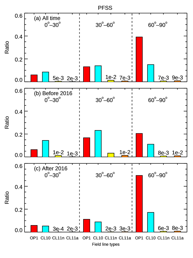
4.4.3 Dependence on latitude and solar activity
To examine whether the occurrence of different field-line types may be related to the latitudes and solar activity, we plot the ratio distributions of OP1, CL10, CL11a, and CL11n at different latitudes and different activity levels. The results from the PFSS (i.e., CH193) and MHD magnetic fields (i.e., CHMHD) are shown in Figure 10 and Figure 11, respectively. In each figure, different field-line type is represented by bars of different colors, as indicated. The heights of the bars correspond to the ratios relative to the total number of the lines in each panel. For the bars too short to be visible, the ratios are printed above the respective bars. The panels from top down show the ratio distributions of All time, Before 2016 (Active Time), and After 2016 (Quiet Time). In each panel, the distributions in low- (), mid- () and high- () latitudes are placed from left to right. For CL10 (the field lines extending to a non-CH region), the latitude is determined by the foot point in the coronal hole. For CL11a and CL11n (the field lines connecting different CHs and confined in a same CH), the latitude is determined by the foot point at the higher latitude.
One significant difference between the MHD and PFSS results is that the most numerous field line type is OP1 in CHMHD but is usually CL11n in CH193. Despite the differences, CL10 and CL11a, the two field line types that cross the boundaries of coronal holes, can be found in both PFSS and MHD magnetic fields, with higher occurrence during active time (panel b, before 2016). CL10 in the PFSS magnetic fields is the dominant type in the low-latitude () range, and is the second most numerous in the same latitude range in the MHD results. CL11a is more likely to be found in the low-latitude range in the MHD results and in the mid-latitude () range in the PFSS results. In both PFSS and MHD magnetic field, CL11a is the rarest type of field lines in the coronal holes. In short, Figure 10 and Figure 11 indicate that boundary-crossing field lines, CL10 and CL11a, are relatively more common when the Sun is more active.
5 Discussion
The lower ratio of CL11n in the MHD coronal holes can partly be due to the larger pixel size in the MHD data relative to that in the PFSS magnetic fields. Larger pixel size can significantly reduce the number of closed field lines inside the CHs because the bi-polar structures smaller than a pixel would not be resolvable. To test this proposition, we down-sampled the HMI synoptic maps to a spatial resolution of approximately 10∘, and re-calculated the ratio distributions of different field-line types. The result is plotted in Fig. 12. The format is same as that of Fig. 10. A comparison between Fig. 12 and Fig. 10 shows that the ratio of CL11n is significantly reduced after the down sampling. With the reduction of CL11n, OP1 becomes the most numerous field-line type in the high latitudes. In the mid- and low-latitudes, however, OP1 is still not as dominant over other field line types as seen in CHMHD (Fig. 11).
Another possible source for the dominance of OP1 in CHMHD is the the distance after which the field lines are considered open. In this study, this distance is chosen to be 2.5 from the Sun center. Although the thermal pressure is mostly higher than the tangential magnetic pressure in the MHD model at this distance, it is not impossible that some closed field lines can extend higher than this height. In the PFSS model, since the source surface is the upper boundary, changing its location can change the computed magnetic field, thereby changing the field lines. To check whether the relatively higher percentages of the boundary-crossing field lines and CHs without OP1 in the PFSS results may be reduced by changing the source surface distance, , we adjusted from 3.0 to 1.5 for six selected Carrington Rotations, three in the active times (CR2105, 2124, and 2136) and three in the quiet times (CR2174, 2179, and 2183). The results indicate that decreasing monotonically increases the ratio of OP1 and decreases that of the closed field lines, especially the boundary-crossing ones, thereby decreasing the percentage of CH193 without OP1. Nevertheless, there are still more than a quarter of CH193 without OP1 in these six selected Carrington Rotations even when is set at 1.5.
The differences in the approximations and assumptions implemented in the PFSS and MHD models inevitably also contribute to the difference in the percentage of OP1 between CHMHD and CH193, especially in the mid- and low-latitude regions. For instance, under the current-free restriction in the PFSS model, neighboring points with opposite polarities would be more likely connected by closed field lines, thereby lowering the number of OP1. The heating mechanisms implemented in the MHD model may lead to brighter foot points of closed field lines and darker OP1 foot points. As a result, the dark regions would consist of mostly open magnetic field lines.
In addition to the percentages of CL11n and OP1, the histogram of in the coronal holes without open magnetic fields (Fig. 7) and the cumulative probability of the distance to the boundary (Fig. 8) also reveal quantitative differences between the magnetic fields constructed in CHMHD and CH193.
In Fig. 7, panel f shows that of most CHMHD without OP1 is nearly zero. In other words, their is lower than the threshold of 2 G. Therefore, these regions can only be qualified as coronal holes due to skewed distribution of the magnetic fields. This indicates that while the percentage of the boundary-crossing field lines in these CHMHD is sufficiently high to skew the distribution of the signed magnetic field, their magnetic fields are not strong enough to shift the average .
In Fig. 8, all right panels (CHMHD) show a large cumulative probability at the zero normalized distance while the probability at the zeroth bin in the left panels (CH193) is very low. This is because the pixel size in the MHD maps and magnetic fields is much larger than that in the AIA-193 maps for the same CH area. Therefore, the chance of a pixel to be at the boundary is much higher in a CHMHD than in a CH193. Consequently, the probability for a field line to be in a boundary pixel is also higher in a CHMHD than CH193.
6 Summary
The coronal holes, being predominantly unipolar, are often considered to be the regions with open magnetic field lines and, therefore, source regions for high-speed solar wind. Huang et al. (2019), however, showed that some coronal holes do not intersect with open magnetic field regions, indicating that they do not contain open magnetic field lines. The aim of our study is to explain such inconsistency by examining the magnetic field structures of the coronal holes. We construct the magnetic fields in the coronal holes using PFSS model, and four types of magnetic structures are identified: open magnetic field line (OP1), closed magnetic field line confined in a same coronal hole (CL11n), closed field line with the other end extending to a bright region (CL10), and closed field line connecting two CHs (CL11a). As a comparison, we use the MHD model distributed by Predictive Science (Lionello et al., 2008) to compute synthetic coronal holes and their magnetic structures. All four types of magnetic structures are also found in the synthetic CHs. Despite some quantitative differences between the magnetic fields constructed by PFSS and MHD, the results from both models reveal that a significant number of coronal holes do not contain any open magnetic field lines and that their unipolarity is due to the closed field lines extending beyond the boundary of the coronal hole to a bright region (CL10) or another coronal hole (CL11a), with some CL10 connecting to an active region or ending near another coronal hole. Our results indicate that these CHs without OP1 are on average smaller and less unipolar than the CHs with open magnetic field lines. Such coronal holes are unlikely to be the source regions of high-speed solar winds, and can be one reason for the low consistency level between CHs and high-speed solar wind source regions reported by Huang et al. (2017).
The statistical analysis of the boundary-crossing field lines indicate that a non-negligible percentage of these field lines are not rooted in the boundary regions, and that they are more likely to occur during the active times. The temperature ratio of the field-line foot points indicates higher temperature variations along the boundary-crossing closed field lines than along the non-boundary-crossing ones.
These closed field lines connecting different coronal holes and between coronal holes and active regions may be formed by some prior dynamics and interactions between these regions, and may indicate some underlying large-scale magnetic structures connecting these regions, as suggested by Mogilevsky et al. (1997); Ioshpa et al. (1998). Investigation of these suppositions would require application of a time-dependent model to single magnetograms to better understand the formation mechanism and the physical properties of these field lines.
| (1) |
using the routine of SSWIDL, where is the radial component of magnetic field at colatitude and longitude , and is the complex conjugate of spherical harmonic function of degree and order , and is the harmonic coefficients of .
Next, a Gaussian function which peaks at and reduces to half maximum at is applied to :
| (2) |
where is the standard deviation of the Gaussian function.
Lastly, the low-pass filtered harmonic coefficients are transformed back to a coarser grid:
| (3) |
which contains 360 longitudes and 180 latitudes. Therefore, the smoothed HMI synoptic map has a size of . The inversion also uses the routine of SSWIDL.
References
- Asvestari et al. (2019) Asvestari, E., Heinemann, S. G., Temmer, M., et al. 2019, Journal of Geophysical Research (Space Physics), 124, 8280, doi: 10.1029/2019JA027173
- Bertello et al. (2014) Bertello, L., Pevtsov, A., Petrie, G. J. D., & Keys, D. 2014, Sol. Phys., 289, 2419, doi: 10.1007/s11207-014-0480-3
- Caplan et al. (2016) Caplan, R. M., Downs, C., & Linker, J. A. 2016, ApJ, 823, 53, doi: 10.3847/0004-637X/823/1/53
- Caplan et al. (2021) Caplan, R. M., Downs, C., Linker, J. A., & Mikic, Z. 2021, ApJ, 915, 44, doi: 10.3847/1538-4357/abfd2f
- Cranmer (2009) Cranmer, S. R. 2009, Living Reviews in Solar Physics, 6, 3, doi: 10.12942/lrsp-2009-3
- Gosain & Pevtsov (2013) Gosain, S., & Pevtsov, A. A. 2013, Sol. Phys., 283, 195, doi: 10.1007/s11207-012-0135-1
- Heinemann et al. (2021a) Heinemann, S. G., Saqri, J., Veronig, A. M., Hofmeister, S. J., & Temmer, M. 2021a, Sol. Phys., 296, 18, doi: 10.1007/s11207-020-01759-0
- Heinemann et al. (2019) Heinemann, S. G., Temmer, M., Heinemann, N., et al. 2019, Sol. Phys., 294, 144, doi: 10.1007/s11207-019-1539-y
- Heinemann et al. (2021b) Heinemann, S. G., Temmer, M., Hofmeister, S. J., et al. 2021b, Sol. Phys., 296, 141, doi: 10.1007/s11207-021-01889-z
- Hofmeister et al. (2019) Hofmeister, S. J., Utz, D., Heinemann, S. G., Veronig, A., & Temmer, M. 2019, A&A, 629, A22, doi: 10.1051/0004-6361/201935918
- Hofmeister et al. (2017) Hofmeister, S. J., Veronig, A., Reiss, M. A., et al. 2017, ApJ, 835, 268, doi: 10.3847/1538-4357/835/2/268
- Huang et al. (2017) Huang, G. H., Lin, C. H., & Lee, L. C. 2017, Scientific Reports, 7, 9488, doi: 10.1038/s41598-017-09862-2
- Huang et al. (2019) Huang, G.-H., Lin, C.-H., & Lee, L.-C. 2019, ApJ, 874, 45, doi: 10.3847/1538-4357/ab06f0
- Ioshpa et al. (1998) Ioshpa, B. A., Mogilevsky, E. I., & Obridko, V. N. 1998, in Astronomical Society of the Pacific Conference Series, Vol. 150, IAU Colloq. 167: New Perspectives on Solar Prominences, ed. D. F. Webb, B. Schmieder, & D. M. Rust, 393
- Jiang & Feng (2012) Jiang, C., & Feng, X. 2012, Sol. Phys., 281, 621, doi: 10.1007/s11207-012-0074-x
- Kopp & Holzer (1976) Kopp, R. A., & Holzer, T. E. 1976, Sol. Phys., 49, 43, doi: 10.1007/BF00221484
- Krieger et al. (1973) Krieger, A. S., Timothy, A. F., & Roelof, E. C. 1973, Sol. Phys., 29, 505, doi: 10.1007/BF00150828
- Krieger et al. (1974) Krieger, A. S., Vaiana, G. S., Timothy, A. F., Lazarus, A. J., & Sullivan, J. D. 1974, in Solar Wind Three, ed. C. T. Russell, 132–139
- Krista & Gallagher (2009) Krista, L. D., & Gallagher, P. T. 2009, Sol. Phys., 256, 87, doi: 10.1007/s11207-009-9357-2
- Levine (1982) Levine, R. H. 1982, Sol. Phys., 79, 203, doi: 10.1007/BF00146241
- Linker et al. (2017) Linker, J. A., Caplan, R. M., Downs, C., et al. 2017, ApJ, 848, 70, doi: 10.3847/1538-4357/aa8a70
- Linker et al. (2021) Linker, J. A., Heinemann, S. G., Temmer, M., et al. 2021, ApJ, 918, 21, doi: 10.3847/1538-4357/ac090a
- Lionello et al. (2008) Lionello, R., Linker, J. A., & Mikić, Z. 2008, ApJ, 690, 902, doi: 10.1088/0004-637X/690/1/902
- Lowder et al. (2017) Lowder, C., Qiu, J., & Leamon, R. 2017, Sol. Phys., 292, 18, doi: 10.1007/s11207-016-1041-8
- Lowder et al. (2014) Lowder, C., Qiu, J., Leamon, R., & Liu, Y. 2014, ApJ, 783, 142, doi: 10.1088/0004-637X/783/2/142
- Mogilevsky et al. (1997) Mogilevsky, E. I., Obridko, V. N., & Shilova, N. S. 1997, Sol. Phys., 176, 107, doi: 10.1023/A:1004908014970
- Obridko & Shelting (1999) Obridko, V. N., & Shelting, B. D. 1999, Sol. Phys., 187, 185, doi: 10.1023/A:1005188600022
- Petrie & Patrikeeva (2009) Petrie, G. J. D., & Patrikeeva, I. 2009, ApJ, 699, 871, doi: 10.1088/0004-637X/699/1/871
- Roddy & McEwen (2021) Roddy, P. J., & McEwen, J. D. 2021, IEEE Signal Processing Letters, 28, 304, doi: 10.1109/LSP.2021.3050961
- Schatten et al. (1969) Schatten, K. H., Wilcox, J. M., & Ness, N. F. 1969, Sol. Phys., 6, 442, doi: 10.1007/BF00146478
- Svalgaard et al. (1978) Svalgaard, L., Duvall, T., & Scherrer, P. 1978, Sol. Phys., 58, 225, doi: 10.1007/BF00157268
- Waldmeier (1975) Waldmeier, M. 1975, Sol. Phys., 40, 351, doi: 10.1007/BF00162382
- Wang & Sheeley (1990) Wang, Y.-M., & Sheeley, Jr., N. R. 1990, ApJ, 365, 372, doi: 10.1086/169492
- Wiegelmann & Solanki (2004) Wiegelmann, T., & Solanki, S. K. 2004, Sol. Phys., 225, 227, doi: 10.1007/s11207-004-3747-2
- Wilcox (1968) Wilcox, J. M. 1968, Space Sci. Rev., 8, 258, doi: 10.1007/BF00227565
- Zirker (1977) Zirker, J. B. 1977, Reviews of Geophysics and Space Physics, 15, 257, doi: 10.1029/RG015i003p00257