Existence of Non-singular Stellar Solutions within the context of Electromagnetic Field: A Comparison between Minimal and Non-minimal Gravity Models
Abstract
In this paper, we explore the existence of various non-singular
compact stellar solutions influenced by the Maxwell field within the
matter-geometry coupling based modified gravity. We start this
analysis by considering a static spherically symmetric spacetime
which is associated with the isotropic matter distribution. We then
determine the field equations corresponding to two specific
functions of this modified theory. Along with these models, we also
adopt different forms of the matter Lagrangian. We observe several
unknowns in these equations such as the metric potentials, charge
and fluid parameters. Thus, the embedding class-one condition and a
particular realistic equation of state is used to construct their
corresponding solutions. The former condition provides the metric
components possessing three constants, and we calculate them through
junction conditions. Further, four developed models are graphically
analyzed under different parametric values. Finally, we find all our
developed solutions well-agreeing with the physical requirements,
offering valuable insights for future explorations of
the stellar compositions in this theory.
Keywords: Electromagnetic field; Modified gravity; Junction
conditions; Stability.
I Introduction
Cosmologists have recently revealed revolutionary discoveries that defy traditional beliefs regarding the spatial organization of celestial structures in our cosmos. Rather than presenting a random dispersion, these formations exhibit a discernible order, sparking significant curiosity among researchers. The meticulous study of these entities has become a central topic of exploration for scientists committed to unraveling the mystery surrounding the accelerated expansion of the universe. Empirical testimonies strongly indicate the existence of an extensive counter-force to gravitational attraction, driving the observed rapid expansion. Referred to as dark energy, this enigmatic force presents a significant puzzle for scientists. While Einstein’s general relativity (GR) provides some insights into this expansion, it encounters difficulties in fully explaining dark energy, particularly in relation to the cosmological constant . Therefore, it has been necessary to introduce modifications to the existing theory to better comprehend and enhance our knowledge regarding fundamental dynamics of the cosmos.
Einstein’s GR has straightforwardly been modified to gravity, representing a substantial advancement in experimental physics. This theory alters the action function by interchanging the curvature scalar and its general functional. Notable progress has been made within this gravity theory, with implications reaching into the study of celestial structures 2 -4 . Astashenok with his collaborators 1n investigated the upper mass limit for massive objects in the current framework. Their research produced an intriguing result that as a second object in the binary GW190814, there must be either a rapidly rotating neutron star or a black hole. A significant body of literature underscores the remarkable contributions made by various researchers 1o -9 . One notable contribution comes from Bertolami and his colleagues 10 , who were instrumental in put forwarding the coupling between matter and spacetime geometry in gravity. Their methodology involved integrating the matter Lagrangian and into a unified functional form, known as theory. This novel concept prompted astronomers to focus on discussions related to the rapid universe’ expansion 11 .
Following these developments, Harko et al. 20 introduced a ground-breaking gravitational theory, called gravity at the action level. This theory utilizes a generalized function that leads to a non-conserved phenomenon, resulting in the emergence of an extra force, causing moving particles to follow non-geodesic path 22 . Houndjo 22a employed a particular model based on the minimal interaction to explain the shift from one cosmic era to the other phase in which we are living right now. Among the various functional forms of theory, the candidate has attracted considerable attention in scientific literature due to its ability to generate physically existing internal structures. Different researchers, including Das et al. 22b , utilized a similar model to develop a three-layer gravastar geometry. Various methodologies were implemented to explore diverse geometrical structures in this context 25af -25ae . An essential facet of the gravity is its incorporation of some effects at quantum level, which introduces the potential for particle creation. This characteristic is of great significance in astronomical investigations as it sets out a connection between the extended theory and quantum mechanics. Notable findings in this area have been produced and can be seen in 1j ; 1k . In a recent research endeavor, Zaregonbadi et al. 1l have examined the feasibility of this modification to GR to study the impact of dark matter on clusters of galaxies.
The theory has indeed presented an intriguing extension to GR, showing a diverse range of phenomenology in modern research. However, researchers 25ag ; 25aga delved into the challenges associated with constructing a viable and realistic cosmology within this theory. Their study demonstrated that the currently discussed models of this theory do not yield an expandable cosmic background. In response to these challenges, Haghani and Harko 25ah undertook a considerable effort by simultaneously unify two categories of gravitational theories, and call it the gravity. This strategic approach aims to address the limitations encountered in the previously discussed gravity models and offers a more comprehensive understanding of the intricate dynamics governing the universe. They explored the Newtonian limit of the field equations and provided some terms representing an extra-acceleration, particularly focusing on scenarios involving small velocities of particles and weak fields of gravity. This exploration enlightens how different choices of Lagrangian influence the description of the cosmic expansion. Zubair et al. 25ai reconstructed some cosmological solutions such as de Sitter and CDM models in this theory and found them to be cosmologically stable through suitable perturbations.
The study of celestial entities characterized by the field equations possessing high non-linearity, either in the framework of GR or extended theories, has prompted astronomers to actively seek their numerical or exact solutions. The significance of compact interiors lies in the physical interest they hold, contingent upon the satisfaction of specific conditions by the developed model. Various methodologies have been engaged in the scientific literature to derive such solutions, including the utilization of a specific ansatz or the implementation of particular equations of state, among other techniques. One approach to solving this challenge is through the implementation of the embedding class-one phenomenon, which posits that one can embed any space in another having at least one higher dimension. Bhar et al. 36 employed the same method, coupled with particular metric potentials and derived physically existing anisotropic solutions. Maurya et al. 37 ; 37a used the same approach to construct a new solution, delving into its stability and exploring the impact of anisotropic pressure on relativistic systems. Singh with his collaborators 37b devised a singularity-free solution for spherical geometry by proposing a specific metric function within the framework of this technique. Exploring this condition into a matter-geometry coupled theory, several works have yielded stable as well as viable solutions 38c -38a .
In this paper, we explore various isotropic solutions in conjunction with the Maxwell field within the framework of theory. The paper’s structure is organized as follows. The following section establishes some basics of this extended theory and derives the generalized field equations. Section III presents the Karmarkar condition, which aids in determining the metric potentials. Additionally, we utilize the Reissner-Nordström vacuum solution and compute the constants associated with the overhead condition. We outline particular criteria that, once fulfilled, guarantee the model’s physical validity in section IV. Advancing further, section V reveals the newly formulated solutions and offers a visual representation to aid in understanding the physical relevance of the obtained results. Conclusively, in the final section, our findings are encapsulated, summarizing the main outcomes and insights acquired in this study.
II Fundamentals of Modified Theory
The action of the modified theory is obtained after replacing the Ricci scalar with this functional 25ah . This has the form
| (1) |
where the electric charge and ordinary matter have Lagrangian densities, denoted by and , respectively. Also, with being the metric tensor and the two lines enclosing it symbolize the determinant. Varying the action (1) w.r.t. , the tensorial form of the modified field equations become
| (2) |
where the entity , namely the Einstein tensor, expresses the geometry of the considered fluid distribution and refers to the matter enclosed by that geometry. This effective term is further classified into three different energy-momentum tensors as
| (3) |
where
-
•
correspond to the ordinary matter configuration,
-
•
indicates the presence of charge in the self-gravitating system,
-
•
are modified correction terms.
We express as follows
On the other hand, the last term on the right side of Eq.(3) have the value given by
| (4) |
where , and . The mathematical definitions of the D’Alembertian operator and covariant derivative are and , respectively. Equations (2)-(4) provides after combining as
| (5) |
The energy-momentum tensor plays a pivotal role in formulating the gravitational field equations, enabling a precise representation of the interaction between matter and spacetime curvature. This tensor proves indispensable in understanding a wide array of physical phenomena, from celestial bodies’ gravitational influences to the dynamics of fluid systems. Its incorporation not only facilitates the development of accurate models for diverse astrophysical scenarios but also contributes to the exploration of fundamental principles in the broader context. The models possessing the isotropic fluid among all existing in the literature holds significance. Its application proves instrumental in various scientific disciplines, contributing to the development of accurate and tractable models for the study of diverse physical processes. Such matter distributions can be defined in the following way 1i
| (6) |
where being the pressure, symbolizes the energy density and indicates the four-velocity. The stress-energy tensor expressing the electromagnetic field is defined by 38b
whereas we can write Maxwell equations in concise (or tensorial) form as
| (7) |
Here, is written in terms of the four potential defined by . Also, the current and charge density are combined with each other through the relation .
Determining the trace of Eq.(5), we have the following
As functional of this theory is generalized in terms of the geometry and matter terms, the divergence of the stress-energy tensor becomes non-null. As a result, a supplementary force emerges within the gravitational field of a massive object, leading to modifications in the geodesic trajectory of moving test particles. This force is mathematically expressed as follows
| (8) |
Considering a spherical spacetime as an interior geometry is a significant starting point as its investigation involves understanding the curvature dynamics and gravitational interactions specific to a spherical space. The following metric represents such geometry as
| (9) |
where radial/temporal components depend only on the radial coordinate, showing that the geometry under consideration is static. We observe the presence of the four-vector in Eq.(6) which now becomes
| (10) |
Equation (7) (left) along with the metric (9) yields
where . Implementing an integration on the above second-order equation results in the following expression
where the total interior charge is defined as .
The isotropic modified field equations representing spherical structure are now formulated by combining Eqs.(5), (6) and (9). The non-vanishing components are given by
| (11) | ||||
| (12) | ||||
| (13) |
Also, the terms and are defined as
Solving Eqs.(11)-(13) presents a complex challenge due to the intricate relationships among multiple quantities, including . To address this complexity and arrive at a definitive solution, it is essential to introduce specific constraints. Without these constraints, obtaining a unique solution proves to be an insurmountable task.
II.1 Embedding Class-one Condition and Smooth Matching of Interior and Exterior Spacetimes
The incorporation of embedding class-one condition is crucial in discussing compact stars as they provide essential constraints and insights into the equilibrium and stability of these astrophysical objects. This mathematical condition contribute to a more comprehensive understanding of the physical properties governing celestial systems, aiding researchers in formulating accurate models and predictions for their behavior in extreme environments. According to this, if a tensor possessing the property of being symmetry fulfills the Gauss-Codazzi equations given in the following
| (14) |
then an -dimensional space can be embedded into the space of -dimension. Here, and symbolize the coefficients of second differential form and the curvature tensor, respectively, and . The above left equation, known as the Gauss equation, characterizes the intrinsic geometry of the surface by relating its curvature to that of the ambient space. This equation is crucial for understanding how the surface curves within the space it is embedded. On the other hand, the Codazzi-Mainardi (or Codazzi) equation given on the right side, expresses the compatibility between the intrinsic and extrinsic geometry of the surface. Mathematically, this condition can be written as follows 41i
| (15) |
resulting in the second-order differential equation after merging with the metric (9) as
| (16) |
that provides one component, say radial, in terms of the temporal coefficient. This takes the form
| (17) |
involving as an integration constant. To calculate the component accurately, it is essential to adopt the temporal coefficient. For this, we refer to widely recognized component within the astrophysics research community 37 ; 37a . This is taken by
| (18) |
possessing two positive constants, denoted as and , the values of which remain unspecified yet. Lake 41j introduced a criterion to assess the physical relevance of the metric potentials under consideration. By applying this evaluation to the specific component (18), it is determined whether such component holds significance in the context of the study. Therefore, we have
We notice that and at , representing the star’s center. This validates the suitability of Eq.(18). Upon insertion into Eq.(17), the function assumes the following value
| (19) |
where .
By enforcing consistency at the boundary of the object, junction conditions enable a smooth transition between different regions of spacetime, preserving the physical integrity of the model. This is crucial for accurately representing the gravitational field both inside and outside the compact object, contributing to a more realistic understanding of its structure and gravitational effects. Since a charged interior sphere (9) is considered, it must be adopted the Reissner-Nordström metric as an exterior spacetime. With and as the total charge and mass, this metric is given as follows
| (20) |
It must be stressed here that the first fundamental forms equals the radial as well as temporal components of both of the exterior and interior spacetime at the surface boundary, say mathematically . This is also true for the term . Following this, we have
| (21) | |||||
| (22) | |||||
| (23) |
The quartet () can now be easily found by simultaneously solving Eqs.(21)-(23). Their values are
| (24) | |||||
| (25) | |||||
| (26) | |||||
| (27) |
Determining the dimension of these constants is significant in such analysis of the compact stars. We find that the constant has a dimension of and having . However, the other constants, i.e., and have null dimensions. The graphical interpretation of the solutions (which shall be obtained later) needs some definite values of these constants. In order to make this possible, a star LMC X-4 is considered along with its observed data 42aa . In the following, the numerical values of these four constants are calculated in Tables I and II for multiple stars by choosing the exterior charge as and , respectively with being the mass of the Sun.
| Compact Stars | LMC X-4 | 4U 1820-30 | SMC X-4 | SAX J 1808.4-3658 | Her X-I |
|---|---|---|---|---|---|
| 1.04 | 1.58 | 1.29 | 0.9 | 0.85 | |
| 9.1 | 7.95 | 8.1 | 8.831 | 8.301 | |
| 187.321 | 162.134 | 181.623 | 190.332 | 213.199 | |
| 0.00211845 | 0.00316083 | 0.00241950 | 0.00197398 | 0.00170023 | |
| 0.471224 | 0.289282 | 0.390542 | 0.519452 | 0.552855 | |
| 2.99193 | 2.37202 | 2.74590 | 3.12262 | 3.20645 |
| Compact Stars | LMC X-4 | 4U 1820-30 | SMC X-4 | SAX J 1808.4-3658 | Her X-I |
|---|---|---|---|---|---|
| 201.499 | 169.301 | 191.865 | 207.971 | 233.803 | |
| 0.00199084 | 0.00302633 | 0.00230181 | 0.00183519 | 0.00157849 | |
| 0.486203 | 0.300188 | 0.40315 | 0.536174 | 0.569192 | |
| 3.12067 | 2.46086 | 2.84874 | 3.27424 | 3.36101 |
The relation between the values of and the electric charge is evident, as an increase in the later term is directly associated with the variations in these three constants. However, the value of is decreased as the electric charge is increased.
III Physical Requirements admitting by Stellar Models
In this section, we review multiple conditions that have been discussed in the literature whose satisfaction leads to the compact interior models to be physically relevant ab -af . We highlight some interesting and necessary conditions among them that must be discussed while studying the stars in the following.
-
•
A critical aspect involves the investigation of geometric quantities such as and . It must be verified that both these components are positive to maintain physical significance. Additionally, the regularity of these functions should be confirmed within the defined physical domain, ensuring they do not exhibit singularities.
-
•
Within compact stars, the behavior of energy density and pressure, along with their first two derivatives, is critical in understanding the internal configuration of these astrophysical objects. Typically, as one moves from the stellar surface towards the center, both these parameters tend to increase, reaching their maximum values at the core. The first derivatives with respect to radial distance capture the rate of change of these quantities, highlighting the distribution of mass and the response of matter to gravitational forces.
-
•
A point of discussion among researchers is the mass function that describes the fluid content enclosed by a body. This helps in understanding the gravitational impact of that structure. We express this in the form of energy density as
(28) The strength of a field surrounding a self-gravitating structure due to its gravity in relation with its size is measured by the compactness. It is actually a ratio between the mass of a body and its radius. Its expression is given by
(29) which must be less than to get a physically relevant interior 42a . The redshift characterizes the extent to which photons are stretched as they climb out of the gravitational well of a compact star. We describe it as
(30) It has been found that the redshift at the surface boundary must not be higher than 42a , i.e., . On the other hand, when Ivanov dealt with anisotropic pressure fluid, he established this limit to be 42c .
-
•
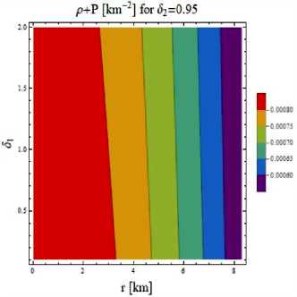
The incorporation of energy conditions holds paramount significance in discussions about compact stars. These conditions play a pivotal role in constraining the matter distribution within these dense astrophysical objects. By imposing constraints on energy density and pressure, energy conditions ensure the physical viability of solutions, guiding the development of realistic models for self-gravitating structures. Upholding these conditions not only fosters mathematical consistency but also provides crucial insights into the nature of matter supporting these stellar objects. For the case of charged fluid, they have the form
-
•
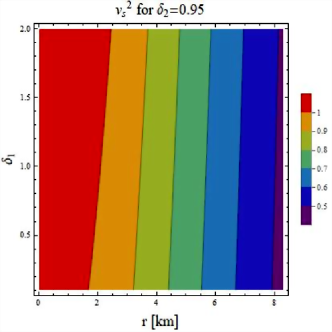
Various approaches have been proposed to assess the stability of celestial systems, with one method involving the consideration of the causality condition derived from the sound speed, expressed as . According to Abreu et al. 42bb , this condition ensures that information within the stellar medium propagates at speeds less than the speed of light, preventing causality violations, i.e., . At the same time, one can check the stability by studying the thermodynamic behavior of the celestial object. This can be discussed through the adiabatic index, indicated by , whose formula is given as follows
To maintain the equilibrium of a compact model, the outward pressure must be as enough as it can counterbalance the force of gravity acting inward. This can only be achieved if the adiabatic index gain its value greater than everywhere 42ba .
IV Brief Discussion on Two Different Models
In this section, we obtain different solutions and perform a comprehensive analysis on their physical properties corresponding to two distinct models of the considered modified gravitational theory. We further extend our exploration by choosing two different forms of the matter Lagrangian density, one in terms of the energy density and other in the form of an isotropic pressure. A large body of literature guarantees the formation of acceptable solutions for both these choices. Now, we discuss them one by one in the following.
IV.1 Model I
Two different models have been extensively discussed along with their cosmological implications by Haghani and Harko 25ah . The major difference between these models is that one is based on the minimal fluid-geometry interaction and the other model contains product terms, representing non-minimal coupling. We, firstly, consider a minimal interaction model as it is much easy to handle the corresponding calculations due to the appearance of linear-order fluid variables. This model, containing a triplet () of real-valued parameters, has the form
| (31) |
whose linear, and hence, simplified form is written as
| (32) |
IV.1.1 Stellar Solution for
In this case, we adopt the Lagrangian density to be . The above model along with this choice and the field equations (11)-(13) provide
| (33) | ||||
| (34) | ||||
| (35) |
Since we have three equations in three unknowns (two fluid parameters and the charge), it is easy enough to calculate their explicit expressions and then merge them with Eqs.(18) and (19). This manipulation gives
| (36) | ||||
| (37) | ||||
| (38) |
IV.1.2 Stellar Solution for
The field equations are now calculated for the other choice as . When we join this with Eqs.(11)-(13) and (32), this results in
| (39) | ||||
| (40) | ||||
| (41) |
The isotropic fluid parameters can explicitly be obtained by using only Eqs.(39) and (40). Using them with components (18) and (19) leads to
| (42) | ||||
| (43) |
When we solve Eqs.(40) and (41), the value of the charge is found to be the same that is already provided in (38).
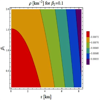
We now perform a graphical check to explore the physical relevancy of the obtained minimally coupled solutions. For this, we plot several physical properties (that have been discussed earlier) which are basically the requirements to be fulfilled. Since there are two parameters involved in the considered modified model along with charge, we adopt their numerical values or ranges to analyze the impact on the stellar models as , and . The question arises here is why we choose these particular values of the model parameters? Haghani and Harko 25ah performed a comprehensive analysis in the context of model I and built some cosmological solutions, i.e., radiation dominated and dust universe. They used different combinations of parametric values such as both positive, both negative or alternative choices, etc. From this, they deduced that the non-negative values of both these parameters provide a best fit with the observational data. So, we initially choose both values and observe that only positive values of yield promising results. For instance, its negative choices produce negative radial pressure near the spherical junction, which is in contrast with the requirement of physically existing compact stellar structures.
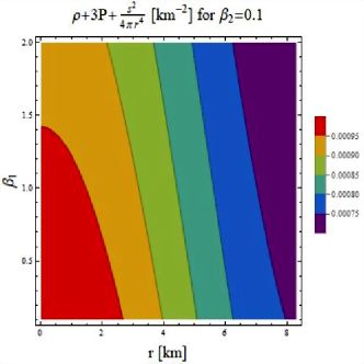
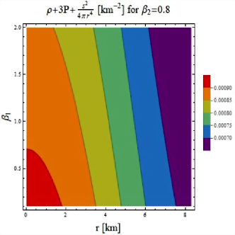
We confirm the behavior of potentials (18) and (19), and found them in agreement with the needed criterion. However, we do not add their plots here. Further, the exploration of the fluid sector (such as isotropic pressure and energy density in this case) is also performed through plotting the corresponding variables in Figures 1 and 2. We notice their required behavior everywhere from the center of a compact star to its boundary surface. From these plotting, we also observe that when the parameters and increase, both the fluid parameters gain less values. This implies that the higher, the values of these parameters, the less dense, the interiors are. The isotropic pressure needs to be null at the spherical interface which is also ensured for each case.
There exist two approaches to calculate the interior mass of any self-gravitating fluid distribution, one in terms of the geometry and other in the form of matter. The former approach is failed to analyze how the modified theory affects the interior mass, therefore, we are left with the later choice (28). We plot this in Figure 3 and find it to be a rising function of . When the parameters and take smaller values, we get the structures with higher mass. Two other factors are also shown in the same Figure, indicating themselves consistent with the required behavior. Figures 4 and 5 admit the positive behavior of energy bounds, naming the developed models as physically viable structures. Finally, both the causality and thermodynamic variations are observed in Figures 6 and 7, indicating the stability of the obtained modified stellar solutions.


IV.2 Model II
This subsection discusses the dynamics of a spherically symmetric interior by adopting a strong non-minimal model of gravity that is given in the following
| (44) |
where the two terms and symbolize arbitrary constants. We adopt a particular form of the functionals and that make the above model as
| (45) |
IV.2.1 Stellar Solution for
Here, we follow the same pattern again as we already discuss in the previous subsection. The equations of motion for the considered geometry are explored for the matter Lagrangian as . Putting this choice with the model (45) in the field equations (11)-(13) and performing some manipulation leads to
| (46) | ||||
| (47) | ||||
| (48) |
Solving last two equations provides the same value of charge as defined in Eq.(38). Further, the isotropic system can be completely characterized by the first two equations, however, it is not possible to find and explicitly due to the appearance of second-order fluid terms. To resolve this issue, we consider a barotropic equation of state represented by
| (49) |
where . After using this equation of state in (46) and (47), we express and as
| (50) | ||||
| (51) |
IV.2.2 Stellar Solution for
Another choice of the matter Lagrangian as is considered that makes Eqs.(11)-(13) when combined with the model (45) as
| (52) | ||||
| (53) | ||||
| (54) |
Simultaneous use of Eqs.(18), (19), (49), (52) and (53) results in the following expressions of and as
| (55) | ||||
| (56) |
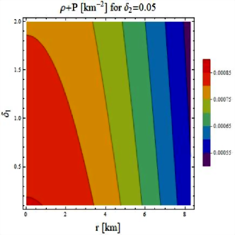
As the graphical exploration for the solution corresponding to model II is concerned, we choose the parametric values as and . It has been observed that only positive values of produce the accelerating solution, but the parameter could either be positive or negative 25ah . However, when we plot physical properties corresponding to our developed solution for its negative choices, the results are not so well behaved. Hence, we are left with positive values of both parameters.
The value of the exterior charge remains same as considered for model I. The same properties (already plotted for the first model) are again explored for this model to check its physical significance in the framework of astronomical structures. Figures 8 and 9 exhibit the profiles of the fluid sector for the above described parametric values, and we observe their acceptable nature. We find that this model produces less dense systems in comparison with the first model for all parametric choices. The factors which are plotted in Figure 3 for model I are again checked for the current scenario and we obtain almost the same results. Therefore, we exclude their graphs from this paper. Further, our model II is also physically viable and this is ensured by the observations which we make in Figures 10 and 11. Lastly, Figures 12 and 13 present the variations in the sound speed and adiabatic index w.r.t. and . It is found that the developed solution only for is stable, however, the model corresponding to the other choice of the Lagrangian density does not fulfill the required criteria.


V Concluding Remarks
This paper discusses multiple isotropic compact models which are coupled with the electromagnetic field in the framework of gravitational theory. For this purpose, we started off with the consideration of a static geometry admitting spherical symmetry and induced an electric charge through the addition of its corresponding Lagrangian in the modified action defined in Eq.(1). We have then implemented the least-action principle on this action and derived the field equations possessing Lagrangian densities of both the fluid and electromagnetic field. It was observed that there are three independent components of equations of motion in the presence of five unknowns, indicated the extra degrees of freedom and thus made it impossible to find a unique solution. This only led to the assumption of some constraints to deal with such issue. In this regard, we have adopted the Karmarkar condition and a particular component form, resulted in computation of the potential such that the ansatz becomes as follows
There are actually three constants in the above ansatz and the constant has been expressed in terms of this triplet as . Therefore, we only needed three conditions which have been provided by the matching conditions at the interface, i.e., in terms of and components. The calculated values of this quartet have been provided in Tables I and II for five distinct compact objects from which we observed the impact of charge on these constants.
We adopted two different (one minimal and one non-minimal) models in this modified context, each of them has been discussed with two different choices of the fluid Lagrangian. The model I contains two parameters which are taken as and . Further, the model II possesses one parameter taken as same as along with an equation of state parameter such as . The fluid doublet has been observed acceptable because it fulfills the required behavior of the energy density and pressure (Figures 1, 2, 8 and 9). We also explored the mass function and reached at the result that the model II possesses less massive interior as compared to the first model for chosen parameters. A necessary condition to be fulfilled is the validity of the energy conditions which has been observed in Figures 4, 5, 10 and 11, hence, our resulting solutions are physically viable. Finally, the stability check has been employed through two different techniques. We have found that the minimal theory yields promising results in the context of astrophysical structures for both and . However, the non-minimal modified model provides stable results only for former choice of the Lagrangian density (Figures 6, 7, 12 and 13). It must be stressed here that disappearing the model parameters reduces all these outcomes in GR.
References
- (1) Capozziello, S. et al.: Class. Quantum Grav. 25(2008) 085004.
- (2) Nojiri, S. et al.: Phys. Lett. B 681(2009)74.
- (3) de Felice, A. and Tsujikawa, S.: Living Rev. Relativ. 13(2010)3.
- (4) Nojiri, S. and Odintsov, S.D.: Phys. Rep. 505(2011)59.
- (5) Astashenok, A.V., Capozziello, S., Odintsov, S.D. and Oikonomou, V.K.: Phys. Lett. B 816(2021)136222.
- (6) Said, J.L. and Adami, K.Z.: Phys. Rev. D 83(2011)043008.
- (7) Astashenok, A.V., Capozziello, S. and Odintsov, S.D.: J. Cosmol. Astropart. Phys. 12(2013)040.
- (8) Naseer, T. and Sharif, M.: Eur. Phys. J. C 84(2024)554.
- (9) Bertolami, O. et al.: Phys. Rev. D 75(2007)104016.
- (10) Naseer, T., Sharif, M., Fatima, A. and Manzoor, S.: Chin. J. Phys. 86(2023)350.
- (11) Harko, T. et al.: Phys. Rev. D 84(2011)024020.
- (12) Deng, X.M. and Xie, Y.: Int. J. Theor. Phys. 54(2015)1739.
- (13) Houndjo, M.J.S.: Int. J. Mod. Phys. D 21(2012)1250003.
- (14) Das, A. et al.: Phys. Rev. D 95(2017)124011.
- (15) Maurya, S.K.: Phys. Dark Universe 30(2020)100640.
- (16) Sharif, M. and Naseer, T.: Eur. Phys. J. Plus 137(2022)1304.
- (17) Sharif, M. and Naseer, T.: Phys. Scr. 98(2023)115012.
- (18) Sharif, M. and Naseer, T.: Ann. Phys. 459(2023)169527.
- (19) Naseer, T. and Sharif, M.: Fortschr. Phys. 72(2024)2300254.
- (20) Feng, Y. et al.: Phys. Scr. 99(2024)085034.
- (21) Naseer, T. and Sharif, M.: Phys. Scr. 99(2024)035001.
- (22) Das, A., Rahaman, F., Guha, B.K. and Ray, S.: Eur. Phys. J. C 76(2016)654.
- (23) Moraes, P.H.R.S., Correa, R.A.C. and Lobato, R.V.: J. Cosmol. Astropart. Phys. 07(2017)029.
- (24) Zaregonbadi, R. et al.: Phys. Rev. D 94(2016)084052.
- (25) Velten, H. and Caramês, T.R.P.: Phys. Rev. D 95(2017)123536.
- (26) Velten, H. and Caramês, T.R.P.: Universe 7(2021)38.
- (27) Haghani, Z. and Harko, T.: Eur. Phys. J. C 81(2021)615.
- (28) Zubair, M., Waheed, S., Muneer, Q. and Ahmad, M.: Fortschr. Phys. 71(2023)2300018.
- (29) Bhar, P. et al.: Eur. Phys. J. A 52(2016)1.
- (30) Maurya, S.K. et al.: Eur. Phys. J. C 76(2016)266.
- (31) Maurya, S.K. et al.: Eur. Phys. J. C 76(2016)693.
- (32) Singh, K.N., Bhar, P. and Pant, N.: Astrophys. Space Sci. 361(2016)1.
- (33) Mustafa, G., Shamir, M.F. and Tie-Cheng, X.: Phys. Rev. D 101(2020)104013.
- (34) Mustafa, G., Tie-Cheng, X. and Shamir, M.F.: Ann. Phys. 413(2020)168059.
- (35) Sharif, M. and Naseer, T.: Phys. Scr. 97(2022)055004.
- (36) Sharif, M. and Naseer, T.: Phys. Scr. 97(2022)125016.
- (37) Feng, Y. et al.: Chin. J. Phys. 90(2024)372.
- (38) Sharif, M. and Naseer, T.: Indian J. Phys. 96(2022)4373.
- (39) Sharif, M. and Naseer, T.: Chin. J. Phys. 81(2023)37.
- (40) Eiesland, J.: Trans. Am. Math. Soc. 27(1925)213.
- (41) Lake, K.: Phys. Rev. D 67(2003)104015.
- (42) Gangopadhyay, T., Ray, S., Xiang-Dong, L., Jishnu, D. and Mira, D.: Mon. Not. R. Astron. Soc. 431(2013)3216.
- (43) Delgaty, M.S.R. and Lake, K.: Comput. Phys. Commun. 115(1998)395.
- (44) Ivanov, B.V.: Eur. Phys. J. C 77(2017)738.
- (45) Sharif, M. and Naseer, T.: Phys. Dark Universe 42(2023)101324.
- (46) Sharif, M. and Naseer, T.: Chin. J. Phys. 86(2023)596.
- (47) Naseer, T. and Sharif, M.: Fortschr. Phys. 71(2023)2300004.
- (48) Sharif, M. and Naseer, T.: Gen. Relativ. Gravit. 55(2023)87.
- (49) Buchdahl, H.A.: Phys. Rev. 116(1959)1027.
- (50) Ivanov, B.V.: Phys. Rev. D 65(2002)104011.
- (51) Abreu, H., Hernandez, H. and Nunez, L.A.: Class. Quantum Grav. 24(2007)4631.
- (52) Heintzmann, H. and Hillebrandt, W.: Astron. Astrophys. 38(1975)51.