Exceptional Points and Stability in Nonlinear Models of Population Dynamics having $\mathcal{PT}$ symmetry

Nonlinear dynamical systems are a widespread, if not ubiquitous, occurrence throughout numerous branches of natural science, with examples ranging from optical and atomic physics Boyd (2008); Besse and Garreau (2015), hydro- and thermodynamics Kirchgassner (1975); Cartwright (2020), to chemical and biological processes Strogatz (2000), population ecology Clark and Luis (2020); Sinervo and Lively (1996); May and Leonard (1975); Kerr et al. (2002), network science Noonburg (1989); Whalen et al. (2015); Szabo and Fath (2006), and socioeconomic systems Barnett et al. (1997); Hauert et al. (2002); Tainaka (1993); Goodwin (1982). Often, already relatively simple nonlinear systems act as cornerstone models that are capable of capturing central qualitative behaviors and features, and give rise to varied phenomenology beyond what can be captured in the linear regime Thompson and Stewart (2002).

In comparison, non-Hermitian – or pseudo-Hermitian – theories have gathered extensive interest rather recently. Commonly traced to the formative work on quantum mechanics with parity-time-reflection ($\mathcal{PT}$) symmetry by Bender and Böttcher Bender and Boettcher (1998), these systems have found particularly fruitful ground in the application to open system dynamics Rotter (2009); Roccati et al. (2022), especially in conjunction with topological features Bergholtz et al. (2021); Kunst et al. (2018); Ding et al. (2022); Okuma and Sato (2022). Here, treating losses due to environmental interactions not as detrimental impediments that are to be minimized and avoided, but instead as advantageous features, which, together with controlled gain, can be beneficial and give rise to novel behaviors, has led to extensive theoretical studies and experimental implementations in various platforms Christodoulides and Yang (2018); Charumathi and Senthilnathan (2024).

Parametric regimes in which nonlinear effects become significant are frequently present in these experiments Ge and El-Ganainy (2016); Ramezani et al. (2010); Musslimani et al. (2008); Malzard et al. (2018); Malzard and Schomerus (2018); Lumer et al. (2013); Smirnova et al. (2020); Ezawa (2022); Yuce (2021); Ma and Susanto (2021); Xia et al. (2021); Wimmer et al. (2015). They outline one natural path to investigations of the interplay between nonlinear dynamics and the features of non-Hermitian systems. Another avenue emerges from applications of $\mathcal{PT}$ symmetry and non-Hermitian topological effects in biological and chemical systems Tang et al. (2021); Nelson and Tang (2024); Zheng and Tang (2024); Bender et al. (2016). Here, oscillatory dynamics are of particular interest, due to their prevalence in natural processes, and stability is of great importance for the self-sustained evolution of many-component systems. In this context, examining the behavior of nonlinear systems through linearized dynamics in the vicinity of stationary states has been connected to the Schrödinger equation of quantum mechanics as a way of accessing results from non-Hermitian physics. The emergence of so-called exceptional points (EPs)–uniquely non-Hermitian singularities–and related non-Hermitian topological properties, such as the non-Hermitian skin effect Bergholtz et al. (2021), have recently been demonstrated in models of evolutionary game theory Yoshida et al. (2021, 2022); Knebel et al. (2020); Liang et al. (2024); Zhang and Cai (2023). This offers a new perspective on natural processes in biological, social, and economic systems through the lens of non-Hermiticity and topology.

However, the linearization approach to stability analysis is ultimately limited to addressing the behavior of the stationary state. While resulting features commonly remain valid in small surrounding domains, the information gained is in general not applicable globally. In this paper, we examine the connection of EPs in local linearizations with the behavior of the underlying nonlinear dynamics for extended evolutionary games of rock-paper-scissors, governed by the replicator equation, and for the topologically related generalized Lotka-Volterra systems originating in population ecology.

When the locally linearized model inherits a global symmetry of the nonlinear system, EP-type phase transitions are found to be indicative of global changes in the nonlinear dynamics, such as an abrupt global destabilization evolving toward the extinction of species or constituents. In contrast, we emphasize that the symmetries central to these non-Hermitian phase transitions, marked by EPs, can emerge as a local feature, disconnected from global symmetries of the full nonlinear theory. In this case, the position of the EP in the linearization decorrelates from the stability transitions of the nonlinear dynamics.

This study is structured as follows. Sections II and III briefly introduce and review the emergence of EPs in the context of evolutionary game theory through the example of the rock-paper-scissors game and $\mathcal{PT}$-symmetric deformations thereof. The stability of the nonlinear dynamics is presented in comparison. By breaking the global symmetry of the model explicitly, differences between local and global symmetries are highlighted. In Secs. IV and V the connection to generalized Lotka-Volterra systems is used to analyze the changes in the global stability through Lyapunov functions, and in VI these behaviors are examined for tri-trophic (that is three-dimensional) iterations of the system. We conclude in Sec. VII.

The game of rock-paper-scissors (RPS) is one of the quintessential mathematical models of game theory Hofbauer and Sigmund (1998). Players choose - rock, paper, or scissors - and compete pairwise: the outcomes are gathered in the so-called payoff matrix of the form

$$A=\,\,\,\blockarray{cccl}\text{R}&\text{P}\text{S}\\ \block{(ccc)l}0-11\,\,\,\,\text{R}\\ 10-1\,\,\,\,\text{P}\\ -110\,\,\,\,\text{S}\\ ,\vspace{-0.4cm}$$

(1)

which represents the success of one player’s pure strategy (in rows) over that of the other (in columns): $1$ represents a win, $0$ a draw, and $-1$ a loss.

In the context of evolution, one imagines a large well-mixed number of players following an initially fixed strategy, which then compete pairwise. For simplicity, we may imagine that after every game the loosing player adopts the winning strategy ¹¹1In general, winning players spawn duplicate players following their strategy according to some growth rate, while loosing players are culled according to some decay rate.. The dynamics of such a game, describing the dissemination of the possible strategies throughout the population of players, are governed by the replicator equation Taylor and Jonker (1978); Hofbauer et al. (1979)

$$\partial_{t}\,x_{i}=x_{i}[(A\mathbf{x})_{i}-\mathbf{x}^{T}A\mathbf{x}]\,,\quad i\in\{R,P,S\}\,,$$

(2)

where $\mathbf{x}$ encodes the frequency of strategies within the total number of players $n$, i.e., $\mathbf{x}=(n_{\text{R}}/n,\,n_{\text{P}}/n,\,n_{\text{S}}/n)$. The standard RPS dynamics are an illustrative example of cyclic dominance Szolnoki et al. (2014), in which the available strategies take turns in being prevalent, leading to cyclicity. At equidistribution of strategies, the dynamics are stationary, $\partial_{t}\mathbf{x}=0$, if not stably so. In fact, the stability of this stationary coexistence point $\bar{\mathbf{x}}_{\text{c}}=(\tfrac{1}{3},\tfrac{1}{3},\tfrac{1}{3})$ is intuitively assessed by examining the dynamical reaction to an added small perturbation $\delta\mathbf{x}$. According to (2), such a disturbance, the tangent flow of the stationary state, evolves as

$$\partial_{t}\,\delta\mathbf{x}\approx\tfrac{1}{3}A\,\delta\mathbf{x}\,.$$

(3)

The solution to this linearization of the nonlinear replicator dynamics (2) thus has the general form of a superposition of the three eigenstates $\mathbf{a}_{j}$ of the matrix $A$:

$$\delta\mathbf{x}(t)=\sum_{j=1}^{3}c_{j}\,\mathbf{a}_{j}\,\mathrm{e}^{\alpha_{j}t/3}\,,\quad\text{$c_{j}$ constant coefficients}\,.$$

(4)

The growth or decay of small disturbances around $\bar{\mathbf{x}}_{c}$ is therefore determined by the nature of the eigenvalues $\alpha_{j}$ of the payoff matrix - with only values having negative real part resulting in a refocusing to the coexistence point. For the standard game of RPS (1), $\alpha_{j}\in\{\pm i\sqrt{3},0\}$, making its coexistence point a center of the linearized dynamics: disturbances neither grow nor decay, but persist. It is thus not asymptotically stable, but for its containment considered to be marginally stable.

This stability analysis of the evolutionary RPS game dynamics based upon a local linearization of the replicator dynamics exemplifies a general and ubiquitous approach to nonlinear models: Lyapunov’s indirect method Kirillov (2013); Wiggins (2010). It is a special example in that the matrix $A$ governing the global dynamics of the system also determines the local linearized dynamics around the coexistence point. This is not generally so; it is, however, linked to the coexistence equilibrium lying at an equidistribution of strategies, which can always be achieved through a rescaling Hofbauer and Sigmund (1998). A major advantage of Lyapunov’s indirect method is the structural simplicity of resulting in a linear first-order partial differential equation, which lends itself readily to analogies with the Schrödinger equation

$$i\partial_{t}\ket{\psi}=H\ket{\psi}$$

(5)

that governs the behavior of wave functions in quantum-mechanical systems.

In Yoshida et al. (2021), the authors draw exactly upon this resemblance to replicate novel behaviors found in the field of non-Hermitian quantum physics within classical population dynamics. Broadly speaking, one there extends models based on conventional Hermitian descriptions, which guarantee entirely real eigenvalues that play the role of an energy spectrum of a persistent physical system, to pseudo-Hermitian models, in which such real energies can also exist, but which furthermore allow for novel phase transitions into regimes with complex eigenvalues Bender (2007); Brody (2013). The mathematical property of pseudo-Hermiticity is frequently associated with the presence of a physical symmetry within the underlying system, such as the seminal $\mathcal{PT}$ symmetry: invariance under combined spacial reflection ($\mathcal{P}$) and time reversal ($\mathcal{T}$) Bender and Boettcher (1998); Bender (2007).

This is clearly illustrated by deforming the standard RPS game in the following way ²²2The model here differs slightly from Yoshida et al. (2022) for clarity, but follows their discussion in keeping with a coexistence point at equidistributed strategies.:

$$A_{\lambda}=\,\,\,\begin{pmatrix}0&-1&1\\ 1&0&-1\\ -1&1&0\end{pmatrix}\,+\,\begin{pmatrix}0&-\lambda&\lambda\\ -\lambda&\lambda&0\\ \lambda&0&-\lambda\end{pmatrix}\,,\quad\lambda\in\mathbb{R}\,.$$

(6)

For positive (negative) values of $\lambda$, the strategy $x_{\text{R}}$ wins more (less) against $x_{\text{S}}$, while $x_{\text{S}}$ loses less (more) against $x_{\text{R}}$. Similarly, $x_{\text{R}}$ loses more (less) against $x_{\text{P}}$, but $x_{\text{P}}$ wins less (more) against $x_{\text{R}}$. The outcomes of $x_{\text{P}}$ playing against $x_{\text{S}}$ remain unchanged, but in the case of a draw of $x_{\text{P}}$ both players obtain a payoff $\lambda$, while for a draw of $x_{\text{S}}$ both players obtain $-\lambda$. Both contributions to this payoff matrix uphold a symmetry of the linearized dynamics, determined by equation (3) with $A_{\lambda}$, under combined time reversal $\mathcal{T}$ ($t\rightarrow-t$) and parity reflection $\mathcal{P}$, in the sense of an exchange of paper and scissors strategies; i.e.,

$$\mathcal{P}=\begin{pmatrix}1&0&0\\ 0&0&1\\ 0&1&0\end{pmatrix}\,,\quad\text{s.t.}\quad\mathcal{P}^{2}=\mathbbm{1}_{3},\quad\mathcal{P}A_{\lambda}\mathcal{P}=-A_{\lambda}\,.$$

(7)

Figure 1 shows the change within the eigenvalues of $A_{\lambda}$ as a function of the deformation strength $\lambda$ and indicates the nature of the equilibrium schematically: The initially imaginary values at $\lambda=0$ transition to appear in real-valued pairs with opposite sign (and an unchanged zero mode) after a critical strength $|\lambda_{\text{EP}}^{\pm}|=1$ is reached. The coexistence point destabilizes from a center at small $\lambda$ to a saddle point beyond the critical values.

This transition reflects a spontaneous breakdown of the underlying $\mathcal{PT}$ symmetry in the linearized system: While the equation of motion (3) is always symmetric, its solutions can lose this symmetry - and after this transition imaginary eigenvalues are no longer protected, see, e.g., Bender (2007); Brody (2013) for in-depth discussions. The critical coupling of this phase transition marks so-called exceptional points having no counterpart in purely (anti-)Hermitian dynamics. They are deficient spectral degeneracies - meaning points of coalescing eigenvalues whose algebraic multiplicity, the number of coinciding eigenvalues, is larger than their geometric multiplicity, the number of linearly independent eigenvectors. A topological $\mathbbm{Z}_{2}$-invariant,

$$\nu=\text{sgn}[\text{Disc}_{\epsilon}\,\text{det}(A_{\lambda}-\epsilon\mathbbm{1})]=\text{sgn}[\lambda^{2}-1]\in\{\pm 1\}\,,$$

(8)

can be attributed to the phases of spontaneously broken ($\nu=1$) and unbroken symmetry ($\nu=-1$) Yoshida et al. (2022).

We remark briefly on the minor difference between the linearized dynamics (3) and the Schrödinger equation (5) that is the appearance of the additional imaginary unit $i$: Due to this factor, stability of quantum systems governed by (5) is commonly associated with real energy eigenvalues of $H$, cf. (4), while this finds its correspondence in imaginary eigenvalues of $A_{\lambda}$ for (3). As such, the simile of Hermitian quantum mechanics is an anti-Hermitian payoff matrix. However, extending this to the pseudo-Hermitian framework, neither matrix will be purely Hermitian nor purely anti-Hermitian - they are generally non-Hermitian. And in both settings, we generally deform an initially stable system to become unstable after some underlying spontaneous symmetry breaking occurs. The transfer of concepts from pseudo-Hermitian quantum physics to the study of nonlinear systems has been applied, e.g., in Ge and El-Ganainy (2016); Ramezani et al. (2010); Musslimani et al. (2008); Malzard et al. (2018); Malzard and Schomerus (2018); Lumer et al. (2013); Smirnova et al. (2020); Ezawa (2022); Yuce (2021); Ma and Susanto (2021). In particular, the prospect of combining many such models within broken symmetry phases to realize the novel phenomenology of non-Hermitian topological states in biological systems has been explored Tang et al. (2021); Nelson and Tang (2024); Zheng and Tang (2024). Nonetheless, these discussions ultimately build upon the linearized behavior within the stability analysis of their nonlinear constituents. However, this linearization is strictly valid only at the stationary position around which the system is perturbed. One may find extended validity within a local domain, that is in a regime of finite but likely only small perturbations - global properties, however, are all but ensured.

While Lyapunov’s indirect method provides a readily accessible technique to analyze the stability of equilibria in nonlinear systems, its meaningfulness relies on identifying the behavior of the nonlinear system with its linearization in the vicinity of a given stationary state. The applicability of this identification is captured in the Hartman-Grobman theorem Wiggins (2010); Hofbauer and Sigmund (1998); Guckenheimer and Holmes (1983), affirming it for hyperbolic equilibria - that is, when no eigenvalue admits a vanishing real part. The coexistence point of the RPS dynamics given by (2) and (3), having a linearization with eigenvalues proportional to $\alpha_{j}\in\{\pm i\sqrt{3},0\}$, thus provides an illustrative example of a non-hyperbolic equilibrium. While we can classify this point as a center of its tangent flow, this does not ensure that it is also a center of the underlying nonlinear dynamics. It might still attract or repel local trajectories sub-exponentially Wiggins (2010). As such, more advanced techniques are required to assess even the behavior in close vicinity of such points, highlighting the precarious nature of transferring concepts from linear to nonlinear systems.

That being said, the RPS coexistence point is in fact also a center of the replicator dynamics, and remains as such under the $\mathcal{PT}$-symmetric deformation (6) up to the critical strength, $|\lambda|<|\lambda_{\text{EP}}|=1$, after which it turns into a saddle point and thus becomes unstable. We will return to the construction of Lyapunov functions that allow to demonstrate such marginal stability of the nonlinear dynamics throughout extended regions in Sec. V.

With a connection between linearized and nonlinear dynamics in the vicinity of the coexistence point present, the non-Hermitian exceptional-point-type phase transition of the linearization also becomes an indicator of structural stability changes of the local nonlinear dynamics. Noting that the $\mathcal{PT}$ symmetry, whose spontaneous breakdown underpins the exceptional point of the linearized system and its parallel to non-Hermitian quantum systems, is moreover a global symmetry of the nonlinear system

$$\partial_{t}\,x_{i}=x_{i}[(A_{\lambda}\mathbf{x})_{i}-\mathbf{x}^{T}A_{\lambda}\mathbf{x}]\,,\quad\text{where}\,\,\,x_{i}=x_{i}(t)\,,$$

(9)

that is to say (9) is obeyed also by

$$\mathbf{x}^{\prime}=\mathcal{PT}\mathbf{x}=\big{(}x_{\text{R}}(-t),x_{\text{S}}(-t),x_{\text{P}}(-t)\big{)}^{T}\,,$$

(10)

we may ask whether the exceptional points in the linearized dynamics can serve as an identifier of global stability changes within the full nonlinear system.

To examine the global behavior of the nonlinear dynamics, we characterize the remaining stationary states of the system: while the coexistence point is a unique equilibrium Hofbauer and Sigmund (1998), the replicator dynamics (9) admit additional boundary equilibria for which at least one type of strategy is not present in the player population. In the standard RPS case ($\lambda=0$) three such points exist, namely the points for which the full player population follows a single strategy:

$$\bar{\mathbf{x}}_{\text{r}}=(1,0,0)^{T}\,,\quad\bar{\mathbf{x}}_{\text{p}}=(0,1,0)^{T}\,,\quad\bar{\mathbf{x}}_{\text{s}}=(0,0,1)^{T}.$$

(11)

The fixed-point nature of these points is ensured by the replicator equation, independent of the payoff matrix, and thus they remain equilibria of the deformed RPS dynamics with $A_{\lambda}$ as well. For $\lambda>1$ or $\lambda<-\frac{1}{2}$ additional stationary states emerge at

$$\bar{\mathbf{x}}_{\text{rp}}=\big{(}\mfrac{2\lambda\!+\!1}{3\lambda},\mfrac{\lambda\!-\!1}{3\lambda},0\big{)}^{T}\,\,\,\text{and}\,\,\,\,\bar{\mathbf{x}}_{\text{rs}}=\big{(}\mfrac{2\lambda\!+\!1}{3\lambda},0,\mfrac{\lambda\!-\!1}{3\lambda}\big{)}^{T}.$$

(12)

In the case of $\lambda<-\frac{1}{2}$, these bifurcate from $\bar{\mathbf{x}}_{\text{p}}$ and $\bar{\mathbf{x}}_{\text{s}}$, respectively, while for $\lambda>1$ they both (pitchfork-)bifurcate from $\bar{\mathbf{x}}_{\text{r}}$, see Fig. 2.

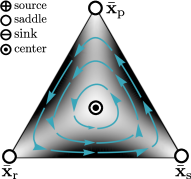
All boundary equilibria are hyperbolic stationary states and straightforwardly classified using Lyapunov’s indirect method to be saddle points, sources, or sinks. Figure 3 shows the behavior of the $\mathcal{PT}$-deformed RPS dynamics on the 2-simplex at representative deformation strengths $\lambda$ with the single-strategy equilibria as vertices. Indicated are in particular the position and nature of all equilibrium points. Notably, the behavior is structurally stable throughout different regimes of deformation, meaning changes in the parameter $\lambda$ do not change the type and stability of the critical points, and trajectories thus remain qualitatively unaffected Wiggins (2010).

In the standard RPS case and for all deformations within $-\frac{1}{2}<\lambda<\lambda_{\text{EP}}^{+}=1$, the boundary equilibria are saddles and the overall behavior follows cyclic dynamics around the center point at the coexistence equilibrium. These dynamics are stable globally (see also Sec. V), cf. Fig. 3c.

For $\lambda<-\frac{1}{2}$, the boundary equilibrium $\bar{\mathbf{x}}_{\text{r}}$ remains a saddle, while $\bar{\mathbf{x}}_{\text{p}}$ and $\bar{\mathbf{x}}_{\text{s}}$ become a sink and a source, respectively. Accordingly, the dynamics can no longer be stable globally. However, both $\bar{\mathbf{x}}_{\text{p}}$ and $\bar{\mathbf{x}}_{\text{s}}$ furthermore bifurcate and give rise to additional boundary equilibria $\bar{\mathbf{x}}_{\text{rp}}$ and $\bar{\mathbf{x}}_{\text{rs}}$, which are saddle points within the regime $-1=\lambda_{\text{EP}}^{-}<\lambda<-\frac{1}{2}$. Here they are connected directly by a separatrix, indicated as dashed line in Fig. 3b, that separates unstable source-sink dynamics at small frequencies $x_{\text{R}}$ of the rock strategy within the player population from stable cyclic dynamics around the center coexistence point. As such, at $\lambda=-\frac{1}{2}$ the global stability of the dynamics continuously transitions to a regime in which extended regional stability of the system is maintained.

Crossing the critical negative value $\lambda_{\text{EP}}^{-}=-1$, the boundary equilibria $\bar{\mathbf{x}}_{\text{rp}}$ and $\bar{\mathbf{x}}_{\text{rs}}$ on the 2-simplex edges change from being saddle points to a source and sink, respectively. The coexistence point destabilizes from a center to a saddle–its stable and unstable manifold, comprising the paths of steepest ascent and descent, form separatrices of the behavior of the system, indicated as dashed lines in Fig. 3a. These separatrices divide the dynamics into four regions, which are characterized by the combinations of sources and sinks that act as beginning and endpoints of all trajectories therein. The dynamics abruptly change from extended regional stability to become globally unstable in the regime $\lambda<\lambda_{\text{EP}}^{-}=-1$: all trajectories evolve toward one of the two sinks on the boundary.

Similarly, beyond the positive critical value, $\lambda>\lambda_{\text{EP}}^{+}=1$, the boundary equilibria $\bar{\mathbf{x}}_{\text{p}}$ and $\bar{\mathbf{x}}_{\text{s}}$ turn from saddles to become a source and a sink, respectively–opposite to their behavior at large negative $\lambda$ values. $\bar{\mathbf{x}}_{\text{r}}$ remains a saddle point, but with reversed ascent and descent paths, and pitchfork-bifurcates to give rise to the additional sink $\bar{\mathbf{x}}_{\text{rp}}$ and source $\bar{\mathbf{x}}_{\text{rs}}$ on the 2-simplex edges, cf. Fig. 4a. The coexistence point destabilizes from a center to a saddle and its stable and unstable manifold again form separatrices of the behavior of the system, indicated as dashed lines in Fig. 3d. The dynamics abruptly become globally unstable in the regime $\lambda>\lambda_{\text{EP}}^{+}=1$.

Overall, one observes that the exceptional-point transitions at $\lambda_{\text{EP}}^{\pm}=\pm 1$ of the linearized dynamics at the coexistence point coincide with abrupt changes in the global stability of the nonlinear system. The regime of spontaneously-broken $\mathcal{PT}$ symmetry of the linearization corresponds to a regime of globally unstable dynamics. In the unbroken $\mathcal{PT}$ symmetry regime of the linearization an additional change in the structural stability of the global dynamics occurs at $\lambda=-\frac{1}{2}$; this change from global stability to extended regional stability, however, is continuous in the sense that the stable region smoothly expands to encompass the full global dynamics at this transition point.

The generalized Lotka-Volterra (GLV) system provides a cornerstone model for the joint evolution of $N$ species populations $y_{i}\in\mathbbm{R}^{\geq 0}$ Hofbauer and Sigmund (1998). Its dynamics are governed by a system of nonlinear first-order differential equations,

$$\partial_{t}y_{i}(t)=r_{i}\,y_{i}(t)+y_{i}(t)\big{[}\sum_{j=1}^{N}b_{ij}\,y_{j}(t)\big{]},$$

(16)

where $r_{i}$ denote the intrinsic growth rates of the species and $b_{ij}$ specify their pairwise interactions. A matrix form is given by

$$\partial_{t}\mathbf{y}(t)=\text{diag}(y_{1}(t),...,y_{N}(t))\,[\mathbf{r}+B\,\mathbf{y}(t)],$$

(17)

where $B=(b_{ij})$ is called the interaction matrix. The pairwise interactions of species may be competitive ($b_{ij}\,\&\,b_{ji}<0$), mutualistic ($b_{ij}\,\&\,b_{ji}>0$), or antagonistic ($b_{ij}b_{ji}<0$, predator-prey type) and self-interactions can be logistic (self-regulating through negative density dependence) for $b_{ii}<0$, or orthologistic (positive density dependence) for $b_{ii}>0$. Such systems admit a large variety of possible dynamical behaviors, including limit cycles, chaotic evolution and stationary fixed points. In particular the cyclic evolution possible in antagonistic models has long been of wide interest in the context of theoretical ecology due to its prevalence in population dynamics and chemical kinetics (self-catalyzing reactions), which provided the foundation for the original two-species model Lotka (1920); Volterra (1926). Today, the GLV system finds widespread application beyond these fields, ranging from neural nets Noonburg (1989); Yi (2010) and plasma physics Laval and Pellat (1975) to economic systems Orlando and Sportelli (2021); Goodwin (1982).

A notable property of the system (16) is the topological equivalence of its dynamics to those of the $(N+1)$-dimensional replicator equation Hofbauer and Sigmund (1998), cf. (2), with a geometric constrain in the sum of frequencies. By supplementing the GLV system with an ancillary variable $y_{0}(t)=1$ and performing a barycentric coordinate transformation $\mathbf{y}(t)\rightarrow\mathbf{x}(t)$ so that:

$$x_{i}(t)=\frac{y_{i}(t)}{\sum_{j=0}^{N}y_{j}}\,,\quad\text{inversely}\quad y_{i}(t)=\frac{x_{i}(t)}{x_{0}}\,,$$

(18)

one arrives at

	$\displaystyle\partial_{t}x_{i}=$	$\displaystyle x_{i}\big{[}\mfrac{\partial_{t}x_{0}}{x_{0}}+\sum_{j=0}^{N}\tilde{B}_{ij}(\mfrac{x_{j}}{x_{0}})\big{]}$		(19)
	$\displaystyle=$	$\displaystyle\mfrac{1}{x_{0}}\{x_{i}\big{[}(\tilde{B}\mathbf{x})_{i}-\mathbf{x}^{T}\tilde{B}\mathbf{x}]\}\,,$		(20)

where the matrix $\tilde{B}$ has the form

$$\tilde{B}=\left(\begin{array}[]{@{}c|c@{}}\,0&\begin{matrix}0&\cdots&0\,\end{matrix}\\ \hline\cr\,\mathbf{r}&B\\ \end{array}\right)\,.$$

(21)

This coincides with the replicator equation up to a scaling of the velocity, that is the trajectories are topologically equivalent to those of the replicator equation with payoff matrix $\tilde{B}$, but they are traversed at different timescales Hofbauer and Sigmund (1998). This embedding of the $N$-dimensional GLV dynamics in an $(N+1)$-dimensional replicator system establishes the correspondence of the models in the context of stability analysis.

One further notes that the structure of the payoff matrix in the replicator equation, cf. (2), has the following ambiguity Hofbauer et al. (1979): The addition of a constant to any column of the payoff matrix,

$$A\rightarrow A^{\prime}=\begin{pmatrix}a_{00}+c_{0}&a_{01}+c_{1}&\cdots&a_{0N}+c_{N}\\ a_{10}+c_{0}&a_{11}+c_{1}&\cdots&a_{1N}+c_{N}\\ \vdots&\vdots&&\vdots\\ a_{N0}+c_{0}&a_{N1}+c_{1}&\cdots&a_{NN}+c_{N}\end{pmatrix}\\ \,,$$

(22)

leaves the replicator dynamics unchanged. As such, any payoff matrix can always be brought into the form (21) and an equivalent GLV system can thus be found. In this sense, the geometrically constrained replicator equation can be regarded as a compactification of the GLV system.

In consequence, the two-dimensional antagonistic GLV system of the form

		$\displaystyle\partial_{t}y_{1}=y_{1}(1+y_{1}-2y_{2}),$		(23)
		$\displaystyle\partial_{t}y_{2}=y_{2}(-1+2y_{1}-y_{2})$

provides a two-variable description that corresponds to the dynamics of the game of rock-paper-scissors (1) on the 2-simplex. Notably, the predator species $y_{2}$ self-regulates due to a logistic self-interaction term and the evolution of the prey species $y_{1}$ contains an orthologistic (positive density dependence) self-interaction term. One again finds a unique coexistence equilibrium, sometimes called rest point, at $\mathbf{y}=(1,1)$, around which the dynamics are governed by the linearization

$$\partial_{t}\,\delta\mathbf{y}\approx B\,\delta\mathbf{y}\quad\text{with}\quad B=\begin{pmatrix}1&-2\\ 2&-1\end{pmatrix}\,.\vspace{-0.1cm}$$

(24)

This behavior is entirely determined by the interaction parameters of the population dynamics model in the interaction matrix $B$ of the full nonlinear system. Note that in this two-variable description, the spurious flat-band solution in the spectrum of the linearization is no longer present.

In addition to linking the evolutionary game theory results to models of population dynamics and thus providing a wider context for non-Hermitian physics in nonlinear systems, the topological equivalence between the replicator and GLV systems allows for the transfer of established approaches between these frameworks. In the following, we utilize this equivalence to determine Liapunov functions that establish stability properties of the models considered. Specifically, we will reexamine the connection between EPs arising in the local dynamics at the coexistence point and global stability properties through this lens.

Determining the stability of an equilibrium point in a nonlinear system can, at times, be challenging. For non-hyperbolic stationary states, the equivalence of the tangent flow and the underlying nonlinear dynamics is not ensured and Lyapunov’s indirect method of investigating the linearization around the equilibrium is unviable. A more robust technique lies in Lyapunov’s direct method Kirillov (2013); Wiggins (2010), which utilizes the analog of a potential function, a so-called Lyapunov function, to establish stability. The existence of such a function $L:\mathbbm{R}^{N}\rightarrow\mathbbm{R}$, satisfying $L(\bar{\mathbf{y}})=0$ and $L(\mathbf{y})>0$ if $\mathbf{y}\neq\bar{\mathbf{y}}$, with $\tfrac{\mathrm{d}}{\mathrm{d}t}L(\mathbf{y})\leq 0$ in a neighborhood of $\bar{\mathbf{y}}$, ensures the marginal stability of the equilibrium point $\bar{\mathbf{y}}$ Wiggins (2010). The difficulty then lies in determining this Lyapunov function, since a general construction remains unknown. However, for many specific cases examples have been established and the connection between the replicator equation and GLV system illustrates how such examples may be transferred in order to assert stability properties.

Following the construction in Sec. IV, the globally $\mathcal{PT}\!$-symmetric deformation (6) of the rock-paper-scissors model of evolutionary game theory is topologically equivalent to the two-dimensional GLV system with growth rates and interaction matrix

$$\mathbf{r}=(1-\lambda,\,\lambda-1)^{T}\quad\text{and}\quad B=\begin{pmatrix}1+2\lambda&-2-\lambda\\ 2+\lambda&-1-2\lambda\end{pmatrix}\,,$$

(25)

that is

		$\displaystyle\partial_{t}y_{1}=y_{1}[(1-\lambda)+(1+2\lambda)y_{1}-(2+\lambda)y_{2}],$		(26)
		$\displaystyle\partial_{t}y_{2}=y_{2}[(\lambda-1)+(2+\lambda)y_{1}-(1+2\lambda)y_{2}].$

Here the dependence on the strategy $x_{\text{R}}$ was eliminated as ancillary variable and the strategies $x_{\text{P}}$ and $x_{\text{S}}$ were transformed to $y_{1}$ and $y_{2}$, compare (18). Accordingly, one again finds the resulting nonlinear system to be globally symmetric under combined time reversal, $\mathcal{T}:t\rightarrow-t$, and parity reflection $\mathcal{P}$, in the sense of an exchange $y_{1}\leftrightarrow y_{2}$; that is

$$\mathcal{P}=\begin{pmatrix}0&1\\ 1&0\end{pmatrix}\,.$$

(27)

A Lyapunov function for this model can be found as follows. Starting from the replicator equation with payoff matrix (6), we utilize the freedom to add constant column contributions, see (22), without changing the dynamics, in order to eliminate the diagonal entries of the matrix:

$$A_{\lambda}\rightarrow A_{\lambda}^{\prime}=\begin{pmatrix}0&-1-2\lambda&1+2\lambda\\ 1-\lambda&0&\lambda-1\\ \lambda-1&1-\lambda&0\end{pmatrix}\\ \,.$$

(28)

In this form the payoff matrix is antisymmetrizable: given the diagonal matrix $D=d\cdot\text{diag}(\tfrac{1+2\lambda}{1-\lambda},1,1)$ with $d\in\mathbbm{R}^{>}$, one finds that

$$(A_{\lambda}^{\prime}D)=-(A_{\lambda}^{\prime}D)^{T}\,.\vspace{-0.1cm}$$

(29)

However, antisymmetrizability necessitates $D$ to be positive, which holds only for $\lambda\in[-\tfrac{1}{2},1]$. In this regime, the replicator equation then admits a constant of motion of the form

$$C(\mathbf{x},\lambda)=\frac{\big{[}x_{\text{R}}\,\big{(}\mfrac{1-\lambda}{1+2\lambda}\big{)}\big{]}^{\tfrac{1-\lambda}{3(1+\lambda)}}\,\,\big{(}x_{\text{P}}\,x_{\text{S}}\big{)}^{\tfrac{1+2\lambda}{3(1+\lambda)}}}{x_{\text{R}}\,(\tfrac{1-\lambda}{1+2\lambda})+x_{\text{P}}+x_{\text{S}}}\,,$$

(30)

compare Kon (2004). This can now be transformed into a constant of motion of the topologically equivalent GLV system (26) using (18), yielding

$$C(\mathbf{y},\lambda)=\frac{(y_{1}\,y_{2})^{\tfrac{1+2\lambda}{3(1+\lambda)}}}{(\tfrac{1-\lambda}{1+2\lambda})+y_{1}+y_{2}}\,\,\big{(}\mfrac{1-\lambda}{1+2\lambda}\big{)}^{\tfrac{1-\lambda}{3(1+\lambda)}}\,.$$

(31)

In general, this establishes a (noncanonical) Hamiltonian structure Wiggins (2010),

$$\dot{\mathbf{y}}=J\,\nabla C(\mathbf{y},\lambda)\,,\quad\text{with}\quad J=\begin{pmatrix}0&f\\ -f&0\end{pmatrix},\vspace{-0.2cm}$$

(32)

where

$$f=\frac{(y_{1}\,y_{2})^{\tfrac{1+2\lambda}{3(1+\lambda)}}\,\big{(}\tfrac{1-\lambda}{1+2\lambda}\big{)}^{\tfrac{1-\lambda}{3(1+\lambda)}}}{3(1+\lambda)\,y_{1}y_{2}\,\big{[}(\tfrac{1-\lambda}{1+2\lambda})+y_{1}+y_{2}\big{]}^{2}}$$

(33)

giving rise to the equations of motion (26). However, this constant of motion has one essential downside: outside the range $\lambda\in[-\tfrac{1}{2},1]$ it becomes a complex-valued function. Since we are interested in constructing a Lyapunov-candidate function based on the constant of motion, finding a real-valued expression is desirable. Nevertheless, this complex nature notably originates in the last factor of (31), which arises as a contribution from the introduction of the ancillary variable in the compactification of the GLV equation to the replicator form, and which thus only contributes as an overall factor. As such, we may drop this contribution without affecting the time-independence of $C(\mathbf{y},\lambda)$. The resulting function is real-valued for all values of $\lambda$, and we can consider it as an energy function of the population dynamics

$$H(\mathbf{y},\lambda)=\frac{(y_{1}\,y_{2})^{\tfrac{1+2\lambda}{3(1+\lambda)}}}{(\tfrac{1-\lambda}{1+2\lambda})+y_{1}+y_{2}}\,.\vspace{-0.1cm}$$

(34)

Based on this Hamiltonian $H$, we can now introduce a Lyapunov-candidate function as

$$L(\mathbf{y},\lambda)=H(\mathbf{1},\lambda)-H(\mathbf{y},\lambda).$$

(35)

Since this function is derived from a constant of motion, $\frac{\mathrm{d}}{\mathrm{d}t}L(\mathbf{y},\lambda)=0$. Figure 6 shows the amplitude of $L(\mathbf{y},\lambda)$ for exemplary values of the deformation strength $\lambda$. In the vanishing-deformation limit $\lambda=0$, see Fig. 6c, this function is globally strictly positive with global minimum at the coexistence equilibrium. It thus establishes the global (marginal) stability of the theory. In fact, this remains the case for any deformation strength with value $\lambda\in[-\tfrac{1}{2},1]$. For $\lambda\in(-1,-\tfrac{1}{2})$, the coexistence equilibrium becomes a local minimum of the function, see Fig. 6b. $L(\mathbf{y},\lambda)$ remains strictly positive in a finite region with the boundary given by the separatrix connecting the two additional boundary saddle points, compare Sec. III. This establishes regional stability around the coexistence equilibrium with a breakdown at large population sizes. For deformation strengths $|\lambda|>1$, see Fig. 6a and Fig. 6d, the function is no longer meeting the requirements of a Lyapunov function, even within a small neighborhood of the coexistence equilibrium, indicating the destabilization of the theory - coinciding with the deformation strength crossing the EP within the linearization.

Overall, the approach using Lyapunov’s direct method confirms the presumed connection between the linearized and nonlinear dynamics in the vicinity of the coexistence point for both the rock-paper-scissors model and for the topologically equivalent two-dimensional GLV system.

While the two-species GLV system captures various interaction types between two constituents, these dynamics are often modified by the presence of further species. This results in potentially extensive interaction networks or, in the context of ecology, food webs Imane et al. (2024). Despite the complexity of such networks in nature, their central dynamical features are commonly controlled by relatively few dominant connections Busiello et al. (2017). Grouping species categorically into trophic levels, indicating their location within a food chain, has also turned out to be a valuable concept that provides a comparability between vastly different ecosystems Yodzis (2001). Three-dimensional models form a fundamental component of these extensive ecosystems and can thus serve as instructive tool for building a mechanistic understanding of ecological dynamics Abdala-Roberts et al. (2019). Moreover, many agricultural ecosystems comprise only simplified biodiversity for which tri-trophic models can be valuable tools with potential application, e.g., in improved pest control strategies Liu et al. (2009). As such, three-species food webs provide essential models for a qualitative understanding of ecological dynamics. They can admit various structures, including (linear) food chains, chains with omnivory, or cyclic food chains.

In this section, we demonstrate the connection between EPs in the linearized dynamics around a coexistence point with changes in global stability for tri-trophic models as an example of its application to higher-dimensional GLV systems. To this end, we introduce the following family of three-species GLV systems with growth rate and interaction matrix of the form:

$$\mathbf{r}=\frac{1}{\mathcal{N}}\,\,(1,0,-1)^{T}\quad\text{and}\quad B=\frac{1}{\mathcal{N}}\,\,\begin{pmatrix}1&(-2\!-\!\delta)&\delta\\ (3\!+\!\delta)&0&(-3\!-\!\delta)\\ -\delta&(2\!+\!\delta)&-1\end{pmatrix}+\frac{\lambda}{\sqrt{3}}\begin{pmatrix}1&-1&0\\ -1&0&1\\ 0&1&-1\end{pmatrix},\quad\text{where}\,\,\mathcal{N}=\sqrt{11+10\delta+3\delta^{2}}\,.$$

(36)

$$\mathbf{y}^{\prime}=\mathcal{PT}\mathbf{y}=\big{(}y_{3}(-t),y_{2}(-t),y_{1}(-t)\big{)}^{T}$$

(38)

is also a solution of the system.

As in Sec. V, we can construct a Lyapunov function by considering the topologically equivalent four-dimensional replicator equation of (36) and use the freedom to add constant column contributions to the corresponding payoff matrix to eliminate its diagonal entries, without changing the dynamics. The resulting matrix is then antisymmetrizable by the diagonal matrix

$$D=d\cdot\mathrm{diag}\Big{(}[1+\lambda\tfrac{\mathcal{N}}{\sqrt{3}}],1,\mfrac{[2+\delta-2\lambda\tfrac{\mathcal{N}}{\sqrt{3}}]}{[2+\delta+\lambda\tfrac{\mathcal{N}}{\sqrt{3}}]},1\Big{)}$$

(39)

as long as all entries are positive. For $\delta\in\{0,\pm 1\}$, this is ensured between $\lambda=-\frac{\sqrt{3}}{\mathcal{N}}$ and $\lambda=(1+\frac{\delta}{2})\frac{\sqrt{3}}{\mathcal{N}}$. This will restrict the regime of deformation strengths $\lambda$ in which this approach results in a global Lyapunov function, as before. The resulting constant of motion based on (39) with $d=[2+\delta+\lambda\tfrac{\mathcal{N}}{\sqrt{3}}]\,/\,[2+\delta-2\lambda\tfrac{\mathcal{N}}{\sqrt{3}}]$ has the form

$$C(\mathbf{x},\lambda)=\frac{\big{[}x_{0}\big{]}^{\big{(}\frac{1}{1+\lambda\frac{\mathcal{N}}{\sqrt{3}}}\big{)}\big{/}\mathcal{M}}\big{[}x_{2}\big{]}^{\big{(}\frac{[2+\delta+\lambda\frac{\mathcal{N}}{\sqrt{3}}]}{[2+\delta-2\lambda\frac{\mathcal{N}}{\sqrt{3}}]}\big{)}\big{/}\mathcal{M}}}{\Big{[}x_{1}+x_{3}+x_{2}\big{(}\frac{[2+\delta+\lambda\frac{\mathcal{N}}{\sqrt{3}}]}{[2+\delta-2\lambda\frac{\mathcal{N}}{\sqrt{3}}]}\big{)}+x_{0}\big{(}\frac{1}{1+\lambda\frac{\mathcal{N}}{\sqrt{3}}}\big{)}\Big{]}\Big{(}\frac{[2+\delta-2\lambda\frac{\mathcal{N}}{\sqrt{3}}]}{[2+\delta+\lambda\frac{\mathcal{N}}{\sqrt{3}}]}\Big{)}}\,\,\Bigg{[}x_{1}x_{3}\Bigg{(}\mfrac{[2+\delta-2\lambda\tfrac{\mathcal{N}}{\sqrt{3}}]}{[2+\delta+\lambda\tfrac{\mathcal{N}}{\sqrt{3}}]}\Bigg{)}^{2}\,\Bigg{]}^{\,1\big{/}\mathcal{M}}\!,$$

(40)

where $\mathcal{M}=\frac{1}{1+\lambda\frac{\mathcal{N}}{\sqrt{3}}}+3\frac{[2+\delta-\lambda\frac{\mathcal{N}}{\sqrt{3}}]}{[2+\delta-2\lambda\frac{\mathcal{N}}{\sqrt{3}}]}$. After dropping the $x_{0}$ component and mapping to the GLV, this then gives rise to the real-valued energy-like function

$$H(\mathbf{y},\lambda)=\frac{\big{[}y_{2}\big{]}^{\big{(}\frac{[2+\delta+\lambda\frac{\mathcal{N}}{\sqrt{3}}]}{[2+\delta-2\lambda\frac{\mathcal{N}}{\sqrt{3}}]}\big{)}\big{/}\mathcal{M}}}{y_{1}+y_{3}+y_{2}\big{(}\frac{[2+\delta+\lambda\frac{\mathcal{N}}{\sqrt{3}}]}{[2+\delta-2\lambda\frac{\mathcal{N}}{\sqrt{3}}]}\big{)}+\big{(}\frac{1}{1+\lambda\frac{\mathcal{N}}{\sqrt{3}}}\big{)}}\,\,\Bigg{[}y_{1}y_{3}\,\Bigg{(}\mfrac{[2+\delta-2\lambda\tfrac{\mathcal{N}}{\sqrt{3}}]}{[2+\delta+\lambda\tfrac{\mathcal{N}}{\sqrt{3}}]}\Bigg{)}^{2}\,\Bigg{]}^{\,1\big{/}\mathcal{M}}\!.$$

(41)

The function $L(\mathbf{y},\lambda)=H(\mathbf{1},\lambda)-H(\mathbf{y},\lambda)$ then provides a Lyapunov function that ensures the marginal stability of the coexistence point and thus the concurrence of the linearized behavior with the nonlinear dynamics in its vicinity for $|\lambda|<|\lambda_{\mathrm{EP}}^{\pm}|=1$. As in the two-dimensional model, the system is stable globally for small deformations $\lambda$, continuously transitions to a regime of regional stability as indicated by the breakdown of the antisymmetrizability of (39), and becomes globally unstable for deformation strengths $|\lambda|>|\lambda_{\mathrm{EP}}^{\pm}|=1$. In this, it replicates the correlation between EPs in the linearized local dynamics of a globally symmetric model and the global destabilization of the nonlinear dynamics in the context of a higher-dimensional system. We illustrate this behavior for the food chain ($\delta=0$), the cyclic food chain ($\delta=1$), and the food chain with omnivory ($\delta=-1$) through the dynamics compacted to the $3$-simplex.

In this study, we have examined the well-established replicator dynamics of the rock-paper-scissors game and the generalized Lotka-Volterra system, being foundational models of evolutionary game theory and population ecology, through the lens of non-Hermitian physics. When linearized around their coexistence equilibrium, these systems are linked to common non-Hermitian models, undergoing spontaneous-symmetry-breaking phase transitions marked by EPs. We have thereby outlined the restriction of this approach to linking nonlinearity and non-Hermiticity: In general, the linear non-Hermitian theory arises as a local description at the equilibrium only and is a priori not connected to the dynamics of the nonlinear system beyond it. In particular, the underlying symmetry, in which the non-Hermitian phase transition behavior and the occurrence of an EP is rooted, can emerge as a local feature of the equilibrium and does not have to be connected to global symmetries of the full nonlinear theory. Moreover, mirroring a non-Hermitian $\mathcal{PT}$-symmetric Schödinger equation in the linearized dynamics of a nonlinear system commonly gives rise to phases of purely imaginary eigenvalues, such that the stationary state is a non-hyperbolic equilibrium. The validity of the linearization as a representative of the underlying nonlinear dynamics is thus not ensured in these cases, potentially disconnecting the linear and nonlinear model completely.

Nonetheless, when this connection is intact and the local symmetry of the linearized model is inherited from a global symmetry of the nonlinear system, the well-known phase-transition behavior of $\mathcal{PT}$ theories may be indicative of global changes in the nonlinear dynamics. We have examined this connection in the context of the two- and three-dimensional Lotka-Volterra system, demonstrating an agreement of the EP with an abrupt global destabilization of the dynamics, in the sense that the system evolves toward a boundary state in which at least one species becomes extinct. With such systems being widely-used foundational models that capture central dynamical qualities in many areas of science, exceptional point structures may offer a new and valuable local characteristic for the understanding of nonlinear dynamics.

We acknowledge funding from the Max Planck Society’s Lise Meitner Excellence Program 2.0.

References

- Boyd (2008) R. W. Boyd, Nonlinear Optics (Academic Press, 2008).
- Besse and Garreau (2015) C. Besse and J.-C. Garreau, Nonlinear Optical and Atomic Systems (Springer Cham, 2015).
- Kirchgassner (1975) K. Kirchgassner, SIAM Review 17, 652 (1975).
- Cartwright (2020) J. Cartwright, Philos. Trans. R. Soc. A 378, 20190534 (2020).
- Strogatz (2000) S. H. Strogatz, Nonlinear Dynamics and Chaos: With Applications to Physics, Biology, Chemistry and Engineering (Westview Press, 2000).
- Clark and Luis (2020) T. Clark and A. Luis, Nat. Ecol. Evol. 4, 1 (2020).
- Sinervo and Lively (1996) B. Sinervo and C. Lively, Nature 380, 240 (1996).
- May and Leonard (1975) R. May and W. Leonard, SIAM J. Appl. Math. 29, 243 (1975).
- Kerr et al. (2002) B. Kerr, M. Riley, M. Feldman, and B. Bohannan, Nature 418, 171 (2002).
- Noonburg (1989) V. W. Noonburg, SIAM J. Appl. Math. 49, 1779 (1989).
- Whalen et al. (2015) A. Whalen, S. Brennan, T. Sauer, and S. Schiff, Phys. Rev. X 5, 011005 (2015).
- Szabo and Fath (2006) G. Szabo and G. Fath, Phys. Rep. 446, 97 (2006).
- Barnett et al. (1997) W. Barnett, A. Medio, and A. Serletis, Macroecon. Dyn. 19, 1749 (1997).
- Hauert et al. (2002) C. Hauert, S. Monte, J. Hofbauer, and K. Sigmund, Science 296, 1129 (2002).
- Tainaka (1993) K. Tainaka, Phys. Lett. A 176, 303 (1993).
- Goodwin (1982) R. M. Goodwin, in Essays in Economic Dynamics (Palgrave Macmillan UK, 1982), pp. 165–170.
- Thompson and Stewart (2002) J. M. T. Thompson and H. B. Stewart, Nonlinear dynamics and chaos (John Wiley & Sons, 2002).
- Bender and Boettcher (1998) C. M. Bender and S. Boettcher, Phys. Rev. Lett. 80, 5243 (1998).
- Rotter (2009) I. Rotter, J. Phys. A: Math. Theor. 42, 153001 (2009).
- Roccati et al. (2022) F. Roccati, G. M. Palma, F. Ciccarello, and F. Bagarello, Open Syst. Inf. Dyn. 29, 2250004 (2022).
- Bergholtz et al. (2021) E. Bergholtz, J. Budich, and F. Kunst, Rev. Mod. Phys. 93, 015005 (2021).
- Kunst et al. (2018) F. Kunst, E. Edvardsson, J. Budich, and E. Bergholtz, Phys. Rev. Lett. 121, 026808 (2018).
- Ding et al. (2022) K. Ding, C. Fang, and G. Ma, Nat. Rev. Phys. 4, 745 (2022).
- Okuma and Sato (2022) N. Okuma and M. Sato, Annu. Rev. Condens. Matter Phys. 14 (2022).
- Christodoulides and Yang (2018) D. Christodoulides and J. Yang, Parity-time Symmetry and Its Applications (Springer Singapore, 2018).
- Charumathi and Senthilnathan (2024) P. R. Charumathi and K. Senthilnathan, Plasmonics pp. 1–22 (2024).
- Ge and El-Ganainy (2016) L. Ge and R. El-Ganainy, Sci. Rep. 6, 24889 (2016).
- Ramezani et al. (2010) H. Ramezani, T. Kottos, R. El-Ganainy, and D. Christodoulides, Phys. Rev. A 82, 043803 (2010).
- Musslimani et al. (2008) Z. Musslimani, K. Makris, R. El-Ganainy, and D. Christodoulides, Phys. Rev. Lett. 100, 030402 (2008).
- Malzard et al. (2018) S. Malzard, E. Cancellieri, and H. Schomerus, Opt. Express 26, 22506 (2018).
- Malzard and Schomerus (2018) S. Malzard and H. Schomerus, New J. Phys. 20, 063044 (2018).
- Lumer et al. (2013) Y. Lumer, Y. Plotnik, M. C. Rechtsman, and M. Segev, Phys. Rev. Lett. 111, 263901 (2013).
- Smirnova et al. (2020) D. Smirnova, D. Leykam, Y. Chong, and Y. Kivshar, Appl. Phys. Rev. 7, 021306 (2020).
- Ezawa (2022) M. Ezawa, Phys. Rev. Res. 4, 013195 (2022).
- Yuce (2021) C. Yuce, Phys. Lett. A 408, 127484 (2021).
- Ma and Susanto (2021) Y.-P. Ma and H. Susanto, Phys. Rev. E 104, 054206 (2021).
- Xia et al. (2021) S. Xia, D. Kaltsas, D. Song, I. Komis, J. Xu, A. Szameit, H. Buljan, K. Makris, and Z. Chen, Science 372, 72 (2021).
- Wimmer et al. (2015) M. Wimmer, A. Regensburger, M.-A. Miri, C. Bersch, D. Christodoulides, and U. Peschel, Nat. Commun. 6, 7782 (2015).
- Tang et al. (2021) E. Tang, J. Agudo-Canalejo, and R. Golestanian, Phys. Rev. X 11, 031015 (2021).
- Nelson and Tang (2024) A. Nelson and E. Tang, Phys. Rev. B 110, 155116 (2024).
- Zheng and Tang (2024) C. Zheng and E. Tang, Nat. Commun. 15, 6453 (2024).
- Bender et al. (2016) C. M. Bender, A. Ghatak, and M. Gianfreda, J. Phys. A Math. 50, 035601 (2016).
- Yoshida et al. (2021) T. Yoshida, T. Mizoguchi, and Y. Hatsugai, Phys. Rev. E 104, 025003 (2021).
- Yoshida et al. (2022) T. Yoshida, T. Mizoguchi, and Y. Hatsugai, Sci. Rep. 12, 560 (2022).
- Knebel et al. (2020) J. Knebel, P. Geiger, and E. Frey, Phys. Rev. Lett. 125, 258301 (2020).
- Liang et al. (2024) J. Liang, Q. Dai, H. Li, H. Li, and J. Yang, Phys. Rev. E 110, 034208 (2024).
- Zhang and Cai (2023) T. Zhang and Z. Cai, Phys. Rev. B 108, 104304 (2023).
- Hofbauer and Sigmund (1998) J. Hofbauer and K. Sigmund, Evolutionary Games and Population Dynamics (Cambridge University Press, 1998).
- Taylor and Jonker (1978) P. D. Taylor and L. B. Jonker, Math. Biosci. 40, 145 (1978).
- Hofbauer et al. (1979) J. Hofbauer, P. Schuster, and K. Sigmund, J. Theor. Biol. 81, 609 (1979).
- Szolnoki et al. (2014) A. Szolnoki, M. Mobilia, L.-L. Jiang, B. Szczesny, A. Rucklidge, and M. Perc, J. R. Soc. Interface 11, 20140735 (2014).
- Kirillov (2013) O. N. Kirillov, Nonconservative Stability Problems of Modern Physics (Berlin, Boston: De Gruyter, 2013).
- Wiggins (2010) S. Wiggins, Introduction to Applied Nonlinear Dynamical Systems and Chaos (Springer New York, NY, 2010).
- Bender (2007) C. M. Bender, Rep. Prog. Phys. 70, 947 (2007).
- Brody (2013) D. Brody, J. Phys. A: Math. Theor. 47, 035305 (2013).
- Guckenheimer and Holmes (1983) J. Guckenheimer and P. Holmes, Nonlinear Oscillations, Dynamical Systems, and Bifurcations of Vector Fields (Springer New York, NY, 1983).
- Hill et al. (2024) L. Hill, L. Gohsrich, J. Fauman, A. Ghosh, K. Kawagoe, P. Del’Haye, and F. K. Kunst, in Advanced Photonics Congress 2024 (Optica Publishing Group, 2024), p. NpTh2D.4.
- Feng et al. (2012) L. Feng, Y.-L. Xu, W. Fegadolli, M.-H. Lu, J. Oliveira, V. Almeida, Y.-F. Chen, and A. Scherer, Nature Mater 12, 108 (2012).
- Lotka (1920) A. Lotka, Proc. Natl. Acad. Sci. U.S.A. 6, 410 (1920).
- Volterra (1926) V. Volterra, Nature 118, 558 (1926).
- Yi (2010) Z. Yi, IEEE Trans. Neural Netw. 21, 494 (2010).
- Laval and Pellat (1975) G. Laval and R. Pellat, in Proceedings of Summer School of Theoretical Physics (Gordon and Breach, New York, 1975).
- Orlando and Sportelli (2021) G. Orlando and M. Sportelli, Growth and Cycles as a Struggle: Lotka-Volterra, Goodwin and Phillips (2021), pp. 191–208.
- Kon (2004) R. Kon, in Hyperbolic Problems, Theory, Numerics and Applications II (Yokohama Publishers, 2004), pp. 109–116.
- Imane et al. (2024) A. Imane, B. Matthieu, H. Maxime, C.and Walid, M. Mylene, M. Francois, N. Jamal, and T. V. Chi, Proc. R. Soc. A. 480, 20230284 (2024).
- Busiello et al. (2017) D. M. Busiello, S. Suweis, J. Hidalgo, and A. Maritan, Sci. Rep. 7, 12323 (2017).
- Yodzis (2001) P. Yodzis, in Encyclopedia of Biodiversity (Second Edition) (Academic Press, 2001), pp. 264–268.
- Abdala-Roberts et al. (2019) L. Abdala-Roberts, A. Puentes, D. Finke, R. Marquis, M. Montserrat, E. Poelman, S. Rasmann, A. Sentis, N. Dam, G. Wimp, et al., Ecol. Lett. 22, 2151 (2019).
- Liu et al. (2009) Y. Liu, D. L. Liu, M. An, Y. Fu, R. S. Zeng, S. M. Luo, H. Wu, and J. Pratley, Ecol. Model. 220, 3241 (2009).