Examples of compact embedded convex $\lambda$ -hypersurfaces

Qing-Ming Cheng, Junqi Lai and Guoxin Wei Qing-Ming Cheng
Department of Applied Mathematics, Faculty of Science, Fukuoka University, 814-0180, Fukuoka, Japan, [email protected] Junqi Lai
School of Mathematical Sciences, South China Normal University, 510631, Guangzhou, China, [email protected] Guoxin Wei
School of Mathematical Sciences, South China Normal University, 510631, Guangzhou, China, [email protected]

Abstract.

In the paper, we construct compact embedded convex $\lambda$ -hypersurfaces which are diffeomorphic to a sphere and are not isometric to a standard sphere. As the special case of our result, we solve Sun’s problem (Int Math Res Not: 11818-11844, 2021). In this sense, one can not expect to have Alexandrov type theorem for $\lambda$ -hypersurfaces.

^†^†footnotetext: The first author was partially supported by JSPS Grant-in-Aid for Scientific Research (B): No.16H03937 and No.22K03303. The third author was partly supported by NSFC Grant No.12171164, GDUPS (2018).

1. Introduction

A hypersurface $\Sigma^{n}\subset\mathbb{R}^{n+1}$ is called a $\lambda$ -hypersurface if it satisfies

(1.1)

H+{\langle}X,\nu{\rangle}=\lambda,

where $\lambda$ is a constant, $X$ is the position vector, $\nu$ is an inward unit normal vector and $H$ is the mean curvature. The notation of $\lambda$ -hypersurfaces were first introduced by Cheng and Wei in [5] (also see [17]). Cheng and Wei [5] proved that $\lambda$ -hypersurfaces are critical points of the weighted area functional with respect to weighted volume-preserving variations. This equation of $\lambda$ -hypersurfaces also arises in the study of isoperimetric problems in weighted (Gaussian) Euclidean spaces, which is a long-standing topic studied in various fields in science. $\lambda$ -hypersurfaces can also be viewed as stationary solutions to the isoperimetric problem in the Gaussian space. For more information on $\lambda$ -hypersurfaces, one can see [5] and [17].

Firstly, we give some examples of $\lambda$ -hypersurfaces. It is well known that there are several special complete embedded solutions to (1.1):

•

hyperplanes with a distance of $|\lambda|$ from the origin,
•

sphere with radius $\frac{-\lambda+\sqrt{\lambda^{2}+4n}}{2}$ centered at origin,
•

cylinders with an axis through the origin and radius $\frac{-\lambda+\sqrt{\lambda^{2}+4(n-1)}}{2}$ .

In [6], Cheng and Wei constructed the first nontrivial example of a $\lambda$ -hypersurface which is diffeomorphic to $\mathbb{S}^{n-1}\times\mathbb{S}^{1}$ by using techniques similar to Angenent [2]. In [18], using a similar method to McGrath [16], Ross constructed a $\lambda$ -hypersurface in $\mathbb{R}^{2n+2}$ which is diffeomorphic to $\mathbb{S}^{n}\times\mathbb{S}^{n}\times\mathbb{S}^{1}$ and exhibits a $SO(n)\times SO(n)$ rotational symmetry. In [15], Li and Wei constructed an immersed $S^{n}$ $\lambda$ -hypersurface using a similar method to [9]. It is quite interesting to find other nontrivial examples of $\lambda$ -hypersurfaces.

Secondly, we introduce some rigidity results about $\lambda$ -hypersurfaces. If $\lambda=0$ , $\langle X,\nu\rangle+H=\lambda=0$ , then $X:\Sigma^{n}\to\mathbb{R}^{n+1}$ is a self-shrinker of mean curvature flow, which plays an important role for study on singularities of the mean curvature flow. Abresch and Langer [1] proved that the only $1$ -dimensional compact embedded self-shrinker is the circle. Huisken [14] proved any compact embedded, and mean convex ( $H\geq 0$ ) self-shrinkers are spheres. Later, Colding and Minicozzi [7] generalized Huisken’s results to the case of complete self-shrinkers.

If $\lambda\neq 0$ , there are relatively few results about $\lambda$ -hypersurfaces. In [5], Cheng and Wei proved that generalized cylinders $\mathbb{S}^{m}\times\mathbb{R}^{n-m}$ , $0\leq m\leq n$ are the only complete embedded $\lambda$ -hypersurfaces with polynomial volume growth in $\mathbb{R}^{n+1}$ if $H-\lambda\geq 0$ and $\lambda(f_{3}(H-\lambda)-S)\geq 0$ , where $f_{3}=\sum_{i,j,k=1}^{n}h_{ij}h_{jk}h_{ki}$ , $S=\sum_{i,j=1}^{n}h_{ij}^{2}$ , $h_{ij}$ denotes the components of the second fundamental form. This classification result generalizes the result of Huisken [14] and Colding and Minicozzi [7].

For $\lambda>0$ , in [13], Heilman proved that convex $n$ -dimensional $\lambda$ -hypersurfaces are generalized cylinders if $\lambda>0$ , which generalized the rigidity result of Colding and Minicozzi [7] to $\lambda$ -hypersurfaces with $\lambda>0$ .

The case $\lambda<0$ is much more complicated. In [12], by using the explicit expressions of the derivatives of the principal curvatures at the non-umbilical points of the surface, Guang obtained that any strictly mean convex $2$ -dimensional $\lambda$ -hypersurfaces are convex if $\lambda\leq 0$ . Later, by using the maximum principle, Lee [11] showed that any compact embedded and mean convex $n$ -dimensional $\lambda$ -hypersurfaces are convex if $\lambda\leq 0$ . In [4], Chang constructed $1$ -dimensional $\lambda$ -curves in $\mathbb{R}^{2}$ , which are not circles. These surprising examples show that $\lambda$ -surfaces behave very differently when $\lambda<0$ compared to the case $\lambda>0$ . New techniques must be introduced to study this phenomenon. We imagine these examples may carry meaningful information in probability theory (also see [19]).

In [19], Sun developed the compactness theorem for $\lambda$ -surface in $\mathbb{R}^{3}$ with uniform $\lambda$ and genus. As the application of the compactness theorem, he also showed a rigidity theorem for convex $\lambda$ -surfaces. In the same paper, he [19] proposed the problem that constructing a compact convex $\lambda$ -surface which is not a sphere (see Question 4.0.4. on page 25, [19]).

In this paper, motivated by [9, 10, 15, 19], we construct nontrivial embedded $\lambda$ -hypersurfaces which are diffeomorphic to $\mathbb{S}^{n}$ and they are not isometric to a standard sphere. As the special case of our result, that is, $n=2$ , we solve Sun’s problem. In fact, we obtain the following theorem:

Theorem 1.1.

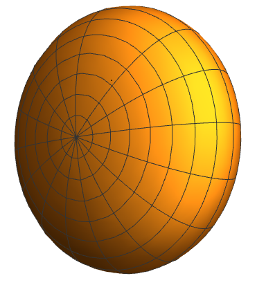
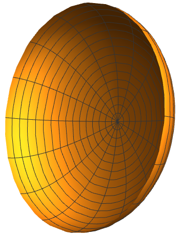
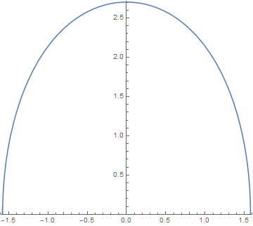
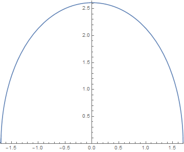
For $n\geq 2$ and $-\frac{2}{\sqrt{n+2}}<\lambda<0$ , there exists an embedded convex $\lambda$ -hypersurface $\Sigma^{n}\subset\mathbb{R}^{n+1}$ which is diffeomorphic to $\mathbb{S}^{n}$ and is not isometric to a standard sphere.

Remark 1.1.

It is well-known that for compact embedded hypersurfaces with constant mean curvature in $\mathbb{R}^{n+1}$ , Alexandrov theorem holds, that is, a compact embedded hypersurface with constant mean curvature in $\mathbb{R}^{n+1}$ is isometric to a round sphere. But for $\lambda$ -hypersurfaces, one can not expect to have Alexandrov type theorem for $\lambda$ -hypersurfaces according to the above theorem 1.1.

Remark 1.2.

For self-shrinkers, there is a well-known conjecture asserts that the round sphere should be the only embedded self-shrinker which is diffeomorphic to a sphere. Brendle [3] proved the above conjecture for $2$ -dimension self-shrinker. For the higher dimensional self-shrinker, the conjecture is still open. But for $\lambda$ -hypersurfaces, we can construct compact embedded $\lambda$ -hypersurface which is diffeomorphic to a sphere and is not isometric to a round sphere.

Remark 1.3.

For $-\frac{2}{\sqrt{3}}<\lambda<0$ , Chang [4] proved that there exists a compact embedded $\lambda$ -curve with $2$ -symmetry in $\mathbb{R}^{2}$ , which is not a circle.

2. Preliminaries

Let $SO(n)$ denote the special orthogonal group and act on $\mathbb{R}^{n+1}=\left\{(x,y):x\in\mathbb{R},y\in\mathbb{R}^{n}\right\}$ in the usual way, then we can identify the space of orbits $\mathbb{R}^{n+1}/SO(n)$ with the half plane $\mathbb{H}=\left\{(x,r)\in\mathbb{R}^{2}:x\in\mathbb{R},r\geq 0\right\}$ under the projection (see [18])

\Pi(x,y)=(x,|y|)=(x,r).

If a hypersurface $\Sigma$ is invariant under the action $SO(n)$ , then the projection $\Pi(\Sigma)$ will give us a profile curve in the half plane, which can be parametrized by Euclidean arc length and write as $\gamma(s)=(x(s),r(s))$ . Conversely, if we have a curve $\gamma(s)=(x(s),r(s)),\ \ s\in(a,b)$ parametrized by Euclidean arc length in the half plane, then we can reconstruct the hypersurface by

	$\displaystyle{X:(a,b)\times S^{n-1}(1)\hookrightarrow\mathbb{R}^{n+1}},$
(2.1)		$\displaystyle(s,\alpha)\mapsto(x(s),r(s)\alpha).$

Let

(2.2)

\nu=(-\dot{r},\dot{x}\,\alpha),

where the dot denotes taking derivative with respect to arc length $s$ . A direct calculation shows that $\nu$ is an inward unit normal vector for the hypersurface. Then we can calculate that the principal curvatures of hypersurface (see [6, 8]):

(2.3)		$\displaystyle\kappa_{i}$	$\displaystyle=-\frac{\dot{x}}{r},\ \ \ \ i=1,\,2,\,\dots,\,n-1,$
(2.3)		$\displaystyle\kappa_{n}$	$\displaystyle=\dot{x}\,\ddot{r}-\ddot{x}\,\dot{r}.$

Hence the mean curvature vector equals to

(2.4)

\overrightarrow{H}=H\nu,\ \ \ \ {\mbox{h}ere}\ \ H=\sum_{i=1}^{n}\kappa_{i}=\dot{x}\,\ddot{r}-\ddot{x}\,\dot{r}-(n-1)\frac{\dot{x}}{r},

and then, by (2.1), (2.2) and (2.4), equation (1.1) reduces to (see also [6, 10, 18])

(2.5)

\dot{x}\,\ddot{r}-\ddot{x}\,\dot{r}=(\frac{n-1}{r}-r)\dot{x}+x\,\dot{r}+\lambda,

where $(\dot{x})^{2}+(\dot{r})^{2}=1$ . Let $\theta(s)$ denote the angles between the tangent vectors of the profile curve and $x$ -axis, then (2.5) can be written as the following system of differential equation:

(2.6)

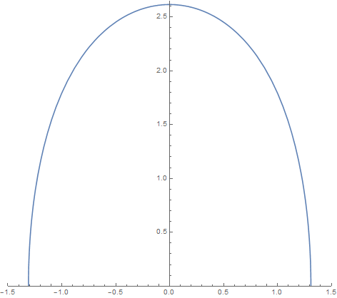
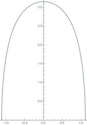
\left\{\begin{aligned} \dot{x}&=\cos\theta,\\ \dot{r}&=\sin\theta,\\ \dot{\theta}&=(\frac{n-1}{r}-r)\cos\theta+x\,\sin\theta+\lambda.\end{aligned}\right.

Let $P$ denote the projection from $\mathbb{H}\times\mathbb{R}$ to $\mathbb{H}$ . Obviously, if $\gamma(s)$ is a solution of (2.6), then the curve $P(\gamma(s))$ will generate a $\lambda$ -hypersurface by (2.1). If we can, by this way, find a curve that starts and ends on the $x$ -axis and is perpendicular to the $x$ -axis at both ends, then we obtain an embedded $\lambda$ -hypersurface, which is diffeomorphic to a sphere. Hence, Theorem 1.1 will be proved. By some symmetry of (2.6), a curve that starts perpendicularly on the $x$ -axis and ends perpendicularly on the $r$ -axis will also solve the problem. This paper’s main goal is to find the latter.
Letting $(x_{0},r_{0},\theta_{0})$ be a point in $\{(x,r,\theta):x\in\mathbb{R},r>0,\theta\in\mathbb{R}\}$ , by an existence and uniqueness theorem of the solutions for first order ordinary differential equations, there is a unique solution $\Gamma(x_{0},r_{0},\theta_{0})(s)$ to (2.6) satisfying initial conditions $\Gamma(x_{0},r_{0},\theta_{0})(0)=(x_{0},r_{0},\theta_{0})$ . Moreover, the solution depends smoothly on the initial conditions. Note that (2.6) has a singularity at $r=0$ due to the term $\frac{1}{r}$ . But there is also an existence and uniqueness theorem for (2.6) with initial conditions at singularity and $\theta_{0}=\pi/2$ . And the previously mentioned smooth dependence can also extend to singularity smoothly (see [9]).

When the profile curve can be written in the form $(x,u(x))$ , by (2.6), the function $u(x)$ satisfies the differential equation

(2.7)

\frac{u^{\prime\prime}}{1+(u^{\prime})^{2}}=x\,u^{\prime}-u+\frac{n-1}{u}+\lambda\sqrt{1+(u^{\prime})^{2}}.

When the profile curve can be written in the form $(f(r),r)$ , by (2.6), the function $f(r)$ satisfies the differential equation

(2.8)

\frac{f^{\prime\prime}}{1+(f^{\prime})^{2}}=(r-\frac{n-1}{r})f^{\prime}-f-\lambda\sqrt{1+(f^{\prime})^{2}}.

Next we consider equations (2.6) in polar coordinates, when the profile curve can be written in the form $\rho=\rho(\phi)$ , where $\rho=\sqrt{x^{2}\,+\,r^{2}}$ and $\phi\,=\,\arctan(r/x)$ , the function $\rho(\phi)$ satisfies the differential equation

(2.9)

\rho^{\prime\prime}\,=\,\frac{1}{\rho}\left\{\rho^{\prime 2}\,+\,(\rho^{2}\,+\,\rho^{\prime 2})\left[n\,-\,\rho^{2}\,-\,(n\,-\,1)\frac{\rho^{\prime}}{\rho}\cot\phi\,-\,\lambda\,\sqrt{\rho^{2}\,+\,\rho^{\prime 2}}\right]\right\}.

Note that (2.8) has a solution $f=-\lambda$ , which corresponds to hyperplane, (2.9) has a solution $\rho\,=\,\frac{-\lambda\,+\,\sqrt{\lambda^{2}\,+\,4\,n}}{2}$ , which corresponds to the round sphere.
We conclude this section with a lemma about the solutions of (2.8), this lemma can be found in [15].

Lemma 2.1 ([15]).

Let $f$ be a solution of (2.8) with $f(0)>-\lambda$ and $f^{\prime}(0)=0$ . Then we have $f^{\prime\prime}<0$ and there exists a point $r_{*}<\infty$ so that $\lim_{r\rightarrow r_{*}}f^{\prime}(r)=-\infty$ and $\lim_{r\rightarrow r_{*}}f(r)>-\infty$ , i.e., $f$ blows-up at $r_{*}$ .

3. Behavior near the known solutions

In order to solve the problem, we need to study the behavior near two known solutions first, and use continuity argument to find the curve that we want to have.

3.1. Behavior near the plane

Let $f_{\epsilon}(r)$ be the solution of (2.8) with $f_{\epsilon}(0)=-\lambda+\epsilon$ and $f_{\epsilon}^{\prime}(0)=0$ where ^′ denotes $\frac{{\rm d}}{{\rm d}r}$ . For $\epsilon>0$ , by Lemma 2.1, let $r_{*}^{\epsilon}$ denote the point where $f_{\epsilon}$ blows-up, and let $x_{*}^{\epsilon}=f_{\epsilon}(r_{*}^{\epsilon})$ . Let $h_{\epsilon}(r)=f_{\epsilon}(r)+\lambda$ , we may write $h_{\epsilon}(r)$ to $h(r)$ , $f_{\epsilon}(r)$ to $f(r)$ , $r_{*}^{\epsilon}$ to $r_{*}$ and $x_{*}^{\epsilon}$ to $x_{*}$ when there is no ambiguity. We introduce the following proposition which gives a description of the behavior near the plane $f_{0}=-\lambda$ .

Proposition 3.1.

For any fixed $n\geq 2$ , $-\min\left\{\frac{23n+4}{28\sqrt{n}},\frac{25n-6}{30\sqrt{n}}\right\}\leq\lambda<0$ , there exists $\bar{\epsilon}>0$ so that

r_{*}^{\epsilon}\geq\sqrt{\log\frac{1}{\sqrt{\pi}\epsilon}},\ \ \ \ -\frac{30n+4}{\sqrt{\log\frac{1}{\sqrt{\pi}\epsilon}}}-\lambda\leq x_{*}^{\epsilon}<-\lambda

for $\epsilon\in(0,\bar{\epsilon}]$ .

To prove the proposition, we need several information on $f_{\epsilon}(r)$ under small $\epsilon$ .

Lemma 3.1.

If $\lambda\leq 0$ , $0<\epsilon\leq\frac{1}{\sqrt{\pi}}$ , then $r_{*}>\sqrt{\log\frac{1}{\sqrt{\pi}\epsilon}}$ .

Proof.

Since $f^{\prime}(0)=0$ , $f^{\prime\prime}(r)<0$ , and $\lim_{r\rightarrow r_{*}}f^{\prime}(r)=-\infty$ , there exists $r^{\prime}\in(0,r_{*})$ so that $f^{\prime}(r^{\prime})=-1$ . Then $h^{\prime}(r^{\prime})$ also equals to $-1$ . For $r\in(0,r^{\prime})$ , we have

	$\displaystyle\dfrac{{\rm d}}{{\rm d}r}(e^{-r^{2}}h^{\prime}(r))$	$\displaystyle=e^{-r^{2}}h^{\prime\prime}(r)-2re^{-r^{2}}h^{\prime}(r)$
		$\displaystyle\geq\dfrac{2}{1+h^{\prime}(r)^{2}}e^{-r^{2}}h^{\prime\prime}(r)-2re^{-r^{2}}h^{\prime}(r)$
		$\displaystyle=2e^{-r^{2}}\left[(r-\dfrac{n-1}{r})h^{\prime}(r)-h(r)+\lambda(1-\sqrt{1+h^{\prime}(r)^{2}})\right]-2re^{-r^{2}}h^{\prime}(r)$
		$\displaystyle\geq-2e^{-r^{2}}h(r),$

where we have used that $\lambda\leq 0$ in the last inequality. Integrating from $0\ {\rm to}\ r^{\prime}$ ,

-e^{-(r^{\prime})^{2}}\geq-2\int_{0}^{r^{\prime}}e^{-r^{2}}h(r){\rm d}r\geq-2\epsilon\int_{0}^{r^{\prime}}e^{-r^{2}}{\rm d}r\geq-\sqrt{\pi}\epsilon.

Hence, we obtain $r_{*}>r^{\prime}\geq\sqrt{\log\frac{1}{\sqrt{\pi}\epsilon}}$ for $\lambda\leq 0$ , $0<\epsilon\leq\frac{1}{\sqrt{\pi}}$ . ∎

Lemma 3.2.

For any fixed $n\geq 2$ , $\lambda\in\mathbb{R}$ , there exists $\epsilon_{1}>0$ so that $f_{\epsilon}(r)=-\lambda$ $($ i.e., $h_{\epsilon}(r)=0$ $)$ has a solution in $[\sqrt{n},\sqrt{2n}]$ for $|\epsilon|\leq\epsilon_{1}$ .

Proof.

We adopt an argument from the appendix B of [10]. In order to understand the behavior of $f_{\epsilon}(r)$ when $\epsilon$ is close to 0, we study the linearization of the rotational $\lambda$ -hypersurface differential equation (2.8) near the plane $f_{0}(r)=-\lambda$ . We define $w$ by

w(r)=\dfrac{{\rm d}}{{\rm d}\epsilon}\bigg{|}_{\epsilon=0}f_{\epsilon}(r).

Since $f_{\epsilon}(r)$ satisfies equation

\dfrac{f_{\epsilon}^{\prime\prime}}{1+(f_{\epsilon}^{\prime})^{2}}=(r-\dfrac{n-1}{r})f_{\epsilon}^{\prime}-f_{\epsilon}-\lambda\sqrt{1+(f_{\epsilon}^{\prime})^{2}},

by differentiating the above equation with respect to $\epsilon$ and letting $\epsilon=0$ , we obtain a differential equation for $w$ :

(3.1)

w^{\prime\prime}=(r-\dfrac{n-1}{r})w^{\prime}-w,

with $w(0)=1$ and $w^{\prime}(0)=0$ , where we have used $f_{0}^{\prime}(r)=0$ . We will show that $w(\sqrt{n})>0$ and $w(\sqrt{2n})<0$ which lead to the lemma.
Defining $\xi=r^{2}$ , the (3.1) becomes into the following differential equation:

(3.2)

4\xi\dfrac{{\rm d}^{2}w}{{\rm d}\xi^{2}}=2(\xi-n)\dfrac{{\rm d}w}{{\rm d}\xi}-w

with the initial conditions at $\xi=0$ :

w(0)=1,\ \ \ \dfrac{{\rm d}w}{{\rm d}\xi}(0)=-\dfrac{1}{2n}.

The equation (3.2) is one of the classical differential equations, namely a confluent hypergeometric equation. Up to a dilation of the argument $\xi$ , the solutions $w$ used here are called Kummer functions. Taking derivatives of (3.2), we have the following second order differential equation:

(3.3)

4\xi\dfrac{{\rm d}^{3}w}{{\rm d}\xi^{3}}=2(\xi-n-2)\dfrac{{\rm d}^{2}w}{{\rm d}\xi^{2}}+\dfrac{{\rm d}w}{{\rm d}\xi}

with the initial conditions at $\xi=0$ :

\dfrac{{\rm d}w}{{\rm d}\xi}(0)=-\dfrac{1}{2n},\ \ \ \dfrac{{\rm d}^{2}w}{{\rm d}\xi^{2}}(0)=-\dfrac{1}{4n(n+2)}.

We also note that the differential equation (3.3) for $\frac{{\rm d}w}{{\rm d}\xi}$ satisfies a maximum principle, which yields that $\frac{{\rm d}^{2}w}{{\rm d}\xi^{2}}<0$ and then $\frac{{\rm d}w}{{\rm d}\xi}\leq\frac{{\rm d}w}{{\rm d}\xi}(0)<0$ . Hence $w$ is strictly concave and strictly decreasing on $[0,\infty)$ . Combining this fact with $w|_{\xi=0}=1$ and $\frac{{\rm d}w}{{\rm d}\xi}(0)=-\frac{1}{2n}$ we obtain $w|_{\xi=2n}<0$ . Let $\xi=n$ in (3.2), we get $w|_{\xi=n}>0$ . Now we have proved that $w|_{\xi=n}>0$ and $w|_{\xi=2n}<0$ , i.e., $w|_{r=\sqrt{n}}>0$ and $w|_{r=\sqrt{2n}}<0$ . ∎

Lemma 3.3.

Suppose $n\geq 2$ , $-\frac{25n-6}{30\sqrt{n}}\leq\lambda<0$ . If there exists a point $r_{0}\in[\sqrt{n},\infty)$ so that $h(r_{0})=0$ , we have

h(r)>\dfrac{30n}{r}h^{\prime}(r)

for $r\in[r_{0},r_{*})$ .

Proof.

Let $\Phi(r)=\frac{1}{30n}rh(r)-h^{\prime}(r)$ . We want to show that $\Phi(r)>0$ for $r\in[r_{0},r_{*})$ . If $r=r_{0}$ , then $\Phi(r_{0})=-h^{\prime}(r_{0})>0$ . If $r>r_{0}$ , by a direct computation, we obtain

	$\displaystyle\Phi(r)$	$\displaystyle=\frac{1}{30n}rh(r)-h^{\prime}(r)$
		$\displaystyle=\dfrac{1}{30n}r\int_{r_{0}}^{r}h^{\prime}(\xi){\rm d}\xi-h^{\prime}(r)$
		$\displaystyle>\dfrac{1}{30n}r(r-r_{0})h^{\prime}(r)-h^{\prime}(r)$
		$\displaystyle=\dfrac{1}{30n}h^{\prime}(r)(r^{2}-r_{0}r-30n)$
		$\displaystyle\geq\dfrac{1}{30n}h^{\prime}(r)(r^{2}-\sqrt{n}r-30n),$

that is, $\Phi(r)>0$ for $r\leq 6\sqrt{n}$ .
Suppose $\Phi(r)=0$ for some $r\in[r_{0},r_{*})$ . Then $r>6\sqrt{n}$ and there exists a point $\bar{r}\in(6\sqrt{n},r_{*})$ so that $\Phi(\bar{r})=0$ and $\Phi(r)>0$ for $r\in[r_{0},\bar{r})$ . This implies that $\Phi^{\prime}(\bar{r})\leq 0$ and $\dfrac{1}{30n}\bar{r}h(\bar{r})=h^{\prime}(\bar{r})$ . On the other hand, since

	$\displaystyle\Phi^{\prime}(\bar{r})$	$\displaystyle=\dfrac{1}{30n}h(\bar{r})+\dfrac{1}{30n}\bar{r}h^{\prime}(\bar{r})-h^{\prime\prime}(\bar{r})$
		$\displaystyle\geq\dfrac{1}{30n}h(\bar{r})+\dfrac{1}{30n}\bar{r}h^{\prime}(\bar{r})-\dfrac{h^{\prime\prime}(\bar{r})}{1+h^{\prime}(\bar{r})^{2}}$
		$\displaystyle=\dfrac{1}{30n}h(\bar{r})+\dfrac{1}{30n}\bar{r}h^{\prime}(\bar{r})-\left[(\bar{r}-\dfrac{n-1}{\bar{r}})h^{\prime}(\bar{r})-f(\bar{r})-\lambda\sqrt{1+h^{\prime}(\bar{r})^{2}}\right]$
		$\displaystyle=\dfrac{1}{30n}h(\bar{r})+\dfrac{1}{30n}\bar{r}h^{\prime}(\bar{r})-\left[(\bar{r}-\dfrac{n-1}{\bar{r}})h^{\prime}(\bar{r})-h(\bar{r})+\lambda(1-\sqrt{1+h^{\prime}(\bar{r})^{2}})\right]$
		$\displaystyle\geq\dfrac{1}{30n}h(\bar{r})+\dfrac{1}{30n}\bar{r}h^{\prime}(\bar{r})-\left[(\bar{r}-\dfrac{n-1}{\bar{r}})h^{\prime}(\bar{r})-h(\bar{r})+\lambda h^{\prime}(\bar{r})\right]$
		$\displaystyle=\dfrac{1}{30n}h(\bar{r})+\dfrac{1}{900n^{2}}\bar{r}^{2}h(\bar{r})-\left[\dfrac{1}{30n}\bar{r}(\bar{r}-\dfrac{n-1}{\bar{r}}+\lambda)h(\bar{r})-h(\bar{r})\right]$
		$\displaystyle=\dfrac{1}{900n^{2}}h(\bar{r})\left[(1-30n)\bar{r}^{2}-30n\lambda\bar{r}+930n^{2}\right]$
		$\displaystyle>0,$

where we have used that $n\geq 2$ , $-\frac{25n-6}{30\sqrt{n}}\leq\lambda<0$ and $\bar{r}>6\sqrt{n}$ in the last inequality, this contradicts $\Phi^{\prime}(\bar{r})\leq 0$ . Hence, we complete the proof. ∎

Proof of Proposition 3.1. The first part of the proposition 3.1 has been shown in the lemma 3.1. We know that $r^{\prime}\geq\sqrt{\log\frac{1}{\sqrt{\pi}\epsilon}}$ for $0<\epsilon\leq\frac{1}{\sqrt{\pi}}$ from the lemma 3.1. In particular, $r^{\prime}\geq\sqrt{\log\frac{1}{\sqrt{\pi}\epsilon}}\geq 7\sqrt{n}$ for $0<\epsilon\leq\frac{1}{\sqrt{\pi}e^{49n}}$ . Choosing $\bar{\epsilon}=\min\left\{\epsilon_{1},\frac{1}{\sqrt{\pi}e^{49n}}\right\}$ and assuming $0<\epsilon\leq\bar{\epsilon}$ , by the lemma 3.2 and lemma 3.3, we have $h(r_{*})<h(r^{\prime})<h(r_{0})=0$ (that is, $x_{*}<-\lambda$ ) and

h(r^{\prime})>-\dfrac{30n}{r^{\prime}}\geq-\dfrac{30n}{\sqrt{\log\frac{1}{\sqrt{\pi}\epsilon}}}.

We will extend this estimate for $h(r^{\prime})$ to an estimate for $h(r_{*})=x_{*}+\lambda$ . For $r\geq r^{\prime}$ , we have

	$\displaystyle h^{\prime\prime}(r)$	$\displaystyle<h^{\prime}(r)^{2}\dfrac{h^{\prime\prime}(r)}{1+h^{\prime}(r)^{2}}$
		$\displaystyle=h^{\prime}(r)^{2}\left[(r-\dfrac{n-1}{r})h^{\prime}(r)-h(r)+\lambda(1-\sqrt{1+h^{\prime}(r)^{2}})\right]$
		$\displaystyle=h^{\prime}(r)^{2}\left[(r-\dfrac{n-1}{r})h^{\prime}(r)-h(r)+\lambda h^{\prime}(r)\right]$
		$\displaystyle<h^{\prime}(r)^{3}(r-\dfrac{31n-1}{r}+\lambda)$
		$\displaystyle\leq\dfrac{1}{4}rh^{\prime}(r)^{3},$

where we have used that $n\geq 2,\ r\geq 7\sqrt{n}$ and $-\frac{23n+4}{28\sqrt{n}}\leq\lambda<0$ in the last inequality.
Integrating the previous inequality from $r$ to $r_{*}$ , implies

h^{\prime}(r)^{2}\leq\dfrac{4}{r_{*}^{2}-r^{2}}

for $r\geq r^{\prime}$ . Since $h^{\prime}(r)<0$ , we have

(3.4)

h^{\prime}(r)\geq-\dfrac{2}{\sqrt{r_{*}^{2}-r^{2}}}\geq-\dfrac{1}{\sqrt{r_{*}+r^{\prime}}}\dfrac{2}{\sqrt{r_{*}-r}}

for $r\in[r^{\prime},r_{*})$ . At $r^{\prime}$ , this tells us that

-\dfrac{\sqrt{r_{*}-r^{\prime}}}{\sqrt{r_{*}+r^{\prime}}}\geq-\dfrac{2}{r_{*}+r^{\prime}}.

Finally, integrating (3.4) from $r^{\prime}$ to $r_{*}$ , we have

h(r_{*})-h(r^{\prime})\geq-\dfrac{4}{\sqrt{r_{*}+r^{\prime}}}\sqrt{r_{*}-r^{\prime}},

and therefore

	$\displaystyle h(r_{*})$	$\displaystyle\geq h(r^{\prime})-\dfrac{4}{\sqrt{r_{}+r^{\prime}}}\sqrt{r_{}-r^{\prime}}$
		$\displaystyle\geq-\dfrac{30n}{r^{\prime}}-\dfrac{8}{r_{*}+r^{\prime}}$
		$\displaystyle\geq-\dfrac{30n+4}{r^{\prime}}$
		$\displaystyle\geq-\frac{30n+4}{\sqrt{\log\frac{1}{\sqrt{\pi}\epsilon}}}.$

Hence $x_{*}\geq-\frac{30n+4}{\sqrt{\log\frac{1}{\sqrt{\pi}\epsilon}}}-\lambda$ , this competes the proof. ∎

3.2. Behavior near the round sphere

As in the proof of the lemma 3.2, we also make use of the method from the appendix B of [10]. Recall equation (2.9), if we can write the profile curve in the form $\rho=\rho(\phi)$ in polar coordinates, where $\rho=\sqrt{x^{2}\,+\,r^{2}}$ and $\phi\,=\,\arctan(r/x)$ , then (2.9) tells us that $\rho=\rho(\phi)$ satisfies

(2.8)

\rho^{\prime\prime}\,=\,\frac{1}{\rho}\left\{\rho^{\prime 2}\,+\,(\rho^{2}\,+\,\rho^{\prime 2})\left[n\,-\,\rho^{2}\,-\,(n\,-\,1)\frac{\rho^{\prime}}{\rho}\cot\phi\,-\,\lambda\,\sqrt{\rho^{2}\,+\,\rho^{\prime 2}}\right]\right\}.

This ordinary differential equation has a constant solution

\rho\,=\,\frac{-\lambda\,+\,\sqrt{\lambda^{2}\,+\,4\,n}}{2}

which corresponds to the round sphere. We note that this equation has a singularity when $\phi=0$ due to the $\cot\phi$ term. Let $\rho(\phi,\epsilon)$ be the solution to (2.8) with initial conditions $\rho(0,\epsilon)=\frac{-\lambda+\sqrt{\lambda^{2}+4\,n}}{2}+\epsilon$ and $\frac{{\rm d}\rho}{{\rm d}\phi}(0,\epsilon)=0$ . As is Drugan and Kleene said in [10], for $\lambda=0$ , the solution $\rho(\phi,\epsilon)$ is smooth when $\phi\in[0,\pi/2]$ and $\epsilon$ is close to 0. This is also true for $\lambda\in\mathbb{R}$ .
In order to understand the behavior of $\rho(\phi,\epsilon)$ when $\epsilon$ is close to 0, we study the linearization of the rotational self-shrinker differential equation near the round sphere $\rho(\phi,0)=\frac{-\lambda+\sqrt{\lambda^{2}+4\,n}}{2}$ . We define $w$ by

w(\phi)=\frac{\rm d}{{\rm d}\epsilon}\bigg{|}_{\epsilon=0}\rho(\phi,\epsilon).

Then $w$ satisfies the (singular) linear differential equation:

(3.5)

w^{\prime\prime}=-(n\,-\,1)\cot\phi\,w^{\prime}\,-\,\frac{-\lambda\,+\,\sqrt{\lambda^{2}\,+\,4\,n}}{2}\,\sqrt{\lambda^{2}\,+\,4n}\,w

with $w(0)=1$ and $w^{\prime}(0)=0$ . Letting $A(\lambda)=\frac{-\lambda\,+\,\sqrt{\lambda^{2}\,+\,4\,n}}{2}\,\sqrt{\lambda^{2}\,+\,4n}$ , we may write $A(\lambda)$ for $A$ when there is no ambiguity. Note that the sign of $A$ is positive for $\lambda\in\mathbb{R}$ . In the following lemma, we claim that $w(\pi/2)<0$ and $w^{\prime}(\pi/2)<0$ which yields that, for $\epsilon<0$ and $\epsilon$ closed to $0$ , $r>\frac{-\lambda\,+\,\sqrt{\lambda^{2}\,+\,4\,n}}{2}$ and $\pi/2<\theta<\pi$ at the first point where the profile curve meets $r$ -axis.

Lemma 3.4.

Let $-\frac{2}{\sqrt{n+2}}<\lambda\leq 0$ , $w$ be the solution to (3.5) with $w(0)=1$ and $w^{\prime}(0)=0$ . Then $w(\pi/2)<0$ and $w^{\prime}(\pi/2)<0$ .

Proof.

By making use of the substitution $\xi=\cos\phi$ , (3.5) becomes into the following Legendre type differential equation:

(3.6)

(1-\xi^{2})\frac{{\rm d}^{2}w}{{\rm d}\xi^{2}}=n\,\xi\,\frac{{\rm d}w}{{\rm d}\xi}-A\,w

with the initial conditions at $\xi=1$ :

w(1)=1,\ \ \ \frac{{\rm d}w}{{\rm d}\xi}(1)=\frac{A}{n}.

To prove the lemma, we need to show that $w=w(\xi)$ satisfies $w(0)<0$ and $\frac{{\rm d}w}{{\rm d}\xi}(0)>0$ .
Taking derivatives of (3.6), we have the following second order differential equations:

(3.7)		$\displaystyle(1-\xi^{2})\frac{{\rm d}^{3}w}{{\rm d}\xi^{3}}=(n+2)\,\xi\,\frac{{\rm d}^{2}w}{{\rm d}\xi^{2}}+(n-A)\,\frac{{\rm d}w}{{\rm d}\xi},$
(3.8)		$\displaystyle(1-\xi^{2})\frac{{\rm d}^{4}w}{{\rm d}\xi^{4}}=(n+4)\,\xi\,\frac{{\rm d}^{3}w}{{\rm d}\xi^{3}}+(2n+2-A)\,\frac{{\rm d}^{2}w}{{\rm d}\xi^{2}}.$

It follows from (3.7) and (3.8) that

\frac{{\rm d}^{2}w}{{\rm d}\xi^{2}}(1)=-\frac{(n-A)A}{n(n+2)},\ \ \ \frac{{\rm d}^{3}w}{{\rm d}\xi^{3}}(1)=\frac{(2n+2-A)(n-A)A}{n(n+2)(n+4)}.

By a direct calculation, we get that $n-A=\frac{1}{2}\lambda(\sqrt{\lambda^{2}+4n}-\lambda)-n<0$ for $\lambda\leq 0$ , and we also get $2n+2-A=-\frac{1}{2}(\lambda^{2}-4-\lambda\sqrt{\lambda^{2}+4n})$ . Then one can obtain $\lambda>-\frac{2}{\sqrt{n+2}}$ by solving inequality $2n+2-A>0$ . Summing up, we have $n-A<0$ and $2n+2-A>0$ for $-\frac{2}{\sqrt{n+2}}<\lambda\leq 0$ , which tell us that $\frac{{\rm d}^{2}w}{{\rm d}\xi^{2}}(1)>0$ and $\frac{{\rm d}^{3}w}{{\rm d}\xi^{3}}(1)<0$ . We also note that the differential equation (3.8) for $\frac{{\rm d}^{2}w}{{\rm d}\xi^{2}}$ satisfies a maximum principle since $2n+2-A>0$ .
Using the same method as in [10], we can obtain $\frac{{\rm d}^{2}w}{{\rm d}\xi^{2}}(0)>0$ and $\frac{{\rm d}^{3}w}{{\rm d}\xi^{3}}(0)<0$ , which follows from (3.6) and (3.7) that $w(0)<0$ and $\frac{{\rm d}w}{{\rm d}\xi}(0)>0$ . Regarding $w=w(\phi)$ as a function of $\phi$ , this says that $w(\pi/2)<0$ and $\frac{{\rm d}w}{{\rm d}\xi}(\pi/2)<0$ , which proves the lemma. ∎

4. Proof of the theorem

Proof of Theorem 1.1. Let $S[x]$ denote the solution to (2.6) with initial conditions $S[x](0)=(x,0,\pi/2)$ . According to the lemma 2.1 we know that, for $x>-\lambda$ , the first component of $P(S[x])$ written as a graph over the $r$ -axis is concave down and decreasing before it blows-up at the point $B_{x}=(f_{x+\lambda}(r_{*}^{x+\lambda}),r_{*}^{x+\lambda})=(x_{*}^{x+\lambda},r_{*}^{x+\lambda})$ . The proposition 3.1 tells us that when $x>-\lambda$ and $x$ closed to $-\lambda$ , $B_{x}$ is in the first quadrant. From the lemma 3.4 we know that when $-\lambda<x<\frac{-\lambda\,+\,\sqrt{\lambda^{2}\,+\,4\,n}}{2}$ and $x$ closed to $\frac{-\lambda\,+\,\sqrt{\lambda^{2}\,+\,4\,n}}{2}$ , $B_{x}$ is in the second quadrant. Since the mapping $(-\lambda,\infty)\rightarrow\mathbb{H},x\mapsto B_{x}$ is continuous, the previous results imply that there exists $\hat{x}\in(-\lambda,\frac{-\lambda\,+\,\sqrt{\lambda^{2}\,+\,4\,n}}{2})$ such that $B_{\hat{x}}$ lies in $r$ -axis. Suppose $P(S[\hat{x}](\hat{s}))=B_{\hat{x}}$ , then the curve $[0,2\hat{s}]\rightarrow\mathbb{H},\,s\mapsto P(S[\hat{x}](s))$ will generate an embedded $\lambda$ -hypersurface by (2.1), which is diffeomorphic to a sphere $\mathbb{S}^{n}$ and is not isometric to the sphere $S^{n}(\frac{-\lambda+\sqrt{\lambda^{2}+4n}}{2})$ . Moreover, by (2.3) and lemma 2.1, all the principal curvatures of the hypersurface we construct is positive. In other words, the hypersurface we construct is convex. ∎

Remark 4.1.

According to some sketches, we know, for $n\geq 2$ and some $\lambda\leq-\frac{2}{\sqrt{n+2}}$ , there exists an embedded $\lambda$ -hypersurface $\Sigma^{n}\subset\mathbb{R}^{n+1}$ which is diffeomorphic to $\mathbb{S}^{n}$ and is not $S^{n}(\frac{-\lambda+\sqrt{\lambda^{2}+4n}}{2})$ (see Figure 4.2, Figure 4.2, Figure 4.4 and Figure 4.4).

Figure 4.1.

n=2,\,\lambda=-1,\,\hat{x}\approx 1.31

Figure 4.2.

n=3,\,\lambda=-0.9,\,\hat{x}\approx 1.11

Refer to caption — Figure 4.3. The graph of the $\lambda$ -hypersurface generated by the profile curve in Figure 4.1

Remark 4.2.

In the proof of Theorem 1.1, we can not assure that the point $\hat{x}$ that we find in $(-\lambda,\frac{-\lambda\,+\,\sqrt{\lambda^{2}\,+\,4\,n}}{2})$ is unique. According to some sketches, for some $n$ and $\lambda<0$ (for example, $n=3$ and $\lambda=-1$ ), there may be more than one points $\hat{x}_{1}$ , $\hat{x}_{2},\cdots$ in $(-\lambda,\frac{-\lambda\,+\,\sqrt{\lambda^{2}\,+\,4\,n}}{2})$ so that

P(S[\hat{x}_{1}](s)),P(S[\hat{x}_{2}](s)),\cdots

will generate embedded $\lambda$ -hypersurfaces by (2.1) (see Figure 4.6 and Figure 4.6).

Figure 4.5.

n=3,\,\lambda=-1,\,\hat{x}\approx 1.57

Figure 4.6.

n=3,\,\lambda=-1,\,\hat{x}\approx 1.69

References

[1] U. Abresch and J. Langer, The normalized curve shortening flow and homothetic solutions, J. Differential Geom. 23 (1986), 175šC196.
[2] S. B. Angenent, Shrinking doughnuts Birkhaüser, Boston-Basel-Berlin, 7, 21-38, 1992.
[3] S. Brendle, Embedded self-similar shrinkers of genus 0, Ann. of Math. 183 (2016), 715-728.
[4] J. -E. Chang, 1-dimensional solutions of the $\lambda$ -self shrinkers, Geom. Dedicata 189 (2017), 97-112.
[5] Q. -M. Cheng and G. Wei, Complete $\lambda$ -hypersurfaces of weighted volume-preserving mean curvature flow, Cal. Var. Partial Differential Equations 57 (2018), 32.
[6] Q. -M. Cheng and G. Wei, Examples of compact $\lambda$ -hypersurfaces in Euclidean spaces, Sci. China Math. 64 (2021), 155-166.
[7] T. H. Colding and W. P. Minicozzi II, Generic mean curvature flow I; generic singularities, Ann. of Math. 175 (2012), 755-833.
[8] M. do Carmo and M. Dajczer, Hypersurfaces in space of constant curvature, Trans. Amer. Math. Soc. 277 (1983), 685-709.
[9] G. Drugan, An immersed $S^{2}$ self-shrinker. Trans. Amer. Math. Soc. 367 (2015), 3139-3159.
[10] G. Drugan and S. J. Kleene, Immersed self-shrinkers, Trans. Amer. Math. Soc. 369 (2017), 7213-7250.
[11] T. -K. Lee, Convexity of $\lambda$ -hypersurfaces, Proc. Amer. Math. Soc. 150 (2022), 1735-1744.
[12] Q. Guang, A note on mean convex $\lambda$ -surfaces in $R^{3}$ , Proc. Amer. Math. Soc. 149 (2021), 1259-1266.
[13] S. Heilman, Symmetric convex sets with minimal Gaussian surface area, Amer. J. Math. 143 (2021), 53-94.
[14] G. Huisken, Asymptotic behavior for singularities of the mean curvature flow, J. Differential Geom. 31 (1990), 285šC299.
[15] Z. Li and G. Wei, An immersed $S^{n}$ $\lambda$ -hypersurface, J. Geom. Anal. 33 (2023), Paper No. 288, 29 pp.
[16] P. McGrath, Closed mean curvature self-shrinking surfaces of generalized rotational type, arXiv: 1507.00681. 2015.
[17] M. McGonagle and J. Ross, The hyperplane is the only stable, smooth solution to the isoperimetric problem in Gaussian space, Geom. Dedicata 178 (2015), 277-296.
[18] J. Ross, On the existence of a closed, embedded, rotational $\lambda$ -hypersurface, J. Geom. 110 (2019), 1-12.
[19] A. Sun, Compactness and rigidity of $\lambda$ -surfaces, Int. Math. Res. Not. IMRN (2021), 11818-11844.

Examples of compact embedded convex λ\lambda-hypersurfaces

Abstract.

1. Introduction

Theorem 1.1.

Remark 1.1.

Remark 1.2.

Remark 1.3.

2. Preliminaries

Lemma 2.1 ([15]).

3. Behavior near the known solutions

3.1. Behavior near the plane

Proposition 3.1.

Lemma 3.1.

Proof.

Lemma 3.2.

Proof.

Lemma 3.3.

Proof.

3.2. Behavior near the round sphere

Lemma 3.4.

Proof.

4. Proof of the theorem

Remark 4.1.

Remark 4.2.

References

Examples of compact embedded convex $\lambda$ -hypersurfaces