^†^†institutetext: Department of Physics & Astronomy
University of Manitoba, Winnipeg, Manitoba R3T 2N2, Canada

Examining Instabilities Due to Driven Scalars in AdS

Abstract

We extend the study of the non-linear perturbative theory of weakly turbulent energy cascades in AdS_d+1 to include solutions of driven systems, i.e. those with time-dependent sources on the AdS boundary. This necessitates the activation of non-normalizable modes in the linear solution for the massive bulk scalar field, which couple to the metric and normalizable scalar modes. We determine analytic expressions for secular terms in the renormalization flow equations mass values $m_{BF}^{2}<m^{2}\leq 0$ , and for various driving functions. Finally, we numerically evaluate these sources for $d=4$ and discuss what role these driven solutions play in the perturbative stability of AdS.

Keywords:

Anti-de Sitter Instability, Gauge/Gravity Duality, Holographic Quantum Quenches

1 Introduction

Nonlinear instabilities in Anti-de Sitter space have been the subject of examinations on several grounds in addition to the holographic description of quantum quenches via the AdS/CFT correspondence 1708.05600 ; 1501.00007 , including general stability of maximally-symmetric solutions in general relativity 1104.3702 ; 1208.5772 ; 1706.06101 , and the study of the growth of secular terms in time-dependent perturbation theories hep-th/9506161 ; 1305.4117 . Numerical studies in AdS show that the eventual collapse of a scalar field into a black hole in the bulk (which is dual to the thermalization of the boundary theory) is generic to any finite sized perturbation 1104.3702 ; 1106.2339 ; 1108.4539 , but can be avoided or delayed for certain initial conditions 1803.02830 ; 1711.00454 ; 1706.07413 ; 1508.02709 . The mechanism of collapse in such systems is described as a weakly turbulent energy cascade to short length scales. These dynamics can be captured by a non-linear perturbation theory at first non-trivial order through the introduction of a second, “slow time” that describes energy transfer between the fundamental modes. This is known as the Two-Time Formalism (TTF) 1403.6471 and yields renormalization flow equations that allow for the absorption of secular terms into renormalized amplitudes and phases 1308.2132 ; 1508.05474 ; 1407.6273 ; 1412.3249 ; 1508.04943 . This way, stability against a perturbation of order $\epsilon$ is maintained over time scales of $t\sim\epsilon^{-2}$ .

Conventional examinations of perturbative stability using TTF have focused on the reaction of the bulk space to some initial energy perturbation, and have aimed to study the balance between direct and inverse energy cascades 1606.02712 ; 1612.04758 ; 1602.05859 ; 1507.08261 ; 1607.08094 . Furthermore, numerical examinations of “pumped” scalars and their implications for thermalization of the dual theory have also been examined 1410.6201 ; 1712.07637 ; 1612.07701 ; 1502.05726 ; 1706.02438 . However, extensions of the perturbative description to include time-dependent sources – corresponding to a driving term on the boundary of the bulk space – remain unaddressed.

With this in mind, we examine the effects that a time-dependent source on the conformal boundary have on the non-linear perturbative theory in the bulk. The introduction of a driving term on the boundary means that we must include a second class of fundamental modes with arbitrary frequencies hep-th/9805171 . Since these solutions will have non-finite inner products over the bulk space, they are known as non-normalizable modes. Non-normalizable modes are identified through the AdS/CFT correspondence with sources coupling to boundary operators hep-th/9802150 ; hep-th/9802109 .

Following the TTF prescription, we expand all fields in powers of a small perturbation $\epsilon$ . At third order in this perturbation, we find expressions for the resonant terms that are responsible for the weakly turbulent transfer of energy to short length scales which will eventually lead to gravitational collapse. The form of the resonant terms depends on the specific physics of the system, as well as possible symmetries between frequencies. While in general types of resonances are able to be removed by frequency shifts, combinations of frequencies that satisfy a resonance condition will produce secular growth that cannot be absorbed by simple frequency shifts. These terms will be absorbed into the definition of slowly-varying integration constants through a set of renormalization flow equations so that the scalar field remains stable against collapse over perturbative timescales.

This paper is organized as follows: section § 2 discusses how the presence of a time-dependent boundary condition on the scalar field results in the activation of non-normalizable modes. We briefly discuss the interpretation of non-normalizable modes within the AdS/CFT correspondence and how their behaviour near the boundary is related to energy fluctuations in the CFT. Furthermore, we specify any restrictions on the form of the resonances that we are considering. In section § 3, we consider a variety of boundary conditions for non-normalizable modes in the bulk. For each choice of boundary condition, we derive analytic expressions for applicable resonances and evaluate these expressions numerically in four spacetime dimensions for different ranges of scalar field masses. Finally, in § 4 we discuss the implications of non-vanishing resonances on slowly-varying amplitudes and phases, and contrast these results with those for static boundary conditions. Whenever values are calculated, the choice of $d=4$ is implied as to draw the most direct comparison to existing literature such as 1412.3249 ; 1407.6273 ; 1508.04943 ; 1606.02712 .

For completeness, we include details of our derivation of the general source term in Appendix A in the boundary time gauge. As an exercise – and to provide explicit expressions for the resonant contributions when the scalar field has non-zero mass – Appendix C contains the calculation of secular terms in the case of a massive scalar field in AdS_d+1 with any mass-squared, up to and including the Breitenlohner-Freedman mass Breitenlohner:1982bm : $m^{2}_{BF}\leq m^{2}$ . We present numerical evidence of the natural vanishing of two of the three resonances, and then examine the effects of mass-dependence on the non-vanishing channel. Finally, Appendix B focuses on additional possible contributions to the source term when the boundary condition is a single non-normalizable mode but with specific values for the frequency.

2 Normalizable and Non-normalizable Modes

Let us consider a spherically symmetric, minimally coupled, massive scalar field on an asymptotically AdS_d+1 spacetime in global coordinates whose metric is given by

\displaystyle ds^{2}

\displaystyle=\frac{L^{2}}{\cos(x)}\left(-A(t,x)e^{-2\delta(t,x)}\,dt^{2}+A^{-1}(t,x)\,dx^{2}+\sin^{2}(x)\,d\Omega^{2}_{d-1}\right)\,,

(1)

where $L$ is the AdS curvature (hereafter set to $1$ ), and the radial coordinate $x\in[0,\pi/2)$ . The dynamics of the system come from the Einstein and Klein-Gordon equations:

\displaystyle G_{\mu\nu}+\Lambda g_{\mu\nu}=8\pi\left(\nabla_{\mu}\phi\nabla_{\nu}\phi-\frac{1}{2}g_{\mu\nu}\left(\nabla^{\rho}\phi\nabla_{\rho}\phi+m^{2}\phi^{2}\right)\right)\quad\text{and}\quad\nabla^{2}\phi-m^{2}\phi=0\,,

(2)

where the cosmological constant $\Lambda$ for AdS given by $\Lambda=-d(d-1)/2$ . Perturbing around static AdS, the scalar field is expanded in odd powers of epsilon

\displaystyle\phi(t,x)=\epsilon\phi_{1}(t,x)+\epsilon^{3}\phi_{3}(t,x)+\ldots

(3)

and the metric functions $A$ and $\delta$ in even powers,

	$\displaystyle A(t,x)$	$\displaystyle=1+\epsilon^{2}A_{2}(t,x)+\ldots$		(4)
	$\displaystyle\delta(t,x)$	$\displaystyle=\epsilon^{2}\delta_{2}(t,x)+\ldots\,.$		(5)

We choose to work in the boundary gauge, where $\delta(t,\pi/2)=0$ , for reasons that we discuss below.

At linear order, $\phi_{1}$ satisfies

	$\displaystyle\partial^{2}_{t}\phi_{1}+\hat{L}\phi_{1}=0\quad\text{and}$	$\displaystyle\quad\phi_{1}(t,x\to\pi/2)=\mathcal{F}(t)\left(\cos(x)\right)^{\Delta^{-}}\,$		(6)
	$\displaystyle\text{where}\;\;\hat{L}$	$\displaystyle\equiv\frac{1}{\mu}(\mu^{\prime}\partial_{x}+\mu\partial^{2}_{x})-\frac{m^{2}}{\cos^{2}(x)}\,,$		(7)

and $\mu\equiv\tan^{d-1}(x)$ . The time-dependent boundary condition for $\phi_{1}$ is the result of the insertion of a driving term in the conformal theory that a function only of time. Parameterizing the scalar field by

\displaystyle\phi_{1}(t,x)=\sum_{I}c_{I}(t)E_{I}(x)

(8)

yields an solution to (6) in the bulk with $c_{I}(t)=a_{I}\cos\left(\omega_{I}t+b_{I}\right)$ as well as an eigenvalue equation for the spatial part

\displaystyle\hat{L}E_{I}(x)=\omega_{I}^{2}E_{I}(x)\,.

(9)

Requiring regularity at the origin we find that hep-th/9805171

\displaystyle E_{I}(x)=K_{I}\left(\cos(x)\right)^{\Delta^{+}}{{}_{2}F_{1}}\left(\frac{\Delta^{+}+\omega_{I}}{2},\frac{\Delta^{+}-\omega_{I}}{2},d/2;\sin^{2}(x)\right),

(10)

where the positive (negative) root of $\Delta(\Delta-d)=m^{2}$ as $\Delta^{+}$ ( $\Delta^{-}$ ). There are two solution for $E_{I}(x)$ at the boundary, denoted $\Phi^{\pm}_{I}(x)$ , that combine to give the solution at the origin (10) through $E_{I}(x)=C_{I}^{+}\Phi^{+}_{I}(x)+C^{-}_{I}\Phi^{-}_{I}(x)$ , where $C^{\pm}_{I}$ are constants that depend on the frequency $\omega_{I}$ and scaling dimension $\Delta^{\pm}$ . By examining each function’s scaling when $x\to\pi/2$ , we see that $\Phi_{I}^{+}$ goes as $(\cos x)^{\Delta^{+}}$ near the boundary and therefore is normalizable; furthermore, $\Phi_{I}^{-}$ goes as $(\cos x)^{\Delta^{-}}$ in this limit and therefore is non-normalizable with respect to the inner product

\displaystyle\langle f(x),g(x)\rangle=\int^{\pi/2}_{0}dx\,\mu(x)f^{\dagger}(x)g(x)\,.

(11)

Matching this behaviour with the time-dependent boundary condition in (6), we see that the non-normalizable modes are the ones that couple to the driving term Nastase . It is important to realize that the general solution for the scalar field in the bulk, (10), contains both normalizable and non-normalizable components.

For special values of the frequencies $\omega_{I}=\omega_{i}=2i+\Delta^{+}$ with $i\in\mathbb{Z}^{+}$ , the solution is purely normalizable and can be written as

\displaystyle E_{I}(x)\Big{|}_{\omega_{I}=\omega_{i}}=e_{i}(x)

\displaystyle=k_{i}\left(\cos(x)\right)^{\Delta^{+}}P_{i}^{(d/2-1,\,\Delta^{+}-d/2)}\left(\cos(2x)\right)\,,

(12)

with the Jacobi polynomials $P^{(a,b)}_{n}(x)$ satisfying ${\langle e_{i}(x),e_{j}(x)\rangle=\delta_{ij}}$ with respect to the inner product (11) when

\displaystyle k_{i}

\displaystyle=2\sqrt{\frac{(i+\Delta^{+}/2)\Gamma(i+1)\Gamma(i+\Delta^{+})}{\Gamma(i+d/2)\Gamma(i+\Delta^{+}-d/2+1)}}\,.

(13)

For consistency with other frequency values, we choose to write all modes in the general form of (10).

Let us now write the first-order part of the scalar field as a sum over both normalizable and non-normalizable modes

	$\displaystyle\phi_{1}(t,x)$	$\displaystyle=\sum_{I}c_{I}(t)E_{I}(x)$
		$\displaystyle=\sum_{j}a_{j}(t)\cos\left(\omega_{i}t+b_{i}(t)\right)e_{j}(x)+\sum_{\alpha}\bar{A}_{\alpha}\cos\left(\omega_{\alpha}t+\bar{B}_{\alpha}\right)E_{\alpha}(x)\,.$		(14)

As we have seen, the addition of a time-dependent boundary condition on the boundary of AdS activates the non-normalizable modes of the scalar field. The values of $\bar{A}_{\alpha}$ and $\bar{B}_{\alpha}$ will be set by the particular form of the driving term, which we impose. This justifies our choice of working in the boundary gauge; the time $t$ is the proper time measured on the boundary, as well as the time scale of oscillations from the driving term. In the simplest example, the driving term on the boundary is a single, periodic function with (non-integer) frequency $\overline{\omega}$ and (constant) amplitude $\mathcal{A}$

\displaystyle\phi_{1}(t,\pi/2)=\mathcal{A}\cos\overline{\omega}t\,.

(15)

In this case, the vanishing of the normalizable modes at the boundary leaves only the non-normalizable part of (2), which collapses into a single term

\displaystyle\sum_{\alpha}\bar{A}_{\alpha}\cos(\omega_{\alpha}t+\bar{B}_{\alpha})E_{\alpha}(\pi/2)=\mathcal{A}\cos\overline{\omega}t\>\>\Rightarrow\>\>\bar{A}_{\overline{\omega}}\,E_{\overline{\omega}}(\pi/2)=\mathcal{A}\quad\text{and}\quad\bar{B}_{\overline{\omega}}=0\,.

(16)

In practice, we generalize the boundary condition to a sum over Fourier modes $\overline{\omega}_{\alpha}$ , which means that additional $\bar{A}_{\alpha}$ and $\bar{B}_{\alpha}$ terms are non-zero. Note that the allowed non-normalizable frequencies are completely set by the form of the boundary term being considered. In subsequent sections, we will examine several specific choices of driving frequencies that would produce resonances beyond first order. Note that because the non-normalizable frequencies are not restricted to integer values like the normalizable modes, there are an infinite set of possible boundary configurations that could be explored. Therefore, we will restrict our work to a set of configurations that will be particularly useful in comparing to existing work with driven CFTs 1712.07637 ; 1502.05726 ; 1612.07701 ; 1805.00031 .

2.1 Interpretation Through the AdS/CFT Dictionary

The AdS/CFT dictionary relates the leading coefficient of the normalizable modes of the scalar field at the boundary to the expectation value of an operator $\langle\mathcal{O}_{0}\rangle$ there hep-th/9808017 . Similarly, the leading coefficient of the non-normalizable modes is related to a source in the boundary CFT. To illustrate this, consider the leading-order behaviour of the scalar field near the conformal boundary:

\displaystyle\phi\sim\alpha(t)\left(\cos(x)\right)^{\Delta^{-}}+\beta(t)\left(\cos(x)\right)^{\Delta^{+}}+~{}\ldots\,,

(17)

where $\alpha(t)$ and $\beta(t)$ are the coefficients of the non-normalizable and normalizable modes, respectively, as determined by their scaling with $x$ , and the $(\ldots)$ represent subleading contributions. The Hamiltonian on the boundary receives an extra contribution from the operator $\mathcal{O}_{0}$ that goes like

\displaystyle H=H_{CFT}+\alpha(t)\mathcal{O}_{0}\,.

(18)

Therefore, the presence of non-normalizable modes corresponds to a time-dependent portion of the energy of the boundary theory.

In principle, we can determine the exact form of the time dependence of the energy density in the boundary theory in terms of bulk variables. However, there are additional considerations that arise due to non-normalizable modes. In particular, the boundary CFT must be renormalizable and surface terms from the bulk action may contain contributions from non-normalizable modes that violate renormalizability. The process of holographic renormalization can be approached through the explicit calculation of the required counterterms hep-th/9804058 ; hep-th/0112119 , or by rewriting the metric near the boundary in the Fefferman-Graham form 0707.1737 ; hep-th/0303164 ; hep-th/0205075 ; fefferman1985mathematical . However, this process is complicated by the appearance of different terms when either even or odd numbers of dimensions are considered hep-th/0205061 ; 1206.6785 . For these reasons, explicit calculations of one-point functions on the boundary in terms of the bulk variables – which requires that the relevant counterterms be added – will be left to future work.

2.2 The General Source Term

Without specifying whether frequencies or basis functions have been chosen to be either normalizable or non-normalizable for the time being, we can show that the $\mathcal{O}(\epsilon^{3})$ part of the scalar field satisfies the equation

\displaystyle\ddot{\phi}_{3}+\hat{L}\phi_{3}=S=2(A_{2}-\delta_{2})\ddot{\phi}_{1}+(\dot{A}_{2}-\dot{\delta}_{2})\dot{\phi}_{1}+(A_{2}^{\prime}-\delta_{2}^{\prime})\phi_{1}^{\prime}+m^{2}A_{2}\phi_{1}\sec^{2}x\,.

(19)

Following the steps outlined in Appendix A, we project (19) onto the basis of normalizable modes. Since all non-normalizable contributions have been fixed by the $\mathcal{O}(\epsilon)$ boundary condition, there will be no contribution from non-normalizable modes at this order. Using the expansion from (2), we see that ${\langle\phi_{3},e_{\ell}\rangle=c^{(3)}_{\ell}}$ and so

\displaystyle\ddot{c}^{(3)}_{\ell}+\omega_{\ell}^{2}c^{(3)}_{\ell}=S_{\ell}\,.

(20)

As discussed in 1407.6273 , the solution to (20) will contain terms proportional to

\displaystyle\cos(\theta_{I}\pm\theta_{J}\pm\theta_{K})=\cos\left((\omega_{I}\pm\omega_{J}\pm\omega_{K})t+b_{I}\pm b_{J}\pm b_{K}\right)\,.

(21)

For choices of $\{\theta_{I},\theta_{J},\theta_{K}\}$ such that ${\pm\omega_{\ell}\neq\pm\omega_{I}\pm\omega_{J}\pm\omega_{K}}$ , $S_{\ell}$ will always be made up of terms of the form in (21). However, if the frequencies are resonant, i.e. if ${\pm\omega_{\ell}=\pm\omega_{I}\pm\omega_{J}\pm\omega_{K}}$ , then the solution to (20) will contain terms of the form

\displaystyle t\sin(\theta_{I}\pm\theta_{J}\pm\theta_{K})\,.

(22)

These terms, known as secular terms, grow linearly with time and will eventually invalidate the perturbative expansion. While secular terms from non-resonant spectra are able to be absorbed into a shift of $\omega_{\ell}$ , secular terms from fully resonant spectra are not able to be absorbed in this way. Instead, a resummation of secular terms must be applied. Since non-secular terms and secular terms from non-resonant spectra can be controlled for without the use of a resummation scheme, we henceforth let $S_{\ell}$ denote only secular terms from fully resonant spectra since it is these terms that will determine the evolutions of the first-order amplitudes and phases hep-th/9506161 .

The resummation of secular terms can be achieved through either the Two-Time Formalism picture 1403.6471 or the renormalization group resummation picture 1412.3249 . The effect of either method is that we can rewrite the amplitudes and phases in terms of renormalized integration constants that exactly cancel the secular terms at each instant. Doing so yields the renormalization flow equations for the renormalized constants 1407.6273

	$\displaystyle\frac{2\omega_{\ell}}{\epsilon^{2}}\frac{da_{\ell}}{dt}$	$\displaystyle=-\sum_{I,J,K}S_{\ell}\sin\left(b_{\ell}\pm b_{I}\pm b_{J}\pm b_{K}\right)$		(23)
	$\displaystyle\frac{2\omega_{\ell}a_{\ell}}{\epsilon^{2}}\frac{db_{\ell}}{dt}$	$\displaystyle=-\sum_{I,J,K}S_{\ell}\cos\left(b_{\ell}\pm b_{I}\pm b_{J}\pm b_{K}\right)\,,$		(24)

where the sums over ${\{I,J,K\}}$ now only include combinations that give resonant spectra. Note that the amplitudes and phases evolve with respect to the “slow time” $\tau=\epsilon^{2}t$ . In practice, once these flow equations can be written down, the perturbative evolution of the system is determined up to a timescale of $t\sim\epsilon^{-2}$ .

Returning to the result of projecting (19) onto the basis of normalizable modes, we find that the source term for the $\ell^{\rm th}$ mode is

$\displaystyle S_{\ell}$	$\displaystyle=\frac{1}{4}\sum_{\begin{subarray}{c}I,J,K\\ K\neq\ell\end{subarray}}^{\infty}\frac{a_{I}a_{J}a_{K}\omega_{K}}{\omega_{\ell}^{2}-\omega_{K}^{2}}\bigg{[}Z^{-}_{IJK\ell}(\omega_{I}+\omega_{J}-2\omega_{K})\cos(\theta_{I}+\theta_{J}-\theta_{K})$
	$\displaystyle\qquad\frac{}{}-Z^{-}_{IJK\ell}(\omega_{I}+\omega_{J}+2\omega_{K})\cos(\theta_{I}+\theta_{J}+\theta_{K})+Z^{+}_{IJK\ell}(\omega_{I}-\omega_{J}+2\omega_{K})\cos(\theta_{I}-\theta_{J}+\theta_{K})$
	$\displaystyle\qquad\frac{}{}-Z^{+}_{IJK\ell}(\omega_{I}-\omega_{J}-2\omega_{K})\cos(\theta_{I}-\theta_{J}-\theta_{K})\bigg{]}$
	$\displaystyle+\frac{1}{2}\sum_{\begin{subarray}{c}I,J,K\\ I\neq J\end{subarray}}^{\infty}a_{I}a_{J}a_{K}\omega_{J}\left(H_{IJK\ell}+m^{2}V_{JKI\ell}-2\omega_{K}^{2}X_{IJK\ell}\right)\bigg{[}\frac{1}{\omega_{I}-\omega_{J}}\big{(}\cos(\theta_{I}-\theta_{J}-\theta_{K})$
	$\displaystyle\qquad+\cos(\theta_{I}-\theta_{J}+\theta_{K})\big{)}-\frac{1}{\omega_{I}+\omega_{J}}\big{(}\cos(\theta_{I}+\theta_{J}-\theta_{K})+\cos(\theta_{I}+\theta_{J}+\theta_{K})\big{)}\bigg{]}$
	$\displaystyle-\frac{1}{4}\sum_{I,J,K}^{\infty}a_{I}a_{J}a_{K}\bigg{[}\left(2\omega_{J}\omega_{K}X_{IJK\ell}+m^{2}V_{IJK\ell}\right)\cos(\theta_{I}+\theta_{J}-\theta_{K})$
	$\displaystyle\qquad\frac{}{}-\left(2\omega_{J}\omega_{K}X_{IJK\ell}-m^{2}V_{IJK\ell}\right)\cos(\theta_{I}-\theta_{J}-\theta_{K})+\left(2\omega_{J}\omega_{K}X_{IJK\ell}+m^{2}V_{IJK\ell}\right)\cos(\theta_{I}-\theta_{J}+\theta_{K})$
	$\displaystyle\qquad\frac{}{}-\left(2\omega_{J}\omega_{K}X_{IJK\ell}-m^{2}V_{IJK\ell}\right)\cos(\theta_{I}+\theta_{J}+\theta_{K})\bigg{]}$
	$\displaystyle+\frac{1}{4}\sum_{I,J}^{\infty}a_{I}a_{J}a_{\ell}\omega_{\ell}\Big{[}\tilde{Z}^{-}_{IJ\ell}(\omega_{I}+\omega_{J}-2\omega_{\ell})\cos(\theta_{I}+\theta_{J}-\theta_{\ell})-\tilde{Z}^{-}_{IJ\ell}(\omega_{I}+\omega_{J}+2\omega_{\ell})\cos(\theta_{I}+\theta_{J}+\theta_{\ell})$
	$\displaystyle\qquad+\tilde{Z}^{+}_{IJ\ell}(\omega_{I}-\omega_{J}+2\omega_{\ell})\cos(\theta_{I}-\theta_{J}+\theta_{\ell})-\tilde{Z}^{+}_{IJ\ell}(\omega_{I}-\omega_{J}-2\omega_{\ell})\cos(\theta_{I}-\theta_{J}-\theta_{\ell})\Big{]}$
	$\displaystyle-\frac{1}{4}\sum_{I,J}^{\infty}a_{I}^{2}a_{J}\bigg{[}H_{IIJ\ell}+m^{2}V_{JII\ell}-2\omega_{J}^{2}X_{IIJ\ell}\bigg{]}\big{(}\cos(2\theta_{I}-\theta_{J})+\cos(2\theta_{I}+\theta_{J})\big{)}$
	$\displaystyle-\frac{1}{2}\sum_{I,J}^{\infty}a_{I}^{2}a_{J}\bigg{[}H_{IIJ\ell}+m^{2}V_{JII\ell}-2\omega_{J}^{2}X_{IIJ\ell}+4\omega_{I}^{2}\omega_{J}^{2}P_{J\ell I}+2\omega_{I}^{2}(M_{J\ell I}+m^{2}Q_{J\ell I})\bigg{]}\cos\theta_{J}.$	(25)

Note that sums and restrictions on indices must be interpreted as sums and restrictions on frequencies when any of the modes is non-normalizable, since $\omega_{\alpha}\neq 2\alpha+\Delta^{+}$ in general.

2.3 The Resonance Condition

To determine the form of the secular terms in $S_{\ell}$ , we must consider all combinations of the frequencies ${\{\omega_{I},\omega_{J},\omega_{K}\}}$ that satisfy the resonance condition

\displaystyle\omega_{I}\pm\omega_{J}\pm\omega_{K}=\pm\omega_{\ell}\,.

(26)

The allowed values of the non-normalizable frequencies are set by the form of driving term in $\mathcal{F}(t)$ , i.e. which non-normalizable modes have been excited. For instance, if the driving term is of the form in (15), then $\omega_{I}=\{\omega_{i},\overline{\omega}\}$ . Plugging this restriction into (26), we could potentially have resonances from

$\displaystyle\omega_{i}\pm\omega_{j}\pm\overline{\omega}$	$\displaystyle=\pm\omega_{\ell}$	(27)
$\displaystyle\omega_{i}\pm\overline{\omega}\pm\overline{\omega}$	$\displaystyle=\pm\omega_{\ell}$	(28)
$\displaystyle\overline{\omega}\pm\overline{\omega}\pm\overline{\omega}$	$\displaystyle=\pm\omega_{\ell}\,.$	(29)

Since the frequencies of the normalizable modes are always $\omega_{i}=2i+\Delta^{+}$ , and since the non-normalizable modes have generically non-integer frequencies, (27) and (29) require specific values of $\overline{\omega}$ to be satisfied. There is only a single non-trivial resonance that can occur without tuning the value of $\overline{\omega}$ , which is $\omega_{i}+\overline{\omega}-\overline{\omega}=\omega_{\ell}$ . As an additional example, consider the choice of ${\omega_{I}=\omega_{J}=\omega_{K}=\overline{\omega}=2n-\Delta^{-}}$ with $n\in\mathbb{Z}^{+}$ in (26). One resonance that arises from the condition (29) is

\displaystyle\omega_{I}\pm\omega_{J}\pm\omega_{K}=\pm\omega_{\ell}\;\to\;\overline{\omega}-\overline{\omega}+\overline{\omega}=\omega_{\ell}

(30)

which – when working in an even number of dimensions with $d\geq 4$ – is satisfied for $n=\ell-d/2$ . Again, this requires the frequency of the boundary condition to be tuned to a special value.

In the interest of examining the most generic choices for the driving frequency, we do not consider cases that rely on specially tuned values. In particular, we focus on resonances produced when only two of the frequencies in (26) are non-normalizable. Therefore, an important caveat to this work is that it does not present an exhaustive list of possible resonances, and that specific choices for the number of dimensions, mass, and driving frequency could result in cases not addressed here. In fact, tuning the frequency of the boundary condition may lead to some very interesting behaviours which may deserve closer inspection in their own right. In the event that additional resonances are possible, the same procedures used to derive the results in § 3 can be applied to more specific scenarios if need be.

The contributions from considering only normalizable modes, when $\{I,J,K\}=\{i,j,k\}$ , have been considered already in detail for massless scalars in the interior 1407.6273 and boundary 1412.3249 time gauges, as well as massive scalars in the interior time gauge 1810.04753 . We include a detailed derivation of the resonant contributions for a massive scalar when the boundary term is zero – and therefore only normalizable modes are present – as an exercise in Appendix C. Instead, we will concern ourselves mainly with what new terms arise from the activation of non-normalizable modes while keeping in mind that the the total $\mathcal{O}(\epsilon^{3})$ source term is always given by the sum of both types of contributions 1810.04753 .

Finally, the definitions of the functions $Z$ , $H$ , $X$ , etc. in (2.2) differ slightly from those presented in 1407.6273 ; 1412.3249 in part because of the gauge choice and in part because of a desire to separate out mass-dependent terms; however, the expressions are made equivalent through applications of integration by parts and setting $m^{2}=0$ . To avoid confusion, the definitions of $Z$ , $H$ , $X$ , etc. are given explicitly in Appendix A.

3 Resonances From Non-normalizable Modes

Now let us consider the excitation of non-normalizable modes by a driving term on the boundary of AdS. Having set $\omega_{\ell}$ to be a normalizable mode, we may ask what restrictions exist on our choices for the other frequencies in (2.2). As discussed at the end of the previous section, we will focus our attention on resonances that occur when only two of $\{\omega_{I},\omega_{J},\omega_{K}\}$ are non-normalizable. Furthermore, we limit the values of the non-normalizable frequencies as little as possible, choosing not to consider frequencies that have been too finely tuned. In such cases there may be many resonance channels that need to be considered, which will add together to constitute the total source term $S_{\ell}$ .

Before proceeding further, it is important to consider what effects the introduction of non-normalizable modes might have on the calculation of the source term $S_{\ell}$ in (19). In particular, since non-normalizable solutions do not have well-defined norms, we do not know a priori that the inner products that result from projecting the terms in $S_{\ell}$ onto the basis of normalizable eigenfunctions are still finite. To investigate this, consider the generic expression for the second-order metric function

\displaystyle A_{2}

\displaystyle=-\nu\int^{x}_{0}dy\,\mu\left((\dot{\phi}_{1})^{2}+(\phi^{\prime}_{1})^{2}+m^{2}\phi_{1}^{2}\sec^{2}x\right)\,,

(31)

in the limit of $x\to\pi/2$ , and let the scalar field $\phi_{1}$ be given by a generic superposition of normalizable and non-normalizable eigenfunctions, as in (2). Expanding in terms of the small parameter $\tilde{x}$ , and ignoring time-dependent contributions, we find that

\displaystyle A_{2}(\tilde{x}\equiv\pi/2-x)\sim\tilde{x}^{-\xi}\left(\frac{2\tilde{x}^{2+d}}{2-\xi}-\frac{\tilde{x}^{d}(1+\left(\Delta^{-}\right)^{2})}{\xi}\right)+\ldots\,,

(32)

where we have defined $\xi=\sqrt{d^{2}+4m^{2}}$ . In the massless case, $\xi=d$ and all powers of $\tilde{x}$ are non-negative; thus, $A_{2}$ is finite as $\tilde{x}\to 0$ . For tachyonic masses, $m^{2}_{BF}<m^{2}<0$ so that $0<\xi<d$ and the limit is again finite. However, when $m^{2}>0$ , part of the expression diverges resulting in a non-zero contribution at the conformal boundary. In order for the boundary to remain asymptotically AdS, counter-terms in the bulk action would be required to cancel such divergences – a case we will not address presently. Furthermore, for masses that saturate the Breitenlohner-Freedman bound, the limit would have to be re-evaluated. We will therefore restrict our discussion to $m^{2}_{BF}<m^{2}\leq 0$ to avoid these issues. A similar check on the near-boundary behaviour of $\delta_{2}$ shows that the gauge condition ${\delta_{2}(t,\pi/2)=0}$ remains unchanged by the addition of non-normalizable modes given the same restrictions on the mass of the scalar field. With these restrictions in mind, let us now examine the resonances produced by the activation of non-normalizable modes.

3.1 A Single Non-normalizable Mode

As a first case, let us assume that the driving term $\mathcal{F}(t)$ is comprised of a single, non-integer frequency component, i.e.

\displaystyle\mathcal{F}(t)=\bar{A}_{\overline{\omega}}\cos\overline{\omega}t\,,

(33)

where the amplitude of the non-normalizable mode $\bar{A}_{\overline{\omega}}$ is constant and fixed by the boundary condition. Resonances from integer values of $\overline{\omega}$ are addressed separately in Appendix B as they constitute a special case. Recall that we are considering configurations that satisfy the resonance condition (26) when only one of $\{\omega_{I},\omega_{I},\omega_{K}\}$ is normalizable. Thus, accounting for (separate) relabelling among normalizable and non-normalizable indices, the resonance condition is

\displaystyle\omega_{i}-\overline{\omega}+\overline{\omega}=\omega_{\ell}\,.

(34)

When this resonance condition is met, the remaining normalizable mode will have a frequency equal to $\omega_{\ell}$ , collapsing all sums over frequencies so that

\displaystyle S_{\ell}=\overline{T}_{\ell}\,a_{\ell}\bar{A}_{\overline{\omega}}^{2}\cos(\theta_{\ell})\,.

(35)

Collecting the appropriate terms in (2.2) and evaluating each possible resonance, we find that

$\displaystyle\overline{T}_{\ell}$	$\displaystyle=\bigg{[}\,\frac{1}{2}Z^{-}_{\ell\overline{\omega}\overline{\omega}\ell}\left(\frac{\overline{\omega}}{\omega_{\ell}+\overline{\omega}}\right)+\frac{1}{2}Z^{+}_{\ell\overline{\omega}\overline{\omega}\ell}\left(\frac{\overline{\omega}}{\omega_{\ell}-\overline{\omega}}\right)+H_{\ell\overline{\omega}\overline{\omega}\ell}\left(\frac{\overline{\omega}^{2}}{\omega_{\ell}^{2}-\overline{\omega}^{2}}\right)-H_{\overline{\omega}\ell\overline{\omega}\ell}\left(\frac{\omega_{\ell}^{2}}{\omega_{\ell}^{2}-\overline{\omega}^{2}}\right)$
	$\displaystyle-m^{2}V_{\ell\overline{\omega}\overline{\omega}\ell}\left(\frac{\omega_{\ell}^{2}}{\omega_{\ell}^{2}-\overline{\omega}^{2}}\right)+m^{2}V_{\overline{\omega}\overline{\omega}\ell\ell}\left(\frac{\overline{\omega}^{2}}{\omega_{\ell}^{2}-\overline{\omega}^{2}}\right)+2X_{\overline{\omega}\overline{\omega}\ell\ell}\left(\frac{\overline{\omega}^{2}\omega_{\ell}^{2}}{\omega_{\ell}^{2}-\overline{\omega}^{2}}\right)-2X_{\ell\ell\overline{\omega}\overline{\omega}}\left(\frac{\overline{\omega}^{4}}{\omega_{\ell}^{2}-\overline{\omega}^{2}}\right)\bigg{]}_{\overline{\omega}\neq\omega_{\ell}}$
	$\displaystyle+\omega_{\ell}^{2}X_{\overline{\omega}\overline{\omega}\ell\ell}-\overline{\omega}^{2}X_{\ell\ell\overline{\omega}\overline{\omega}}-\frac{3}{2}m^{2}V_{\ell\ell\overline{\omega}\overline{\omega}}-\frac{1}{2}m^{2}V_{\overline{\omega}\overline{\omega}\ell\ell}-\frac{1}{2}H_{\overline{\omega}\overline{\omega}\ell\ell}+\omega_{\ell}^{2}\tilde{Z}^{+}_{\overline{\omega}\overline{\omega}\ell}-2\overline{\omega}^{2}\omega_{\ell}^{2}P_{\ell\ell\overline{\omega}}$
	$\displaystyle-\overline{\omega}^{2}\left(\omega_{\ell}^{2}P_{\ell\ell\overline{\omega}}-B_{\ell\ell\overline{\omega}}\right)\,.$	(36)

Although the case of $\overline{\omega}=\omega_{\ell}$ is not permitted physically (since the non-normalizable mode would then have an integer frequency, making it a normalizable mode that does not scale correctly near the boundary), the terms in the square brackets have restrictions on the allowed choices of $\overline{\omega}$ that come from other sources. For instance, terms that are proportional to $Z^{\pm}$ inherit this restriction from the first sum in (2.2). The other terms above exactly cancel one another as $\overline{\omega}\to\omega_{\ell}$ , and therefore do not contribute to $\overline{T}_{\ell}$ . For this reason, these terms are grouped with those that have natural restrictions on the indices.

With the resonant contributions determined, the renormalization flow equations for two equal, constant, non-normalizable frequencies follow from (23) - (24) and are

\displaystyle\frac{2\omega_{\ell}}{\epsilon^{2}}\frac{da_{\ell}}{dt}=0\quad\text{and}\quad\frac{2\omega_{\ell}a_{\ell}}{\epsilon^{2}}\frac{db_{\ell}}{dt}=-\overline{T}_{\ell}a_{\ell}\bar{A}^{2}_{\overline{\omega}}\,.

(37)

It is important to reiterate that resonances from normalizable modes are still present whenever non-normalizable modes have been activated, both in this case and all other cases. Therefore (37) must be added to the flow equations for $a_{\ell}$ and $b_{\ell}$ from the case of all-normalizable modes. However, it is worth noting that – in contrast to resonances from all-normalizable modes – the contribution from non-normalizable modes appears only in the phase term. Indeed, (37) tells us that $b_{\ell}$ is a linear function of $\tau$ with a slope that is determined by the $\mathcal{O}(\epsilon^{3})$ physics encapsulated by $\overline{T}_{\ell}$ .

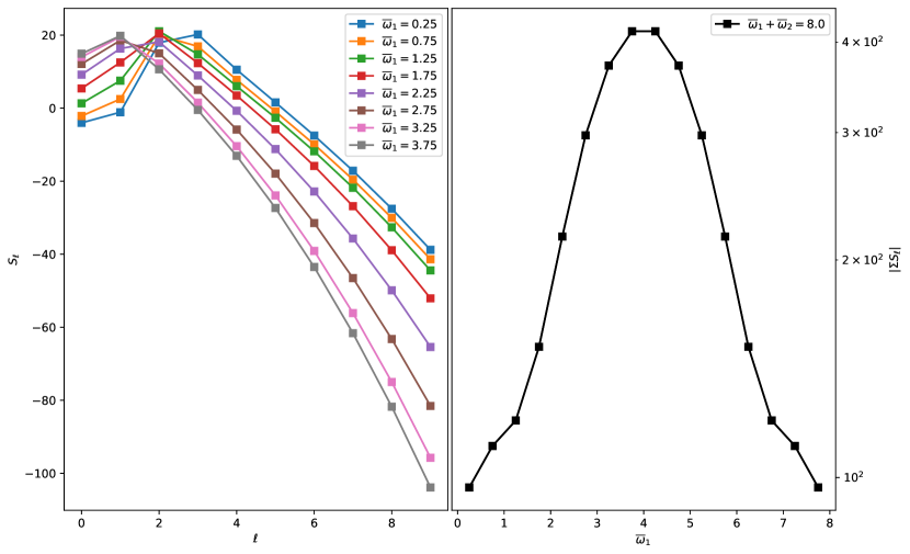
Refer to caption — Figure 1: Left: Evaluating (3.1) when $m^{2}=0$ for various choices of $\overline{\omega}$ . Right: The behaviour of $S_{\ell}$ for $\overline{\omega}$ values near $\omega_{0}$ .

In figures 1 and 2, we evaluate (3.1) for $\ell<10$ over a variety of $\overline{\omega}$ values first for a massless scalar, then for a tachyonic scalar. For both values of mass-squared, $\overline{T}_{\ell}$ demonstrates power law-type behaviour as a function of $\ell$ with a leading coefficient that is proportional to the non-normalizable frequency $\overline{\omega}$ . We also see that the limit of (3.1) as $\overline{\omega}\to\omega_{0}$ is well-defined in both cases.

3.2 Special Values of Non-normalizable Frequencies

Let us now consider special values of non-normalizable frequencies that will lead to a greater number of resonance channels. While general non-normalizable frequencies do not require any such restrictions, we will find it informative to examine these special cases as they possess more symmetry in index/frequency values than the case of equal non-normalizable frequencies, but less than all-normalizable modes.

3.2.1 Add to an integer

First, we choose the driving term to be given by the sum of two terms whose frequencies $\overline{\omega}_{1}$ and $\overline{\omega}_{2}$ add to give an integer

\displaystyle\mathcal{F}(t)=\bar{A}_{1}\cos\overline{\omega}_{1}t+\bar{A}_{2}\cos\overline{\omega}_{2}t\,,

(38)

where $\overline{\omega}_{1}+\overline{\omega}_{2}=2n$ and $n=1,2,3,\ldots$ (note that the $n=0$ case means that both $\overline{\omega}_{1}$ and $\overline{\omega}_{2}$ would need to be zero by the positive-frequency requirement and so would not contribute). Once again, the amplitudes $\bar{A}_{1}$ and $\bar{A}_{2}$ are constant and fixed by the form of $\mathcal{F}(t)$ . Furthermore, since neither frequency is restricted to integer values, the difference $|\overline{\omega}_{1}-\overline{\omega}_{2}|$ will, in general, not be an integer. In § 3.3, we examine the case when the difference of non-normalizable frequencies is an integer.

When we consider possible resonance channels, we find two resonances are present for any mass value within $m^{2}_{BF}<m^{2}\leq 0$ ,

	$\displaystyle(++):\;\omega_{i}+2n$	$\displaystyle=\omega_{\ell}\quad\forall\;\ell\geq n$		(39)
	$\displaystyle(+-):\,\omega_{i}-2n$	$\displaystyle=\omega_{\ell}\quad\forall\;n\,,$		(40)

while one channel is restricted to massless scalars¹¹1Note that specific values of $m^{2}\neq 0$ are capable of producing this kind of resonance channel. In such a case, the condition in (41) would be $n\geq\ell+\Delta^{+}$ with $m$ , $d$ such that $\Delta^{+}\in\;\mathbb{Z}^{+}$ .

\displaystyle(-+):\,-\omega_{i}+2n=\omega_{\ell}\quad\forall\;n\geq\ell+d\,.

(41)

Furthermore, for all allowed values of $n$ and $m^{2}$ , there are extra contributions due to resonances of the form of (34), i.e.

\displaystyle\omega_{i}+\overline{\omega}_{1}-\overline{\omega}_{1}=\omega_{i}+\overline{\omega}_{2}-\overline{\omega}_{2}=\omega_{\ell}\quad\forall\;n\,.

(42)

Adding the channels together, the total source term is

$\displaystyle S_{\ell}$	$\displaystyle=\!\!\!\!\sum_{\overline{\omega}_{1}+\overline{\omega}_{2}=2n}\bigg{[}\Theta\left(n-\ell-d\right)\overline{R}^{(-+)}_{(n-\ell-d)\ell}\ \bar{A}_{1}\bar{A}_{2}\,a_{(n-\ell-d)}\cos\left(\theta_{(n-\ell-d)}-\theta_{1}-\theta_{2}\right)\bigg{]}_{m^{2}=0}$
	$\displaystyle\quad+\!\!\!\!\sum_{\overline{\omega}_{1}+\overline{\omega}_{2}=2n}\!\!\!\!\Theta\left(\ell-n\right)\overline{R}^{(++)}_{(\ell-n)\ell}\,\bar{A}_{1}\bar{A}_{2}\,a_{(\ell-n)}\cos\left(\theta_{(\ell-n)}+\theta_{1}+\theta_{2}\right)$
	$\displaystyle\quad+\!\!\!\!\sum_{\overline{\omega}_{1}+\overline{\omega}_{2}=2n}\!\!\!\!\overline{R}^{(+-)}_{(\ell+n)\ell}\,\bar{A}_{1}\bar{A}_{2}\,a_{(\ell+n)}\cos\left(\theta_{(\ell+n)}-\theta_{1}-\theta_{2}\right)$
	$\displaystyle\quad+\!\!\!\!\sum_{\overline{\omega}_{1}+\overline{\omega}_{2}=2n}\!\!\!\!\overline{U}^{(1)}_{(\ell)\ell}\,\bar{A}_{1}^{2}\,a_{\ell}\cos\left(\theta_{(\ell)}+\theta_{1}-\theta_{1}\right)+\!\!\!\!\sum_{\overline{\omega}_{1}+\overline{\omega}_{2}=2n}\!\!\!\!\overline{U}^{(2)}_{(\ell)\ell}\,\bar{A}_{2}^{2}\,a_{\ell}\cos\left(\theta_{(\ell)}+\theta_{2}-\theta_{2}\right)$
	$\displaystyle\quad+\!\!\!\!\sum_{\overline{\omega}_{1}+\overline{\omega}_{2}=2n}\!\!\!\!\overline{T}^{(1)}_{\ell}\bar{A}_{1}^{2}\,a_{\ell}\cos\left(\theta_{\ell}\right)+\!\!\!\!\sum_{\overline{\omega}_{1}+\overline{\omega}_{2}=2n}\!\!\!\!\overline{T}^{(2)}_{\ell}\bar{A}_{2}^{2}\,a_{\ell}\cos\left(\theta_{\ell}\right)$	(43)

where the Heaviside step function $\Theta(x)$ enforces the restrictions on the indices in (39) and (41) and $\theta_{1}=\overline{\omega}_{1}t+\bar{B}_{1}$ , etc.

In the following expressions, the sum over all $\overline{\omega}_{1}$ , $\overline{\omega}_{2}$ such that $\overline{\omega}_{1}+\overline{\omega}_{2}=2n$ is implied, and only the restrictions on individual frequencies are included. Examining each channel in (3.2.1) individually, we find

$\displaystyle\overline{R}^{(++)}_{i\ell}$	$\displaystyle=-\frac{1}{4}\sum_{\overline{\omega}_{2}\neq\omega_{\ell}}\frac{\overline{\omega}_{2}}{\omega_{\ell}-\overline{\omega}_{2}}Z^{-}_{i12\ell}-\frac{1}{4}\sum_{\overline{\omega}_{1}\neq\omega_{\ell}}\frac{\overline{\omega}_{1}}{\omega_{\ell}-\overline{\omega}_{1}}Z^{-}_{i21\ell}-\frac{1}{8n}\left(\omega_{\ell}-2n\right)Z^{-}_{12i\ell}$
	$\displaystyle-\frac{1}{4}\sum_{\omega_{i}\neq\overline{\omega}_{1}}\frac{1}{\omega_{\ell}-\overline{\omega}_{2}}\Big{[}\overline{\omega}_{1}\left(H_{i12\ell}+m^{2}V_{12i\ell}-2\overline{\omega}_{2}^{2}X_{i12\ell}\right)+(\omega_{\ell}-2n)\left(H_{1i2\ell}+m^{2}V_{i21\ell}-2\overline{\omega}_{2}^{2}X_{1i2\ell}\right)\Big{]}$
	$\displaystyle-\frac{1}{4}\sum_{\omega_{i}\neq\overline{\omega}_{2}}\frac{1}{\omega_{\ell}-\overline{\omega}_{1}}\Big{[}\overline{\omega}_{2}\left(H_{i21\ell}+m^{2}V_{21i\ell}-2\overline{\omega}_{1}^{2}X_{i21\ell}\right)+(\omega_{\ell}-2n)\left(H_{2i1\ell}+m^{2}V_{i12\ell}-2\overline{\omega}_{1}^{2}X_{2i1\ell}\right)\Big{]}$
	$\displaystyle-\frac{1}{8n}\sum_{\overline{\omega}_{1}\neq\overline{\omega}_{2}}\Big{[}\overline{\omega}_{1}H_{21i\ell}+\overline{\omega}_{2}H_{12i\ell}+m^{2}\left(\overline{\omega}_{1}V_{1i2\ell}+\overline{\omega}_{2}V_{2i1\ell}\right)-\left(\omega_{\ell}-2n\right)^{2}\left(\overline{\omega}_{1}X_{21i\ell}+\overline{\omega}_{2}X_{12i\ell}\right)\Big{]}$
	$\displaystyle+\frac{1}{2}\Big{[}\overline{\omega}_{1}\overline{\omega}_{2}X_{i12\ell}+\left(\omega_{\ell}-2n\right)\left(\overline{\omega}_{1}X_{21i\ell}+\overline{\omega}_{2}X_{12i\ell}\right)-\frac{m^{2}}{2}\left(V_{i12\ell}+V_{i21\ell}+V_{12i\ell}\right)\Big{]}\,.$	(44)

The notation $X_{i12\ell}$ corresponds to evaluating $X_{ijk\ell}$ with $\omega_{j}=\overline{\omega}_{1}$ and $\omega_{k}=\overline{\omega}_{2}$ . Next, we find that

$\displaystyle\overline{R}_{i\ell}^{(+-)}$	$\displaystyle=-\frac{1}{4}\Big{[}\frac{(\omega_{\ell}+2n)}{2n}Z^{-}_{12i\ell}+2(\omega_{\ell}+2n)\left(\overline{\omega}_{1}X_{21i\ell}+\overline{\omega}_{2}X_{12i\ell}\right)$
	$\displaystyle-\frac{\overline{\omega}_{1}}{(\omega_{\ell}+\overline{\omega}_{2})}\left(H_{i12\ell}+m^{2}V_{12i\ell}-2\overline{\omega}_{2}^{2}X_{i12\ell}\right)+\frac{(\omega_{\ell}+2n)}{(\omega_{\ell}+\overline{\omega}_{2})}\left(H_{1i2\ell}+m^{2}V_{i21\ell}-2\overline{\omega}_{2}^{2}X_{1i2\ell}\right)$
	$\displaystyle-\frac{\overline{\omega}_{2}}{(\omega_{\ell}+\overline{\omega}_{1})}\left(H_{i21\ell}+m^{2}V_{21i\ell}-2\overline{\omega}_{1}^{2}X_{i21\ell}\right)+\frac{(\omega_{\ell}+2n)}{(\omega_{\ell}+\overline{\omega}_{1})}\left(H_{2i1\ell}+m^{2}V_{i12\ell}-2\overline{\omega}_{1}^{2}X_{2i1\ell}\right)$
	$\displaystyle-2\overline{\omega}_{1}\overline{\omega}_{2}X_{i12\ell}+m^{2}\left(V_{12i\ell}+V_{i12\ell}+V_{i21\ell}\right)\Big{]}+\frac{1}{4}\sum_{\overline{\omega}_{2}\neq\omega_{\ell}}\frac{\overline{\omega}_{1}\overline{\omega}_{2}(\omega_{\ell}+2n)}{\omega_{\ell}+\overline{\omega}_{2}}\left(X_{21i\ell}-X_{\ell i12}\right)$
	$\displaystyle+\frac{1}{4}\sum_{\overline{\omega}_{1}\neq\omega_{\ell}}\frac{\overline{\omega}_{1}\overline{\omega}_{2}(\omega_{\ell}+2n)}{\omega_{\ell}+\overline{\omega}_{1}}\left(X_{12i\ell}-X_{\ell i12}\right).$	(45)

When $m^{2}=0$ , we have contributions from

$\displaystyle\overline{R}_{i\ell}^{(-+)}$	$\displaystyle=\frac{1}{4}\sum_{\overline{\omega}_{2}\neq\omega_{\ell}}\frac{\overline{\omega}_{2}}{\omega_{\ell}-\overline{\omega}_{2}}Z^{+}_{i12\ell}+\frac{1}{4}\sum_{\overline{\omega}_{1}\neq\omega_{\ell}}\frac{\overline{\omega}_{1}}{\omega_{\ell}-\overline{\omega}_{1}}Z^{+}_{i21\ell}+\frac{1}{4}\sum_{i\neq\ell}\left(\frac{2n-\omega_{\ell}}{2n}\right)Z^{-}_{12i\ell}$
	$\displaystyle\quad+\frac{1}{4}\sum_{\overline{\omega}_{1}\neq\omega_{i}}\frac{1}{\omega_{i}-\overline{\omega}_{1}}\Big{[}\overline{\omega}_{1}\left(H_{i12\ell}-2\overline{\omega}_{2}^{2}X_{i12\ell}\right)-(2n-\omega_{\ell})\left(H_{1i2\ell}-2\overline{\omega}_{2}^{2}X_{1i2\ell}\right)\Big{]}$
	$\displaystyle\quad+\frac{1}{4}\sum_{\overline{\omega}_{2}\neq\omega_{i}}\frac{1}{\omega_{i}-\overline{\omega}_{2}}\Big{[}\overline{\omega}_{2}\left(H_{i21\ell}-2\overline{\omega}_{1}^{2}X_{i21\ell}\right)-(2n-\omega_{\ell})\left(H_{2i1\ell}-2\overline{\omega}_{1}^{2}X_{2i1\ell}\right)\Big{]}$
	$\displaystyle\quad-\frac{1}{8n}\sum_{\overline{\omega}_{1}\neq\overline{\omega}_{2}}\Big{[}\overline{\omega}_{1}H_{21i\ell}+\overline{\omega}_{2}H_{12i\ell}-2\left(2n-\omega_{\ell}\right)^{2}\left(\overline{\omega}_{1}X_{21i\ell}+\overline{\omega}_{2}X_{12i\ell}\right)\Big{]}$
	$\displaystyle\quad-\frac{1}{2}\Big{[}(2n-\omega_{\ell})\left(\overline{\omega}_{1}X_{21i\ell}+\overline{\omega}_{2}X_{12i\ell}\right)-\overline{\omega}_{1}\overline{\omega}_{2}X_{i12\ell}\Big{]}.$	(46)

NB. In (3.2.1) only, $\omega_{i}=2i+\Delta^{+}=2i+d$ since this term requires that $m^{2}=0$ to contribute. We maintain the same notation out of convenience, despite the special case. Finally,

	$\displaystyle\overline{U}^{(1)}_{i\ell}$	$\displaystyle=\sum_{\omega_{i}\neq\overline{\omega}_{1}}\left[\frac{\overline{\omega}_{1}^{2}}{\omega_{i}^{2}-\overline{\omega}_{1}^{2}}\left(H_{i11\ell}+m^{2}V_{11i\ell}-2\overline{\omega}_{1}^{2}X_{i11\ell}\right)-\frac{\omega_{i}^{2}}{\omega_{i}^{2}-\overline{\omega}_{1}^{2}}\left(H_{1i1\ell}+m^{2}V_{i11\ell}-2\overline{\omega}_{1}^{2}X_{11i\ell}\right)\right]$
		$\displaystyle\!\!\!\!+\frac{1}{2}\sum_{\omega_{\ell}\neq\overline{\omega}_{1}}\left[\frac{\overline{\omega}_{1}}{\omega_{\ell}+\overline{\omega}_{1}}Z^{-}_{i11\ell}+\frac{\overline{\omega}_{1}}{\omega_{\ell}-\overline{\omega}_{1}}Z^{+}_{i11\ell}\right]+\frac{1}{2}\omega_{\ell}^{2}\tilde{Z}^{+}_{11\ell}-\overline{\omega}_{1}^{2}X_{i11\ell}-\frac{1}{2}m^{2}V_{i11\ell}\,,$		(47)

and

\displaystyle\overline{T}^{(1)}_{\ell}=-\frac{1}{2}\left[H_{11\ell\ell}+m^{2}V_{\ell 11\ell}-2\omega_{\ell}^{2}X_{11\ell\ell}+4\omega_{\ell}^{2}\overline{\omega}_{1}^{2}P_{\ell\ell 1}+2\overline{\omega}_{1}^{2}M_{\ell\ell 1}+2m^{2}\overline{\omega}_{1}^{2}Q_{\ell\ell 1}\right]\,.

(48)

Where $\overline{U}^{(2)}_{i\ell}$ and $\overline{T}^{(2)}_{\ell}$ follow from (3.2.1) and (48) by replacing $\overline{\omega}_{1}\to\overline{\omega}_{2}$ .

In figure 3, we compute the total source term (modulo the amplitudes $a_{i}$ and $\bar{A}_{\alpha}$ ) for a tachyonic scalar with $n=2$ . Figure 4 provides a comparison between the value of the source term for a massless scalar between two choices of $n$ : one that includes contributions from $\overline{R}_{i\ell}^{(-+)}$ and one that does not. As expected, the source terms are symmetric in $\overline{\omega}_{1}\leftrightarrow\overline{\omega}_{2}$ , hence only $\overline{\omega}_{1}\leq n$ data are shown. Evaluations of each channel separately found that none vanished naturally. Since the total source term $S_{\ell}$ given by (3.2.1) initially evaluates to small, positive values before becoming increasingly negative as $\ell$ becomes large, one may ask if the sum of the channels vanishes. As a check for this, the absolute value of the sum of $S_{\ell}$ is also plotted; however, there is no indication that any channel vanishes for any of the $\overline{\omega}_{1}$ , $\overline{\omega}_{2}$ values considered.

The renormalization flow equations include the sum of all the channels (none of which vanish naturally), and are

$\displaystyle\frac{2\omega_{\ell}}{\epsilon^{2}}\frac{da_{\ell}}{dt}$	$\displaystyle=-\!\!\!\!\sum_{\overline{\omega}_{1}+\overline{\omega}_{2}=2n}\bigg{[}\Theta\left(n-\ell-d\right)\overline{R}^{(-+)}_{(n-\ell-d)\ell}\ \bar{A}_{1}\bar{A}_{2}\,a_{(n-\ell-d)}\sin\left(b_{(n-\ell-d)}-\bar{B}_{1}-\bar{B}_{2}\right)\bigg{]}_{m^{2}=0}$
	$\displaystyle\quad-\!\!\!\!\sum_{\overline{\omega}_{1}+\overline{\omega}_{2}=2n}\!\!\!\!\Theta\left(\ell-n\right)\overline{R}^{(++)}_{(\ell-n)\ell}\,\bar{A}_{1}\bar{A}_{2}\,a_{(\ell-n)}\sin\left(b_{(\ell-n)}+\bar{B}_{1}+\bar{B}_{2}\right)$
	$\displaystyle\quad-\!\!\!\!\sum_{\overline{\omega}_{1}+\overline{\omega}_{2}=2n}\!\!\!\!\overline{R}^{(+-)}_{(\ell+n)\ell}\,\bar{A}_{1}\bar{A}_{2}\,a_{(\ell+n)}\sin\left(b_{(\ell+n)}-\bar{B}_{1}-\bar{B}_{2}\right)\,,$	(49)

and

$\displaystyle\frac{2\omega_{\ell}a_{\ell}}{\epsilon^{2}}\frac{db_{\ell}}{dt}$	$\displaystyle=-\!\!\!\!\sum_{\overline{\omega}_{1}+\overline{\omega}_{2}=2n}\bigg{[}\Theta\left(n-\ell-d\right)\overline{R}^{(-+)}_{(n-\ell-d)\ell}\ \bar{A}_{1}\bar{A}_{2}\,a_{(n-\ell-d)}\cos\left(b_{(n-\ell-d)}-\bar{B}_{1}-\bar{B}_{2}\right)\bigg{]}_{m^{2}=0}$
	$\displaystyle\quad-\!\!\!\!\sum_{\overline{\omega}_{1}+\overline{\omega}_{2}=2n}\!\!\!\!\Theta\left(\ell-n\right)\overline{R}^{(++)}_{(\ell-n)\ell}\,\bar{A}_{1}\bar{A}_{2}\,a_{(\ell-n)}\cos\left(b_{(\ell-n)}+\bar{B}_{1}+\bar{B}_{2}\right)$
	$\displaystyle\quad-\!\!\!\!\sum_{\overline{\omega}_{1}+\overline{\omega}_{2}=2n}\!\!\!\!\overline{R}^{(+-)}_{(\ell+n)\ell}\,\bar{A}_{1}\bar{A}_{2}\,a_{(\ell+n)}\cos\left(b_{(\ell+n)}-\bar{B}_{1}-\bar{B}_{2}\right)$
	$\displaystyle\quad-\!\!\!\!\sum_{\overline{\omega}_{1}+\overline{\omega}_{2}=2n}\!\!\!\!a_{\ell}\left(\bar{A}_{1}^{2}(\overline{U}^{(1)}_{(\ell)\ell}+\overline{T}^{(1)}_{\ell})+\bar{A}_{2}^{2}(\overline{U}^{(2)}_{(\ell)\ell}+\overline{T}^{(2)}_{\ell})\right)\,.$	(50)

3.3 Integer Plus $\chi$

Finally, let us consider the case where the boundary condition can be written in terms of a sum of non-normalizable modes with constant amplitudes $\bar{A}_{\gamma}$ and frequencies $\omega_{\gamma}$ that are each non-integer valued, but differ from integer values by a set amount, i.e.

\displaystyle\mathcal{F}(t)=\sum_{\gamma}\bar{A}_{\gamma}\cos\left(\omega_{\gamma}t+\bar{B}_{\gamma}\right)\quad\text{with}\quad\omega_{\gamma}=2\gamma+\chi\,,

(51)

where $\gamma\in\mathbb{Z}^{+}$ . Greek letters are chosen to differentiate these non-normalizable modes from normalizable modes with integer frequencies, which use Roman letters. We furthermore limit $\chi$ to be non-integer²²2Indeed, for integer values of $\chi$ , the sum or difference of two non-normalizable modes could be an integer. This would either be covered by the work in § 3.2.1, or be a slight variation of it. and set $m^{2}=0$ throughout. For this choice of non-normalizable frequencies there are no resonant contributions from the all-plus channel, unlike the naturally vanishing resonance found in § C.1. Only when either $\omega_{i}+\omega_{\gamma}=\omega_{\beta}-\omega_{\ell}$ , or $\omega_{i}+\omega_{\gamma}=\omega_{\beta}+\omega_{\ell}$ with $i+\gamma\geq\ell$ , are resonant terms present. Let us examine each case separately.

3.3.1 $\omega_{i}+\omega_{\gamma}=\omega_{\beta}-\omega_{\ell}$

The resonance condition $\omega_{i}+\omega_{\gamma}=\omega_{\beta}-\omega_{\ell}$ will contribute two types of terms to $S_{\ell}$ . The first term includes a double sum over the frequencies $\omega_{i}$ and $\omega_{\gamma}$ with $\beta=i+\gamma+\ell$ and $\beta\neq\gamma$ , and the second term includes a single sum over $\omega_{\gamma}$ with $\beta=\gamma+2\ell+d$ . In total, the source term is of the form

	$\displaystyle S_{\ell}$	$\displaystyle=\sum_{i\neq\ell}\sum_{\gamma\neq\beta}\overline{S}^{(1)}_{i(i+\gamma+\ell)\gamma\ell}\,a_{i}\bar{A}_{(i+\gamma+\ell)}\bar{A}_{\gamma}\cos\left(\theta_{i}-\theta_{(i+\gamma+\ell)}+\theta_{\gamma}\right)$
		$\displaystyle\qquad+\sum_{\gamma}\overline{R}^{(1)}_{(\gamma+2\ell+d)\ell}\,a_{\ell}\bar{A}_{\gamma}\bar{A}_{(\gamma+2\ell+d)}\cos\left(\theta_{\ell}-\theta_{(\gamma+2\ell+d)}+\theta_{\gamma}\right)\,,$		(52)

where

$\displaystyle\overline{S}^{(1)}_{i\beta\gamma\ell}$	$\displaystyle=\frac{1}{4}H_{\beta\gamma i\ell}\frac{\omega_{\gamma}(\omega_{i}-\omega_{\beta}+2\omega_{\gamma})}{(\omega_{\beta}-\omega_{\gamma})(\omega_{i}+\omega_{\gamma})}-\frac{1}{4}H_{\gamma\beta i\ell}\frac{\omega_{\beta}(\omega_{i}+\omega_{\gamma}-2\omega_{\beta})}{(\omega_{i}-\omega_{\beta})(\omega_{\beta}-\omega_{\gamma})}-\frac{1}{4}H_{\gamma i\beta\ell}\frac{\omega_{i}(\omega_{\gamma}-\omega_{\beta}+2\omega_{i})}{(\omega_{i}-\omega_{\beta})(\omega_{i}+\omega_{\gamma})}$
	$\displaystyle+\frac{1}{2}\omega_{i}\omega_{\gamma}X_{\beta\gamma i\ell}\left(\frac{\omega_{\gamma}}{\omega_{i}-\omega_{\beta}}-\frac{\omega_{i}}{\omega_{\beta}+\omega_{\gamma}}+1\right)+\frac{1}{2}\omega_{i}\omega_{\beta}X_{\gamma\beta i\ell}\left(\frac{\omega_{i}}{\omega_{\beta}-\omega_{\gamma}}+\frac{\omega_{\beta}}{\omega_{i}+\omega_{\gamma}}-1\right)$
	$\displaystyle+\frac{1}{2}\omega_{\beta}\omega_{\gamma}X_{i\beta\gamma\ell}\left(\frac{\omega_{\beta}}{\omega_{i}+\omega_{\gamma}}-\frac{\omega_{\gamma}}{\omega_{i}-\omega_{\beta}}-1\right)-\frac{1}{4}Z^{+}_{\beta\gamma i\ell}\left(\frac{\omega_{i}}{\omega_{i}+\omega_{\ell}}\right)$
	$\displaystyle+\frac{1}{4}Z^{-}_{i\gamma\beta\ell}\left(\frac{\omega_{\beta}}{\omega_{\ell}-\omega_{\beta}}\right)+\frac{1}{4}Z^{+}_{i\beta\gamma\ell}\left(\frac{\omega_{\gamma}}{\omega_{\ell}+\omega_{\gamma}}\right)\,,$	(53)

and

$\displaystyle\overline{R}^{(1)}_{\beta\ell}$	$\displaystyle=-\frac{1}{4}Z^{-}_{\gamma\ell\beta\ell}\left(\frac{\omega_{\beta}}{\omega_{\ell}-\omega_{\beta}}\right)-\frac{1}{4}Z^{+}_{\ell\beta\gamma\ell}\left(\frac{\omega_{\gamma}}{\omega_{\ell}+\omega_{\gamma}}\right)+\frac{1}{8}H_{\beta\gamma\ell\ell}\frac{\omega_{\gamma}(\omega_{\gamma}-\omega_{\ell})}{\omega_{\ell}(\omega_{\ell}+\omega_{\gamma})}+\frac{1}{8}H_{\gamma\beta\ell\ell}\frac{\omega_{\beta}(\omega_{\ell}-\omega_{\gamma})}{\omega_{\ell}(\omega_{\ell}+\omega_{\gamma})}$
	$\displaystyle-\frac{1}{4}\omega_{\gamma}\omega_{\ell}X_{\beta\gamma\ell\ell}\frac{(\omega_{\ell}-\omega_{\gamma})}{(\omega_{\ell}+\omega_{\gamma})}+\frac{1}{4}\omega_{\beta}\omega_{\ell}X_{\gamma\beta\ell\ell}\frac{(\omega_{\ell}+\omega_{\gamma}+2\omega_{\beta})}{(\omega_{\ell}+\omega_{\gamma})}+\frac{1}{2}\omega_{\beta}\omega_{\gamma}X_{\ell\ell\beta\gamma}\frac{(\omega_{\gamma}+\omega_{\beta})}{(\omega_{\ell}+\omega_{\gamma})}$
	$\displaystyle-\frac{1}{2}\omega_{\ell}\omega_{\beta}X_{\gamma\beta\ell\ell}-\frac{1}{2}\omega_{\beta}\omega_{\gamma}X_{\ell\ell\beta\gamma}+\frac{1}{2}\omega_{\ell}\omega_{\gamma}X_{\beta\gamma\ell\ell}-\omega_{\ell}^{2}\tilde{Z}^{+}_{\beta\gamma\ell}\,.$	(54)

3.3.2 $\omega_{i}+\omega_{\gamma}=\omega_{\beta}+\omega_{\ell}$

Similarly, when the resonance condition $\omega_{i}+\omega_{\gamma}=\omega_{\beta}+\omega_{\ell}$ is met, the contribution to the source term is

	$\displaystyle S_{\ell}$	$\displaystyle=\underbrace{\sum_{i\neq\ell}\sum_{\gamma\neq\beta}}_{i+\gamma\geq\ell}\overline{S}^{(2)}_{i(i+\gamma-\ell)\gamma\ell}\,a_{i}\bar{A}_{(i+\gamma-\ell)}\bar{A}_{\gamma}\cos\left(\theta_{i}-\theta_{(i+\gamma-\ell)}+\theta_{\gamma}\right)$
		$\displaystyle\qquad\qquad+\sum_{\beta}\overline{R}^{(2)}_{\beta\ell}\,a_{\ell}\bar{A}_{\beta}^{2}\cos\left(\theta_{\ell}+\theta_{\beta}-\theta_{\beta}\right)\,,$		(55)

where

$\displaystyle\overline{S}^{(2)}_{i\beta\gamma\ell}$	$\displaystyle=\frac{1}{4}H_{\beta\gamma i\ell}\frac{\omega_{\gamma}(\omega_{i}-\omega_{\beta})}{(\omega_{\beta}-\omega_{\gamma})(\omega_{i}-\omega_{\gamma})}-\frac{1}{4}H_{\gamma\beta i\ell}\frac{\omega_{\beta}(\omega_{\ell}-\omega_{\beta})}{(\omega_{\beta}-\omega_{\gamma})(\omega_{i}-\omega_{\beta})}+\frac{1}{4}H_{\beta i\gamma\ell}\frac{\omega_{i}(\omega_{\gamma}-\omega_{\beta})}{(\omega_{i}-\omega_{\beta})(\omega_{i}-\omega_{\gamma})}$
	$\displaystyle+\frac{1}{2}\omega_{i}\omega_{\gamma}X_{\beta\gamma i\ell}\left(\frac{\omega_{\gamma}}{\omega_{i}-\omega_{\beta}}-\frac{\omega_{i}}{\omega_{\beta}-\omega_{\gamma}}+1\right)+\frac{1}{2}\omega_{i}\omega_{\beta}X_{\gamma\beta i\ell}\left(\frac{\omega_{i}}{\omega_{\beta}-\omega_{\gamma}}-\frac{\omega_{\beta}}{\omega_{i}-\omega_{\gamma}}-1\right)$
	$\displaystyle+\frac{1}{2}\omega_{\beta}\omega_{\gamma}X_{i\beta\gamma\ell}\left(\frac{\omega_{\beta}}{\omega_{i}-\omega_{\gamma}}-\frac{\omega_{\gamma}}{\omega_{i}-\omega_{\beta}}-1\right)+\frac{1}{4}Z^{-}_{i\gamma\beta\ell}\left(\frac{\omega_{\beta}}{\omega_{\ell}+\omega_{\beta}}\right)$
	$\displaystyle+\frac{1}{4}Z^{+}_{i\beta\gamma\ell}\left(\frac{\omega_{\gamma}}{\omega_{\ell}-\omega_{\gamma}}\right)-\frac{1}{4}Z^{+}_{\beta\gamma i\ell}\left(\frac{\omega_{i}}{\omega_{i}-\omega_{\ell}}\right)\,,$	(56)

and

	$\displaystyle\overline{R}^{(2)}_{\beta\ell}$	$\displaystyle=\frac{1}{4}Z^{-}_{\ell\beta\beta\ell}\left(\frac{\omega_{\beta}}{\omega_{\ell}+\omega_{\beta}}\right)+\frac{1}{4}Z^{+}_{\ell\beta\beta\ell}\left(\frac{\omega_{\beta}}{\omega_{\ell}-\omega_{\beta}}\right)+\frac{1}{2}H_{\ell\beta\beta\ell}\left(\frac{\omega_{\beta}^{2}}{\omega_{\ell}^{2}-\omega_{\beta}^{2}}\right)-\frac{1}{2}H_{\beta\ell\beta\ell}\left(\frac{\omega_{\ell}^{2}}{\omega_{\ell}^{2}-\omega_{\beta}^{2}}\right)$
		$\displaystyle\!\!\!\!\!\!\!\!+X_{\beta\beta\ell\ell}\left(\frac{\omega_{\ell}^{2}}{\omega_{\ell}^{2}-\omega_{\beta}^{2}}\right)+\frac{1}{2}\omega_{\beta}^{2}X_{\ell\beta\beta\ell}\left(\frac{\omega_{\ell}^{2}+\omega_{\beta}^{2}}{\omega_{\ell}^{2}-\omega_{\beta}^{2}}\right)-\frac{1}{2}H_{\beta\beta\ell\ell}+\omega_{\ell}^{2}\tilde{Z}^{+}_{\beta\beta\ell}-2\omega_{\beta}^{2}\omega_{\ell}^{2}P_{\ell\ell\beta}-\omega_{\beta}^{2}M_{\ell\ell\beta}.\vspace{-0.3in}$		(57)

Unlike the case with all normalizable modes where two of the three resonance channels naturally vanished, both of the resonant channels contribute when the non-normalizable modes have frequencies given by (51). Therefore, the renormalization flow equations will contain contributions from both channels:

	$\displaystyle\frac{2\omega_{\ell}}{\epsilon^{2}}\frac{da_{\ell}}{dt}$	$\displaystyle=-\sum_{i\neq\ell}\sum_{\gamma\neq\beta}\overline{S}^{(1)}_{i(i+\gamma+\ell)\gamma\ell}\,a_{i}\bar{A}_{(i+\gamma+\ell)}\bar{A}_{\gamma}\sin\left(b_{\ell}+\bar{B}_{(i+\gamma+\ell)}-b_{i}-\bar{B}_{\gamma}\right)$
		$\displaystyle\qquad\qquad-\underbrace{\sum_{i\neq\ell}\sum_{\gamma\neq\beta}}_{i+\gamma\geq\ell}\overline{S}^{(2)}_{i(i+\gamma-\ell)\gamma\ell}\,a_{i}\bar{A}_{(i+\gamma-\ell)}\bar{A}_{\gamma}\sin\left(b_{\ell}+\bar{B}_{(i+\gamma-\ell)}-b_{i}-\bar{B}_{\gamma}\right)\,,$		(58)

$\displaystyle\frac{2\omega_{\ell}a_{\ell}}{\epsilon^{2}}\frac{db_{\ell}}{dt}$	$\displaystyle=-\sum_{\beta}\overline{R}^{(2)}_{\beta\ell}\,a_{\ell}\bar{A}_{\beta}^{2}-\sum_{\gamma}\overline{R}^{(1)}_{(\gamma+2\ell+d)\ell}\,a_{\ell}\bar{A}_{\gamma}\bar{A}_{(\gamma+2\ell+d)}\cos\left(b_{\ell}-\bar{B}_{(\gamma+2\ell+d)}+\bar{B}_{\gamma}\right)$
	$\displaystyle\qquad-\sum_{i\neq\ell}\sum_{\gamma\neq\beta}\overline{S}^{(1)}_{i(i+\gamma+\ell)\gamma\ell}\,a_{i}\bar{A}_{(i+\gamma+\ell)}\bar{A}_{\gamma}\cos\left(-b_{\ell}+\bar{B}_{(i+\gamma+\ell)}-b_{i}-\bar{B}_{\gamma}\right)$
	$\displaystyle\qquad\qquad-\underbrace{\sum_{i\neq\ell}\sum_{\gamma\neq\beta}}_{i+\gamma\geq\ell}\overline{S}^{(2)}_{i(i+\gamma-\ell)\gamma\ell}\,a_{i}\bar{A}_{(i+\gamma-\ell)}\bar{A}_{\gamma}\cos\left(b_{\ell}+\bar{B}_{(i+\gamma-\ell)}-b_{i}-\bar{B}_{\gamma}\right)\,.$	(59)

In figure 5, we evaluate both resonant contributions channels’ and plot their contributions for various values of $\chi$ . In particular, we examine the values $\chi\in\{\pi/6,\ldots,7\pi/6\}$ . Again, there is no indication of any channel vanishing naturally. Interestingly, both sources demonstrate anomalous behaviour when $\chi\sim 2$ for reasons that are not immediately clear. The source term (3.3.1) is generally more positive for larger $\chi$ except for $\chi=2\pi/3$ , which is translated negatively with respect to the source terms produced by other $\chi$ values. Again, when (3.3.2) is evaluated for $\chi=2\pi/3$ , the result differs significantly from other choices of $\chi$ : seemingly reflected through the $x$ axis with respect to other results. The significance of the choice $\chi=2\pi/3\sim d/2$ is possibly explained by the non-normalizable modes being nearly equal to the normalizable ones. In this event, $S_{\ell}$ would contain additional terms, such as those present in § C. The departure of the $\chi=2\pi/3$ data from other data sets is perhaps a signal of these missing resonances.

4 Discussion

We have seen that the inclusion of a time-dependent boundary term in the holographic dual of a quantum quench allows energy to enter the bulk spacetime through coupling with non-normalizable modes. The dynamics of the weakly turbulent energy cascades that trigger instability were captured by secular terms at third-order that could not be removed by frequency shifts alone. Using the Two-Time Formalism, we have determined the flow equations for the slowly varying amplitudes and phases that are tuned to cancel the secular terms at each instant.

Following our discussion at the end of § 2, we have limited the types of resonances we have considered to only those produced when the resonance condition ${\omega_{I}\pm\omega_{J}\pm\omega_{K}=\pm\omega_{\ell}}$ contains exactly two non-normalizable frequencies. As a result, the flow equations for the time-dependent amplitudes and phases of the normal modes are linear in the amplitude. When only normalizable modes are considered, these equations contain three powers of the amplitude 1403.6471 ; 1407.6273 . It is important to note that the resonances from only normalizable modes are still present (see appendix C for their explicit forms) and would also contribute to the non-normalizable resonances. Furthermore, we have restricted our choice of mass to within $m_{BF}^{2}<m^{2}\leq 0$ to avoid potential issues raised by renormalizability of the metric functions ${A(t,x),~{}\delta(t,x)}$ on the boundary of AdS. Future work will consider what counterterms are required to keep the CFT renormalizable outside of this restriction on the mass. What remains to be shown is if, for some judicious choice of time-dependent boundary term, the different types of resonances would destructively interfere and render the perturbative description naturally stable.

We have considered a set of broadly applicable choices for the form of the driving term $\mathcal{F}(t)$ that require little or no fine tuning to produce resonant contributions. When the driving term is given by a single, non-integer frequency component, there is a single resonant channel and the presence of non-normalizable modes affects only the flow of the phase. While both $a_{\ell}$ and $b_{\ell}$ will also receive terms due to all-normalizable resonances, the fact that this choice of driving term induces extra drift in the phase only is interesting. By considering more specialized forms of the driving term, additional resonance channels from non-normalizable modes are present. Unlike when only normalizable modes are considered, none of the channels are naturally vanishing. When the driving term is given by the superposition of two periodic functions with frequencies that add to an integer, the flow equations for $a_{\ell}$ and $b_{\ell}$ receive contributions from multiple terms that mix modes. For example, (3.2.1) shows that $da_{\ell}/dt$ can contain contributions proportional to $a_{(n-\ell-d)}$ , $a_{(\ell-n)}$ , and $a_{(\ell+n)}$ . Further mixing of modes is observed when the driving term is given by a Fourier sum over frequencies that differ from an integer by a set amount. In this case, the equations for $da_{\ell}/dt$ and $db_{\ell}/dt$ both receive contributions from mixed normalizable amplitudes and non-normalizable amplitudes, e.g. $da_{\ell}/dt$ contains terms proportional to both ${\bar{A}_{(i+\gamma+\ell)}}$ and ${\bar{A}_{(i+\gamma-\ell)}}$ . Unlike when only normalizable modes are considered, there were no naturally vanishing resonance channels for the frequencies considered.

With the renormalization flow equations established, future work will compare the perturbatively stable solutions found from the TTF theory to the behaviour of the fully numerical systems in the limit of weak driving 1712.07637 ; 1502.05726 . Comparisons to established numerical pumped solutions in the full theory may be instructive in understanding the space of stable and nearly-stable data. Indeed, this was the case with the TTF description of a collapsing scalar field subject static boundary conditions 1507.08261 . Furthermore, the development of a perturbative description for pumped scalars may aide in solving the fully nonlinear system by reducing computational overhead when the full system is known to be well described by the TTF. Beyond this time, numerical methods could switch to conventional, computationally-complex methods as the system approaches collapse.

Acknowledgements.

The author would like to thank A. R. Frey for their guidance and insight with this project. This work is supported by the Natural Sciences and Engineering Research Council of Canada’s Discovery Grant program.

Appendix A Derivation of Source Terms For Massive Scalars

The derivation of the general expression for the $\mathcal{O}(\epsilon^{3})$ source term for massive scalars closely follows the massless case, particularly if one chooses not to write out the explicit mass dependence as was done in 1810.04753 . However, since we have chosen to write our equations in a slightly different way – and in a different gauge – than previous authors, one may find it instructive to see the differences in the derivations. Below we have included the intermediate steps involved in deriving the third-order source term $S_{\ell}$ .

Continuing the expansion of the equations of motion in powers of $\epsilon$ , we see that the backreaction between the metric and the scalar field appears at second order in the perturbation,

\displaystyle A_{2}^{\prime}=-\mu\nu\left[(\dot{\phi}_{1})^{2}+(\phi_{1}^{\prime})^{2}+m^{2}\phi_{1}^{2}\sec^{2}x\right]+\nu^{\prime}A_{2}/\nu\,,

(60)

which can be directly integrated to give

\displaystyle A_{2}=-\nu\int^{x}_{0}dy\,\mu\left((\dot{\phi}_{1})^{2}+(\phi_{1}^{\prime})^{2}+m^{2}\phi_{1}^{2}\sec^{2}x\right)\,.

(61)

For convenience, we have also defined the functions

\displaystyle\mu(x)=\left(\tan x\right)^{d-1}\quad\text{and}\quad\nu(x)=(d-1)/\mu^{\prime}\,.

(62)

Similarly, the first non-trivial contribution to the lapse (in the boundary time gauge) is

\displaystyle\delta_{2}=\int^{\pi/2}_{x}dy\,\mu\nu\left((\dot{\phi}_{1})^{2}+(\phi_{1}^{\prime})^{2}\right)\,.

(63)

Projecting each of the terms in (19) individually onto the eigenbasis $\{e_{\ell}\}$ will involve evaluating inner products involving multiple integrals. To aide in evaluating these expressions, it is useful to derive several identities. First, from the equation for the scalar field’s time-dependent coefficients $c_{i}$ ,

\displaystyle\ddot{c}_{i}+\omega_{i}^{2}c_{i}=0\quad\Rightarrow\quad\partial_{t}\left(\dot{c}_{i}^{2}+\omega_{i}^{2}c_{i}^{2}\right)=\partial_{t}\mathbb{C}_{i}=0\,.

(64)

Next, from the definition of $\hat{L}$ ,

\displaystyle\hat{L}e_{j}=-\frac{1}{\mu}\left(\mu e^{\prime}_{j}\right)^{\prime}+m^{2}\sec^{2}xe_{j}\quad\Rightarrow\quad\left(\mu e^{\prime}_{j}\right)^{\prime}=\mu\left(m^{2}\sec^{2}x-\omega_{j}^{2}\right)e_{j}\,.

(65)

By considering the expression $\left(\mu e^{\prime}_{i}e_{j}\right)^{\prime}$ , we see that

\displaystyle\left(\mu e^{\prime}_{i}e_{j}\right)^{\prime}=\left(m^{2}\sec^{2}x-\omega_{i}^{2}\right)\mu e_{i}e_{j}+\mu e^{\prime}_{i}e^{\prime}_{j}\,,

(66)

which, after permuting $i,j$ and subtracting from above, gives

\displaystyle\frac{\left[\mu(e^{\prime}_{i}e_{j}\omega_{j}^{2}-e_{i}e^{\prime}_{j}\omega_{i}^{2})\right]^{\prime}}{(\omega_{j}^{2}-\omega_{i}^{2})}=\mu m^{2}\sec^{2}xe_{i}e_{j}+\mu e^{\prime}_{i}e^{\prime}_{j}\,.

(67)

Using these identities, we evaluate each of the inner products and find that

$\displaystyle\langle\delta_{2}\ddot{\phi}_{1},e_{\ell}\rangle$	$\displaystyle=-\sum_{i=0}^{\infty}\sum_{\begin{subarray}{c}j=0\\ k\neq\ell\end{subarray}}^{\infty}\sum_{k=0}^{\infty}\frac{\omega_{k}^{2}c_{k}}{\omega_{\ell}^{2}-\omega_{k}^{2}}\left[\dot{c}_{i}\dot{c}_{j}\left(X_{k\ell ij}-X_{\ell kij}\right)+c_{i}c_{j}\left(Y_{ij\ell k}-Y_{ijk\ell}\right)\right]$
	$\displaystyle\qquad-\sum_{i=0}^{\infty}\sum_{j=0}^{\infty}\omega_{\ell}^{2}c_{\ell}\left[\dot{c}_{i}\dot{c}_{j}P_{ij\ell}+c_{i}c_{j}B_{ij\ell}\right]\,,$	(68)
$\displaystyle\langle A_{2}\ddot{\phi}_{1},e_{\ell}\rangle$	$\displaystyle=2\sum_{i=0}^{\infty}\sum_{\begin{subarray}{c}j=0\\ i\neq j\end{subarray}}^{\infty}\sum_{k=0}^{\infty}\frac{\omega_{k}^{2}c_{k}}{\omega_{j}^{2}-\omega_{i}^{2}}X_{ijk\ell}\left(\dot{c}_{i}\dot{c}_{j}+\omega_{j}^{2}c_{i}c_{j}\right)$
	$\displaystyle\qquad+\sum_{i=0}^{\infty}\sum_{j=0}^{\infty}\omega_{j}^{2}c_{j}\left(\mathbb{C}_{i}P_{j\ell i}+c_{i}^{2}X_{iij\ell}\right)\,,$	(69)
$\displaystyle\langle\dot{\delta}_{2}\dot{\phi}_{1},e_{\ell}\rangle$	$\displaystyle=\sum_{i=0}^{\infty}\sum_{\begin{subarray}{c}j=0\\ k\neq\ell\end{subarray}}^{\infty}\sum_{k=0}^{\infty}\frac{\dot{c}_{k}}{\omega_{\ell}^{2}-\omega_{k}^{2}}\left[\partial_{t}\left(\dot{c}_{i}\dot{c}_{j}\right)\left(X_{k\ell ij}-X_{\ell kij}\right)+\partial_{t}(c_{i}c_{j})\left(Y_{ij\ell k}-Y_{ijk\ell}\right)\right]$
	$\displaystyle\qquad+\sum_{i=0}^{\infty}\sum_{j=0}^{\infty}\dot{c}_{\ell}\left[\partial_{t}\left(\dot{c}_{i}\dot{c}_{j}\right)P_{ij\ell}+\partial_{t}(c_{i}c_{j})B_{ij\ell}\right]\,,$	(70)
$\displaystyle\langle\dot{A}_{2}\dot{\phi}_{1},e_{\ell}\rangle$	$\displaystyle=-2\sum_{i=0}^{\infty}\sum_{j=0}^{\infty}\sum_{k=0}^{\infty}\dot{c}_{k}\dot{c}_{j}c_{i}X_{ijk\ell}\,,$	(71)
$\displaystyle\langle\left(A_{2}^{\prime}-\delta_{2}^{\prime}\right)\phi_{1}^{\prime},e_{\ell}\rangle$	$\displaystyle=-2\sum_{i=0}^{\infty}\sum_{\begin{subarray}{c}j=0\\ i\neq j\end{subarray}}^{\infty}\sum_{k=0}^{\infty}\frac{c_{k}(\dot{c}_{i}\dot{c}_{j}+\omega_{j}^{2}c_{i}c_{j})}{\omega_{j}^{2}-\omega_{i}^{2}}H_{ijk\ell}-m^{2}\sum_{i=0}^{\infty}\sum_{j=0}^{\infty}\sum_{k=0}^{\infty}c_{i}c_{j}c_{k}V_{ijk\ell}$
	$\displaystyle\qquad-\sum_{i=0}^{\infty}\sum_{j=0}^{\infty}c_{j}\left[c_{i}^{2}H_{iij\ell}+\mathbb{C}_{i}M_{j\ell i}\right]\,,$	(72)
$\displaystyle\langle A_{2}\phi_{1}\sec^{2}x,e_{\ell}\rangle$	$\displaystyle=-2\sum_{i=0}^{\infty}\sum_{\begin{subarray}{c}j=0\\ i\neq j\end{subarray}}^{\infty}\sum_{k=0}^{\infty}\frac{c_{k}(\dot{c}_{i}\dot{c}_{j}+\omega_{j}^{2}c_{i}c_{j})}{\omega_{j}^{2}-\omega_{i}^{2}}V_{jki\ell}$
	$\displaystyle\qquad-\sum_{i=0}^{\infty}\sum_{j=0}^{\infty}c_{j}\left(c_{i}^{2}V_{jii\ell}+\mathbb{C}_{i}Q_{j\ell i}\right),$	(73)

where the forms of X, Y, V, H, B, M, P, and Q are given by

$\displaystyle X_{ijk\ell}$	$\displaystyle=\int^{\pi/2}_{0}dx\,\mu^{2}\nu e^{\prime}_{i}e_{j}e_{k}e_{\ell}$	(74)
$\displaystyle Y_{ijk\ell}$	$\displaystyle=\int^{\pi/2}_{0}dx\,\mu^{2}\nu e^{\prime}_{i}e^{\prime}_{j}e_{k}e^{\prime}_{\ell}$	(75)
$\displaystyle V_{ijk\ell}$	$\displaystyle=\int^{\pi/2}_{0}dx\,\mu^{2}\nu e_{i}e_{j}e^{\prime}_{k}e_{\ell}\sec^{2}x$	(76)
$\displaystyle H_{ijk\ell}$	$\displaystyle=\int^{\pi/2}_{0}dx\,\mu^{2}\nu^{\prime}e^{\prime}_{i}e_{j}e^{\prime}_{k}e_{\ell}$	(77)
$\displaystyle B_{ij\ell}$	$\displaystyle=\int^{\pi/2}_{0}dx\,\mu\nu e^{\prime}_{i}e^{\prime}_{j}\int^{x}_{0}dy\,\mu e^{2}_{\ell}$	(78)
$\displaystyle M_{ij\ell}$	$\displaystyle=\int^{\pi/2}_{0}dx\,\mu\nu^{\prime}e^{\prime}_{i}e_{j}\int^{x}_{o}dy\,\mu e_{\ell}^{2}$	(79)
$\displaystyle P_{ij\ell}$	$\displaystyle=\int^{\pi/2}_{0}dx\,\mu\nu e_{i}e_{j}\int^{x}_{0}dy\,\mu e^{2}_{\ell}$	(80)
$\displaystyle Q_{ij\ell}$	$\displaystyle=\int^{\pi/2}_{0}dx\,\mu\nu e_{i}e_{j}\sec^{2}x\int^{x}_{0}dy\,\mu e^{2}_{\ell}\,.$	(81)

Note that, using integration by parts to remove the derivative from $\nu$ in the definitions of $H_{ijk\ell}$ and $M_{ij\ell}$ , we can show that

	$\displaystyle H_{ijk\ell}$	$\displaystyle=\omega_{i}^{2}X_{kij\ell}+\omega_{k}^{2}X_{ijk\ell}-Y_{ij\ell k}-Y_{\ell kji}-m^{2}V_{kji\ell}-m^{2}V_{ijk\ell}\,,$		(82)
	$\displaystyle M_{ij\ell}$	$\displaystyle=\omega_{i}^{2}P_{ij\ell}-B_{ij\ell}-m^{2}Q_{ij\ell}\,.$		(83)

Collecting (A) - (A) gives the expression for $S_{\ell}=\langle S,e_{\ell}\rangle$ :

$\displaystyle S_{\ell}$	$\displaystyle=\sum_{\begin{subarray}{c}i,j,k\\ k\neq\ell\end{subarray}}^{\infty}\frac{1}{\omega_{\ell}^{2}-\omega_{k}^{2}}\Big{[}F_{k}(\dot{c}_{i}\dot{c}_{j})\left(X_{k\ell ij}-X_{\ell kij}\right)+F_{k}(c_{i}c_{j})\left(Y_{ij\ell k}-Y_{ijk\ell}\right)\Big{]}$
	$\displaystyle\quad+2\sum_{\begin{subarray}{c}i,j,k\\ i\neq j\end{subarray}}^{\infty}\frac{c_{k}D_{ij}}{\omega_{j}^{2}-\omega_{i}^{2}}\Big{[}2\omega_{k}^{2}X_{ijk\ell}-H_{ijk\ell}-m^{2}V_{jki\ell}\Big{]}-\sum_{i,j,k}^{\infty}c_{i}\Big{[}2\dot{c}_{j}\dot{c}_{k}X_{ijk\ell}+m^{2}c_{j}c_{k}V_{ijk\ell}\Big{]}$
	$\displaystyle\quad+\sum_{i,j}^{\infty}\Big{[}F_{\ell}(\dot{c}_{i}\dot{c}_{j})P_{ij\ell}+F_{\ell}(c_{i}c_{j})B_{ij\ell}+2\omega_{j}^{2}c_{j}\left(c_{i}^{2}X_{iij\ell}+\mathbb{C}_{i}P_{j\ell i}\right)$
	$\displaystyle\qquad-c_{j}\left(c^{2}_{i}(H_{iij\ell}+m^{2}V_{jii\ell})+\mathbb{C}_{i}(M_{j\ell i}+m^{2}Q_{j\ell i})\right)\Big{]}\,,$	(84)

where $F_{k}(z)=\dot{c}_{k}\dot{z}-2\omega_{k}^{2}c_{k}z$ , $D_{ij}=\dot{c}_{i}\dot{c}_{j}+\omega^{2}_{j}c_{i}c_{j}$ , and $\mathbb{C}_{i}=\dot{c}_{i}^{2}+\omega_{i}^{2}c_{i}^{2}$ . Additionally, we have combined some integrals into their own expressions, namely

\displaystyle Z^{\pm}_{ijk\ell}=\omega_{i}\omega_{j}\left(X_{k\ell ij}-X_{\ell kij}\right)\pm\left(Y_{ij\ell k}-Y_{ijk\ell}\right)\quad\text{and}\quad\tilde{Z}^{\pm}_{ij\ell}=\omega_{i}\omega_{j}P_{ij\ell}\pm B_{ij\ell}\,.

(85)

Finally, using the solution for the time-dependent coefficients, $c_{i}(t)=a_{i}(t)\cos\left(\omega_{i}t+b_{i}(t)\right)\equiv a_{i}\cos\theta_{i}$ , we arrive at (2.2).

Appendix B A Single Non-normalizable Mode: Integer Frequencies

Let us return to the study of non-normalizable modes, and the particular case of the boundary term $\mathcal{F}(t)$ being given by a single function

\displaystyle\mathcal{F}(t)=\bar{A}_{\overline{\omega}}\cos\overline{\omega}t

(86)

with fixed amplitude $\bar{A}_{\overline{\omega}}$ and some frequency $\overline{\omega}$ that is not set a priori to be integer or non-integer (recall also that $m^{2}_{BF}<m^{2}\leq 0$ by the discussion in § 3). In § 3.1 we considered values of $\overline{\omega}$ that were strictly non-integer; however, within the space of resonant frequencies, there are are choices of $\overline{\omega}\in\mathbb{Z}^{+}$ that may produce extra resonances. These instances were excluded from the discussion in § 3.1 and instead we address them here. When considering special integer values of $\overline{\omega}$ , each choice of $\overline{\omega}$ below will contribute a $\overline{T}$ -type term to the total source:

$\displaystyle\overline{T}^{(1)}_{i}:\quad\omega_{i}$	$\displaystyle=\omega_{\ell}+2\overline{\omega}\quad\forall\;\overline{\omega}\in\mathbb{Z}^{+}$	(87)
$\displaystyle\overline{T}^{(2)}_{i}:\quad\omega_{i}$	$\displaystyle=\omega_{\ell}-2\overline{\omega}\quad\forall\;\overline{\omega}\in\mathbb{Z}^{+}\;\text{such that }\ell\geq\overline{\omega}$	(88)
$\displaystyle\overline{T}^{(3)}_{i}:\quad\omega_{i}$	$\displaystyle=2\overline{\omega}-\omega_{\ell}\quad\forall\;\overline{\omega}\in\mathbb{Z}^{+}\;\text{such that }\overline{\omega}\leq\ell+\Delta^{+}\,,$	(89)

with $\omega_{i}\neq\omega_{\ell}$ in each case. These special values contribute to the case of two, equal non-normalizable modes via

	$\displaystyle S_{\ell}$	$\displaystyle=\bar{A}^{2}_{\overline{\omega}}\,\overline{T}^{(1)}_{(\ell+\overline{\omega})}\,a_{(\ell+\overline{\omega})}\cos\left(\theta_{(\ell+\overline{\omega})}-2\overline{\omega}t\right)+\bar{A}^{2}_{\overline{\omega}}\,\overline{T}^{(2)}_{(\ell-\overline{\omega})}\,a_{(\ell-\overline{\omega})}\cos\left(\theta_{(\ell-\overline{\omega})}+2\overline{\omega}t\right)$
		$\displaystyle\quad+\bar{A}^{2}_{\overline{\omega}}\,\overline{T}^{(3)}_{(\overline{\omega}-\ell-\Delta^{+})}\,a_{(\overline{\omega}-\ell-\Delta^{+})}\cos\left(2\overline{\omega}t-\theta_{(\overline{\omega}-\ell-\Delta^{+})}\right)$		(90)

under their respective conditions on the value of $\overline{\omega}$ . The total resonant contribution for all possible $\overline{\omega}$ values is the addition of (B) and (35). Evaluating (2.2) for each of the cases described by (87) - (89), we find that

$\displaystyle\overline{T}^{(1)}_{i}$	$\displaystyle=\frac{1}{2}\bigg{[}\,H_{i\overline{\omega}\overline{\omega}\ell}\left(\frac{\overline{\omega}}{\omega_{i}-\overline{\omega}}\right)-H_{\overline{\omega}i\overline{\omega}\ell}\left(\frac{\omega_{i}}{\omega_{i}-\overline{\omega}}\right)+m^{2}V_{\overline{\omega}\overline{\omega}i\ell}\left(\frac{\overline{\omega}}{\omega_{i}-\overline{\omega}}\right)$
	$\displaystyle-m^{2}V_{i\overline{\omega}\overline{\omega}\ell}\left(\frac{\omega_{i}}{\omega_{i}-\overline{\omega}}\right)-2\overline{\omega}^{2}X_{i\overline{\omega}\overline{\omega}\ell}\left(\frac{\overline{\omega}}{\omega_{i}-\overline{\omega}}\right)+2\overline{\omega}^{2}X_{\overline{\omega}i\overline{\omega}\ell}\left(\frac{\omega_{i}}{\omega_{i}-\overline{\omega}}\right)\bigg{]}_{\omega_{i}\neq\overline{\omega}}$
	$\displaystyle-\frac{1}{2}\bigg{[}Z^{+}_{i\overline{\omega}\overline{\omega}\ell}\left(\frac{\overline{\omega}}{\omega_{\ell}+\overline{\omega}}\right)\bigg{]}_{\omega_{\ell}\neq\overline{\omega}}\!\!+\frac{1}{4}Z^{-}_{\overline{\omega}\overline{\omega}i\ell}\left(\frac{\omega_{\ell}+2\overline{\omega}}{2\overline{\omega}}\right)+\frac{1}{2}\overline{\omega}^{2}X_{i\overline{\omega}\overline{\omega}\ell}-\frac{m^{2}}{4}V_{\overline{\omega}\overline{\omega}i\ell}$
	$\displaystyle-\overline{\omega}\omega_{i}X_{\overline{\omega}\overline{\omega}i\ell}-\frac{m^{2}}{2}V_{i\overline{\omega}\overline{\omega}\ell}\,,$	(91)

$\displaystyle\overline{T}^{(2)}_{i}$	$\displaystyle=-\frac{1}{2}\bigg{[}\,H_{i\overline{\omega}\overline{\omega}\ell}\left(\frac{\overline{\omega}}{\omega_{i}+\overline{\omega}}\right)+H_{\overline{\omega}i\overline{\omega}\ell}\left(\frac{\omega_{i}}{\omega_{i}+\overline{\omega}}\right)+m^{2}V_{\overline{\omega}\overline{\omega}i\ell}\left(\frac{\overline{\omega}}{\omega_{i}+\overline{\omega}}\right)$
	$\displaystyle+m^{2}V_{i\overline{\omega}\overline{\omega}\ell}\left(\frac{\omega_{i}}{\omega_{i}+\overline{\omega}}\right)-2\overline{\omega}^{2}X_{i\overline{\omega}\overline{\omega}\ell}\left(\frac{\overline{\omega}}{\omega_{i}+\overline{\omega}}\right)-2\overline{\omega}^{2}X_{\overline{\omega}\overline{\omega}i\ell}\left(\frac{\omega_{i}}{\omega_{i}+\overline{\omega}}\right)\bigg{]}_{\omega_{i}\neq\overline{\omega}}$
	$\displaystyle-\frac{1}{2}\bigg{[}\,Z^{-}_{i\overline{\omega}\overline{\omega}\ell}\left(\frac{\overline{\omega}}{\omega_{\ell}-\overline{\omega}}\right)\bigg{]}_{\omega_{\ell}\neq\overline{\omega}}\!\!\!\!-\frac{1}{4}Z^{-}_{\overline{\omega}\overline{\omega}i\ell}\left(\frac{\omega_{\ell}-2\overline{\omega}}{\overline{\omega}}\right)+\frac{1}{2}\overline{\omega}^{2}X_{i\overline{\omega}\overline{\omega}\ell}+\frac{m^{2}}{4}V_{\overline{\omega}\overline{\omega}i\ell}$
	$\displaystyle+\overline{\omega}\omega_{i}X_{\overline{\omega}\overline{\omega}i\ell}+\frac{m^{2}}{2}V_{i\overline{\omega}\overline{\omega}\ell}\,,$	(92)

and

$\displaystyle\overline{T}^{(3)}_{i}$	$\displaystyle=\frac{1}{2}\bigg{[}\,H_{i\overline{\omega}\overline{\omega}\ell}\left(\frac{\overline{\omega}}{\omega_{i}-\overline{\omega}}\right)-H_{\overline{\omega}i\overline{\omega}\ell}\left(\frac{\omega_{i}}{\omega_{i}-\overline{\omega}}\right)+m^{2}V_{\overline{\omega}\overline{\omega}i\ell}\left(\frac{\overline{\omega}}{\omega_{i}-\overline{\omega}}\right)$
	$\displaystyle-m^{2}V_{i\overline{\omega}\overline{\omega}\ell}\left(\frac{\omega_{i}}{\omega_{i}-\overline{\omega}}\right)-2\overline{\omega}^{2}X_{i\overline{\omega}\overline{\omega}\ell}\left(\frac{\overline{\omega}}{\omega_{i}-\overline{\omega}}\right)+2\omega_{i}^{2}X_{\overline{\omega}\overline{\omega}i\ell}\left(\frac{\overline{\omega}}{\omega_{i}-\overline{\omega}}\right)$
	$\displaystyle-Z^{+}_{i\overline{\omega}\overline{\omega}\ell}\left(\frac{\overline{\omega}}{\omega_{i}-\overline{\omega}}\right)\bigg{]}_{\omega_{i}\neq\overline{\omega}}+\frac{1}{4}Z^{-}_{\overline{\omega}\overline{\omega}i\ell}\left(\frac{2\overline{\omega}-\omega_{\ell}}{2\overline{\omega}}\right)+\frac{1}{2}\overline{\omega}^{2}X_{i\overline{\omega}\overline{\omega}\ell}-\frac{m^{2}}{4}V_{\overline{\omega}\overline{\omega}i\ell}$
	$\displaystyle-\overline{\omega}\omega_{i}X_{\overline{\omega}\overline{\omega}i\ell}-\frac{m^{2}}{2}V_{i\overline{\omega}\overline{\omega}\ell}\,.$	(93)

These resonance channels can then be added into the right hand side of the equation for $da_{\ell}/dt$ in (37).

Appendix C Resonances From Normalizable Solutions

In this appendix, we include explicit expressions for contributions to the source term $S_{\ell}$ from a massive scalar with static boundary conditions ( $\mathcal{F}(t)=0$ ). In this case, only normalizable modes are present and therefore there is no restriction on the value of the mass aside from the Breitenlohner-Freedman bound. The possible combinations of frequencies that satisfy (26) can be separated into the three distinct cases:

$\displaystyle\omega_{i}+\omega_{j}+\omega_{k}$	$\displaystyle=\omega_{\ell}\qquad(+++)$	(94)
$\displaystyle\omega_{i}-\omega_{j}-\omega_{k}$	$\displaystyle=\omega_{\ell}\qquad(+--)$	(95)
$\displaystyle\omega_{i}+\omega_{j}-\omega_{k}$	$\displaystyle=\omega_{\ell}\qquad(++-)\,.$	(96)

Note that the $(+++)$ and $(+--)$ resonances produce restrictions on the allowed values of the indices $\{i,j,k\}$ , as well as on values of the mass, since $\omega_{i}=2i+\Delta^{+}$ . In the first case, the indices are restricted by ${i+j+k=\ell-\Delta^{+}}$ , and so $\Delta^{+}$ must be an integer and greater than $\ell$ for resonance to occur. Similarly, the $(+--)$ resonance condition becomes ${i-j-k=\ell+\Delta^{+}}$ , which is resonant for any integer value of $\Delta^{+}$ . We will see that these two resonance channels will non-trivially vanish whenever their respective resonance conditions are satisfied. This is in agreement with the results shown by 1407.6273 for a massless scalar in the interior time gauge (as they must be, since the choice of time gauge should not change the existence of resonant channels). Here we include the expressions for the naturally vanishing resonances, choosing to explicitly express the mass dependence.

C.1 Naturally Vanishing Resonances: $(+++)$ and $(+--)$

Resonant contributions that come from the condition $\omega_{i}+\omega_{j}+\omega_{k}=\omega_{\ell}$ contribute to the total source term via

\displaystyle S_{\ell}=\underbrace{\sum_{i=0}^{\infty}\sum_{j=0}^{\infty}\sum_{k=0}^{\infty}}_{\omega_{i}+\omega_{j}+\omega_{k}=\,\omega_{\ell}}\Omega_{ijk\ell}\,a_{i}a_{j}a_{k}\cos\left(\theta_{i}+\theta_{j}+\theta_{k}\right)+\ldots\,,

(97)

where the ellipsis denotes other resonances from only normalizable modes. $\Omega_{ijk\ell}$ is given by

$\displaystyle\Omega_{ijk\ell}$	$\displaystyle=-\frac{1}{12}H_{ijk\ell}\frac{\omega_{j}(\omega_{i}+\omega_{k}+2\omega_{j})}{(\omega_{i}+\omega_{j})(\omega_{j}+\omega_{k})}-\frac{1}{12}H_{ikj\ell}\frac{\omega_{k}(\omega_{i}+\omega_{j}+2\omega_{k})}{(\omega_{i}+\omega_{k})(\omega_{j}+\omega_{k})}-\frac{1}{12}H_{jik\ell}\frac{\omega_{i}(\omega_{j}+\omega_{k}+2\omega_{i})}{(\omega_{i}+\omega_{j})(\omega_{i}+\omega_{k})}$
	$\displaystyle\quad-\frac{m^{2}}{12}V_{ijk\ell}\left(1+\frac{\omega_{j}}{\omega_{j}+\omega_{k}}+\frac{\omega_{i}}{\omega_{i}+\omega_{k}}\right)-\frac{m^{2}}{12}V_{jki\ell}\left(1+\frac{\omega_{j}}{\omega_{i}+\omega_{j}}+\frac{\omega_{k}}{\omega_{i}+\omega_{k}}\right)$
	$\displaystyle\quad-\frac{m^{2}}{12}V_{kij\ell}\left(1+\frac{\omega_{i}}{\omega_{i}+\omega_{j}}+\frac{\omega_{k}}{\omega_{j}+\omega_{k}}\right)+\frac{1}{6}\omega_{j}\omega_{k}X_{ijk\ell}\left(1+\frac{\omega_{j}}{\omega_{i}+\omega_{k}}+\frac{\omega_{k}}{\omega_{i}+\omega_{j}}\right)$
	$\displaystyle\quad+\frac{1}{6}\omega_{i}\omega_{k}X_{jki\ell}\left(1+\frac{\omega_{i}}{\omega_{j}+\omega_{k}}+\frac{\omega_{k}}{\omega_{i}+\omega_{j}}\right)+\frac{1}{6}\omega_{i}\omega_{j}X_{kij\ell}\left(1+\frac{\omega_{i}}{\omega_{j}+\omega_{k}}+\frac{\omega_{j}}{\omega_{i}+\omega_{k}}\right)$
	$\displaystyle\quad-\frac{1}{12}Z^{-}_{ijk\ell}\left(\frac{\omega_{k}}{\omega_{i}+\omega_{j}}\right)-\frac{1}{12}Z^{-}_{ikj\ell}\left(\frac{\omega_{j}}{\omega_{i}+\omega_{k}}\right)-\frac{1}{12}Z^{-}_{jki\ell}\left(\frac{\omega_{i}}{\omega_{j}+\omega_{k}}\right)\,.$	(98)

The second naturally vanishing resonance comes from the condition $\omega_{i}-\omega_{j}-\omega_{k}=\omega_{\ell}$ , and contributes to the total source term via

\displaystyle S_{\ell}=\sum_{j=0}^{\infty}\sum_{k=0}^{\infty}\Gamma_{(j+k+\ell+\Delta^{+})jk\ell}\,a_{j}a_{k}a_{(j+k+\ell+\Delta^{+})}\cos\left(\theta_{(j+k+\ell+\Delta^{+})}-\theta_{j}-\theta_{k}\right)+\ldots\,,

(99)

where

$\displaystyle\Gamma_{ijk\ell}$	$\displaystyle=\frac{1}{4}H_{ijk\ell}\frac{\omega_{j}(\omega_{k}-\omega_{i}+2\omega_{j})}{(\omega_{i}-\omega_{j})(\omega_{j}+\omega_{k})}+\frac{1}{4}H_{jki\ell}\frac{\omega_{k}(\omega_{j}-\omega_{i}+2\omega_{k})}{(\omega_{i}-\omega_{k})(\omega_{j}+\omega_{k})}+\frac{1}{4}H_{kij\ell}\frac{\omega_{i}(\omega_{j}+\omega_{k}-2\omega_{i})}{(\omega_{i}-\omega_{j})(\omega_{i}-\omega_{k})}$
	$\displaystyle\quad-\frac{1}{2}\omega_{j}\omega_{k}X_{ijk\ell}\left(\frac{\omega_{k}}{\omega_{i}-\omega_{j}}+\frac{\omega_{j}}{\omega_{i}-\omega_{k}}-1\right)+\frac{1}{2}\omega_{i}\omega_{k}X_{jki\ell}\left(\frac{\omega_{k}}{\omega_{i}-\omega_{j}}+\frac{\omega_{i}}{\omega_{j}+\omega_{k}}-1\right)$
	$\displaystyle\quad+\frac{1}{2}\omega_{i}\omega_{j}X_{kij\ell}\left(\frac{\omega_{j}}{\omega_{i}-\omega_{k}}+\frac{\omega_{i}}{\omega_{j}+\omega_{k}}-1\right)+\frac{m^{2}}{4}V_{jki\ell}\left(\frac{\omega_{j}}{\omega_{i}-\omega_{j}}+\frac{\omega_{k}}{\omega_{i}-\omega_{k}}-1\right)$
	$\displaystyle\quad-\frac{m^{2}}{4}V_{kij\ell}\left(\frac{\omega_{i}}{\omega_{i}-\omega_{j}}+\frac{\omega_{k}}{\omega_{j}+\omega_{k}}+1\right)-\frac{m^{2}}{4}V_{ijk\ell}\left(\frac{\omega_{i}}{\omega_{i}-\omega_{k}}+\frac{\omega_{j}}{\omega_{j}+\omega_{k}}+1\right)$
	$\displaystyle\quad+\frac{1}{4}Z^{-}_{kji\ell}\left(\frac{\omega_{i}}{\omega_{j}+\omega_{k}}\right)-\frac{1}{4}Z^{+}_{ijk\ell}\left(\frac{\omega_{k}}{\omega_{i}-\omega_{j}}\right)-\frac{1}{4}Z^{+}_{jki\ell}\left(\frac{\omega_{j}}{\omega_{i}-\omega_{k}}\right)\,.$	(100)

Building on the work done with massless scalars, we are able to show numerically that (C.1) and (C.1) continue to vanish for massive scalars ( $m^{2}\geq m^{2}_{BF}$ ) in the boundary gauge, in agreement with work done by 1810.04753 in the interior gauge. Thus, the dynamics governing the weakly turbulent transfer of energy are determined only from the remaining resonance channel. Since these resonances vanish, they are not included in the expression for the total source term in § C.2.

C.2 Non-vanishing Resonance: $(++-)$

The first non-vanishing contributions arise when $\omega_{i}+\omega_{j}=\omega_{k}+\omega_{\ell}$ . This contribution can be split into three coefficients that are evaluated for certain subsets of the allowed values for the indices, namely

	$\displaystyle S_{\ell}$	$\displaystyle=T_{\ell}a^{3}_{\ell}\cos(\theta_{\ell}+\theta_{\ell}-\theta_{\ell})+\sum_{i\neq\ell}^{\infty}R_{i\ell}\,a^{2}_{i}a_{\ell}\cos(\theta_{i}+\theta_{\ell}-\theta_{i})$
		$\displaystyle\qquad+\sum_{i\neq\ell}^{\infty}\sum_{j\neq\ell}^{\infty}S_{ij(i+j-\ell)\ell}\,a_{i}a_{j}a_{(i+j-\ell)}\cos(\theta_{i}+\theta_{j}-\theta_{i+j-\ell})\,,$		(101)

where the coefficients are given by

$\displaystyle S_{ijk\ell}$	$\displaystyle=-\frac{1}{4}H_{kij\ell}\frac{\omega_{i}(\omega_{j}-\omega_{k}+2\omega_{i})}{(\omega_{i}-\omega_{k})(\omega_{i}+\omega_{j})}-\frac{1}{4}H_{ijk\ell}\frac{\omega_{j}(\omega_{i}-\omega_{k}+2\omega_{j})}{(\omega_{j}-\omega_{k})(\omega_{i}+\omega_{j})}-\frac{1}{4}H_{jki\ell}\frac{\omega_{k}(\omega_{i}+\omega_{j}-2\omega_{k})}{(\omega_{i}-\omega_{k})(\omega_{j}-\omega_{k})}$
	$\displaystyle\quad-\frac{1}{2}\omega_{j}\omega_{k}X_{ijk\ell}\left(\frac{\omega_{j}}{\omega_{i}-\omega_{k}}-\frac{\omega_{k}}{\omega_{i}+\omega_{j}}+1\right)-\frac{1}{2}\omega_{i}\omega_{k}X_{jki\ell}\left(\frac{\omega_{i}}{\omega_{j}-\omega_{k}}-\frac{\omega_{k}}{\omega_{i}+\omega_{j}}+1\right)$
	$\displaystyle\quad+\frac{1}{2}\omega_{i}\omega_{j}X_{kij\ell}\left(\frac{\omega_{i}}{\omega_{j}-\omega_{k}}+\frac{\omega_{j}}{\omega_{i}-\omega_{k}}+1\right)-\frac{m^{2}}{4}V_{ijk\ell}\left(\frac{\omega_{i}}{\omega_{i}-\omega_{k}}+\frac{\omega_{j}}{\omega_{j}-\omega_{k}}+1\right)$
	$\displaystyle\quad+\frac{m^{2}}{4}V_{jki\ell}\left(\frac{\omega_{k}}{\omega_{i}-\omega_{k}}-\frac{\omega_{j}}{\omega_{i}+\omega_{j}}-1\right)+\frac{m^{2}}{4}V_{kij\ell}\left(\frac{\omega_{k}}{\omega_{j}-\omega_{k}}-\frac{\omega_{i}}{\omega_{i}+\omega_{j}}-1\right)$
	$\displaystyle\quad+\frac{1}{4}Z^{-}_{ijk\ell}\left(\frac{\omega_{k}}{\omega_{i}+\omega_{j}}\right)+\frac{1}{4}Z^{+}_{ikj\ell}\left(\frac{\omega_{j}}{\omega_{i}-\omega_{k}}\right)+\frac{1}{4}Z^{+}_{jki\ell}\left(\frac{\omega_{i}}{\omega_{j}-\omega_{k}}\right)\,,$	(102)

$\displaystyle R_{i\ell}$	$\displaystyle=\left(\frac{\omega_{i}^{2}}{\omega_{\ell}^{2}-\omega_{i}^{2}}\right)\big{(}Y_{i\ell\ell i}-Y_{i\ell i\ell}+\omega_{\ell}^{2}(X_{i\ell i\ell}-X_{\ell i\ell i})\big{)}+\left(\frac{\omega_{i}^{2}}{\omega_{\ell}^{2}-\omega_{i}^{2}}\right)\big{(}H_{\ell ii\ell}+m^{2}V_{ii\ell\ell}-2\omega_{i}^{2}X_{\ell ii\ell}\big{)}$
	$\displaystyle-\left(\frac{\omega_{\ell}^{2}}{\omega_{\ell}^{2}-\omega_{i}^{2}}\right)\big{(}H_{i\ell i\ell}+m^{2}V_{\ell ii\ell}-2\omega_{i}^{2}X_{i\ell i\ell}\big{)}-\frac{m^{2}}{4}(V_{i\ell i\ell}+V_{ii\ell\ell})+\omega_{i}^{2}\omega_{\ell}^{2}(P_{ii\ell}-2P_{\ell\ell i})$
	$\displaystyle-\omega_{i}\omega_{\ell}X_{i\ell i\ell}-\frac{3m^{2}}{2}V_{\ell ii\ell}-\frac{1}{2}H_{ii\ell\ell}+\omega_{\ell}^{2}B_{ii\ell}-\omega_{i}^{2}M_{\ell\ell i}-m^{2}\omega_{i}^{2}Q_{\ell\ell i}\,,$	(103)

and

\displaystyle T_{\ell}

\displaystyle=\frac{1}{2}\omega_{\ell}^{2}\left(X_{\ell\ell\ell\ell}+4B_{\ell\ell\ell}-2M_{\ell\ell\ell}-2m^{2}Q_{\ell\ell\ell}\right)-\frac{3}{4}\left(H_{\ell\ell\ell\ell}+3m^{2}V_{\ell\ell\ell\ell}\right)\,.

(104)

Following the form of (23) - (24), these resonant terms set the evolution of the renormalized integration coefficients to be 1412.3249

$\displaystyle\frac{2\omega_{\ell}}{\epsilon^{2}}\frac{da_{\ell}}{dt}$	$\displaystyle=-\sum_{i\neq\ell}^{\infty}\sum_{j\neq\ell}^{\infty}S_{ij(i+j-\ell)\ell}\,a_{i}a_{j}a_{(i+j-\ell)}\sin(b_{\ell}+b_{(i+j-\ell)}-b_{i}-b_{j})\,,$	(105)
$\displaystyle\frac{2\omega_{\ell}a_{\ell}}{\epsilon^{2}}\frac{db_{\ell}}{dt}$	$\displaystyle=-T_{\ell}a_{\ell}^{3}-\sum^{\infty}_{i\neq\ell}R_{i\ell}\,a_{i}^{2}a_{\ell}$
	$\displaystyle\qquad-\sum_{i\neq\ell}^{\infty}\sum_{j\neq\ell}^{\infty}S_{ij(i+j-\ell)\ell}\,a_{i}a_{j}a_{(i+j-\ell)}\cos(b_{\ell}+b_{(i+j-\ell)}-b_{i}-b_{j})\,.$	(106)

To examine the effects of non-zero masses on $R$ , $S$ , and $T$ , we evaluate (C.2)-(104) for tachyonic, massless, and massive scalars in figure 6. The result is a vertical shift in the coefficient value that is proportional to the choice of mass-squared. By inspection, there is an indication that this shift increases with increasing $\ell$ values; however, a numerical fit of the data would be needed to claim this definitively.

References

(1) G. Martinon, The instability of anti-de Sitter space-time, 1708.05600.
(2) V. E. Hubeny, The AdS/CFT Correspondence, Class. Quant. Grav. 32 (2015) 124010, [1501.00007].
(3) P. Bizoń and A. Rostworowski, On weakly turbulent instability of anti-de Sitter space, Phys. Rev. Lett. 107 (2011) 031102, [1104.3702].
(4) O. J. C. Dias, G. T. Horowitz, D. Marolf and J. E. Santos, On the Nonlinear Stability of Asymptotically Anti-de Sitter Solutions, Class. Quant. Grav. 29 (2012) 235019, [1208.5772].
(5) M. W. Choptuik, O. J. C. Dias, J. E. Santos and B. Way, Collapse and Nonlinear Instability of AdS Space with Angular Momentum, Phys. Rev. Lett. 119 (2017) 191104, [1706.06101].
(6) L.-Y. Chen, N. Goldenfeld and Y. Oono, The Renormalization group and singular perturbations: Multiple scales, boundary layers and reductive perturbation theory, Phys. Rev. E54 (1996) 376–394, [hep-th/9506161].
(7) Y. Nakayama, Holographic interpretation of renormalization group approach to singular perturbations in nonlinear differential equations, Phys. Rev. D88 (2013) 105006, [1305.4117].
(8) D. Garfinkle and L. A. Pando Zayas, Rapid Thermalization in Field Theory from Gravitational Collapse, Phys. Rev. D84 (2011) 066006, [1106.2339].
(9) J. Jałmużna, A. Rostworowski and P. Bizoń, A Comment on AdS collapse of a scalar field in higher dimensions, Phys. Rev. D84 (2011) 085021, [1108.4539].
(10) M. Choptuik, J. E. Santos and B. Way, Charting Islands of Stability with Multioscillators in anti-de Sitter space, Phys. Rev. Lett. 121 (2018) 021103, [1803.02830].
(11) B. Cownden, N. Deppe and A. R. Frey, Phase Diagram of Stability for Massive Scalars in Anti-de Sitter Spacetime, 1711.00454.
(12) S. L. Liebling and G. Khanna, Scalar collapse in AdS with an OpenCL open source code, Class. Quant. Grav. 34 (2017) 205012, [1706.07413].
(13) N. Deppe and A. R. Frey, Classes of Stable Initial Data for Massless and Massive Scalars in Anti-de Sitter Spacetime, JHEP 12 (2015) 004, [1508.02709].
(14) V. Balasubramanian, A. Buchel, S. R. Green, L. Lehner and S. L. Liebling, Holographic Thermalization, Stability of Anti-de Sitter Space, and the Fermi-Pasta-Ulam Paradox, Phys. Rev. Lett. 113 (2014) 071601, [1403.6471].
(15) R. Auzzi, S. Elitzur, S. B. Gudnason and E. Rabinovici, On periodically driven AdS/CFT, JHEP 11 (2013) 016, [1308.2132].
(16) B. Craps, O. Evnin, P. Jai-akson and J. Vanhoof, Ultraviolet asymptotics for quasiperiodic AdS₄ perturbations, JHEP 10 (2015) 080, [1508.05474].
(17) B. Craps, O. Evnin and J. Vanhoof, Renormalization group, secular term resummation and AdS (in)stability, JHEP 10 (2014) 048, [1407.6273].
(18) B. Craps, O. Evnin and J. Vanhoof, Renormalization, averaging, conservation laws and AdS (in)stability, JHEP 01 (2015) 108, [1412.3249].
(19) B. Craps, O. Evnin and J. Vanhoof, Ultraviolet asymptotics and singular dynamics of AdS perturbations, JHEP 10 (2015) 079, [1508.04943].
(20) N. Deppe, On the stability of anti-de Sitter spacetime, Phys. Rev. D100 (2019) 124028, [1606.02712].
(21) F. V. Dimitrakopoulos, B. Freivogel and J. F. Pedraza, Fast and Slow Coherent Cascades in Anti-de Sitter Spacetime, Class. Quant. Grav. 35 (2018) 125008, [1612.04758].
(22) O. Evnin and P. Jai-akson, Detailed ultraviolet asymptotics for AdS scalar field perturbations, JHEP 04 (2016) 054, [1602.05859].
(23) S. R. Green, A. Maillard, L. Lehner and S. L. Liebling, Islands of stability and recurrence times in AdS, Phys. Rev. D92 (2015) 084001, [1507.08261].
(24) F. V. Dimitrakopoulos, B. Freivogel, J. F. Pedraza and I.-S. Yang, Gauge dependence of the AdS instability problem, Phys. Rev. D94 (2016) 124008, [1607.08094].
(25) A. Buchel, R. C. Myers and A. van Niekerk, Nonlocal probes of thermalization in holographic quenches with spectral methods, JHEP 02 (2015) 017, [1410.6201].
(26) A. Biasi, P. Carracedo, J. Mas, D. Musso and A. Serantes, Floquet Scalar Dynamics in Global AdS, JHEP 04 (2018) 137, [1712.07637].
(27) P. Carracedo, J. Mas, D. Musso and A. Serantes, Adiabatic pumping solutions in global AdS, JHEP 05 (2017) 141, [1612.07701].
(28) M. Rangamani, M. Rozali and A. Wong, Driven Holographic CFTs, JHEP 04 (2015) 093, [1502.05726].
(29) R. C. Myers, M. Rozali and B. Way, Holographic Quenches in a Confined Phase, J. Phys. A50 (2017) 494002, [1706.02438].
(30) V. Balasubramanian, P. Kraus and A. E. Lawrence, Bulk versus boundary dynamics in anti-de Sitter space-time, Phys. Rev. D 59 (1999) 046003, [hep-th/9805171].
(31) E. Witten, Anti-de Sitter space and holography, Adv. Theor. Math. Phys. 2 (1998) 253–291, [hep-th/9802150].
(32) S. Gubser, I. R. Klebanov and A. M. Polyakov, Gauge theory correlators from noncritical string theory, Phys. Lett. B 428 (1998) 105–114, [hep-th/9802109].
(33) P. Breitenlohner and D. Z. Freedman, Positive Energy in Anti-de Sitter Backgrounds and Gauged Extended Supergravity, Phys. Lett. B115 (1982) 197–201.
(34) H. Năstase, Introduction to the ADS/CFT Correspondence. Cambridge University Press, 2015.
(35) X. Wen and J.-Q. Wu, Floquet conformal field theory, 1805.00031.
(36) V. Balasubramanian, P. Kraus, A. E. Lawrence and S. P. Trivedi, Holographic probes of anti-de Sitter space-times, Phys. Rev. D 59 (1999) 104021, [hep-th/9808017].
(37) D. Z. Freedman, S. D. Mathur, A. Matusis and L. Rastelli, Correlation functions in the CFT(d) / AdS(d+1) correspondence, Nucl. Phys. B 546 (1999) 96–118, [hep-th/9804058].
(38) M. Bianchi, D. Z. Freedman and K. Skenderis, Holographic renormalization, Nucl. Phys. B 631 (2002) 159–194, [hep-th/0112119].
(39) R. Manvelyan, K. Mkrtchyan and R. Mkrtchyan, Conformal invariant powers of the Laplacian, Fefferman-Graham ambient metric and Ricci gauging, Phys. Lett. B 657 (2007) 112–119, [0707.1737].
(40) E. Alvarez, J. Conde and L. Hernandez, The Dirichlet obstruction in AdS / CFT, Int. J. Mod. Phys. D 12 (2003) 1415–1430, [hep-th/0303164].
(41) E. Alvarez, J. Conde and L. Hernandez, Rudiments of holography, Int. J. Mod. Phys. D 12 (2003) 543–582, [hep-th/0205075].
(42) C. Fefferman and C. R. Graham, The ambient metric, Ann. Math. Stud. 178 (2011) 1–128, [0710.0919].
(43) D. Martelli and W. Mueck, Holographic renormalization and Ward identities with the Hamilton-Jacobi method, Nucl. Phys. B 654 (2003) 248–276, [hep-th/0205061].
(44) A. Buchel, L. Lehner and R. C. Myers, Thermal quenches in N=2* plasmas, JHEP 08 (2012) 049, [1206.6785].
(45) A. Biasi, B. Craps and O. Evnin, Energy returns in global AdS₄, 1810.04753.

Examining Instabilities Due to Driven Scalars in AdS

Abstract

Keywords:

1 Introduction

2 Normalizable and Non-normalizable Modes

2.1 Interpretation Through the AdS/CFT Dictionary

2.2 The General Source Term

2.3 The Resonance Condition

3 Resonances From Non-normalizable Modes

3.1 A Single Non-normalizable Mode

3.2 Special Values of Non-normalizable Frequencies

3.2.1 Add to an integer

3.3 Integer Plus χ\chi

3.3.1 ωi+ωγ=ωβ−ωℓ\omega_{i}+\omega_{\gamma}=\omega_{\beta}-\omega_{\ell}

3.3.2 ωi+ωγ=ωβ+ωℓ\omega_{i}+\omega_{\gamma}=\omega_{\beta}+\omega_{\ell}

4 Discussion

Acknowledgements.

Appendix A Derivation of Source Terms For Massive Scalars

Appendix B A Single Non-normalizable Mode: Integer Frequencies

Appendix C Resonances From Normalizable Solutions

C.1 Naturally Vanishing Resonances: (+++)(+++) and (+−−)(+--)

C.2 Non-vanishing Resonance: (++−)(++-)

References

3.3 Integer Plus $\chi$

3.3.1 $\omega_{i}+\omega_{\gamma}=\omega_{\beta}-\omega_{\ell}$

3.3.2 $\omega_{i}+\omega_{\gamma}=\omega_{\beta}+\omega_{\ell}$

C.1 Naturally Vanishing Resonances: $(+++)$ and $(+--)$

C.2 Non-vanishing Resonance: $(++-)$