Exact solution of the two-axis two-spin Hamiltonian
Feng Pan1,3, Yao-Zhong Zhang2111The corresponding author.
E-mail address: [email protected],
Xiaohan Qi1,
Yue Liang1,
Yuqing Zhang1,
and Jerry P. Draayer3
Abstract
Bethe ansatz solution of the two-axis two-spin Hamiltonian is derived based on the Jordan-Schwinger boson realization of the SU(2) algebra. It is shown that the solution of the Bethe ansatz equations can be obtained as zeros of the related extended Heine-Stieltjes polynomials. Symmetry properties of excited levels of the system and zeros of the related extended Heine-Stieltjes polynomials are discussed. As an example of an application of the theory, the two equal spin case is studied in detail, which demonstrates that the levels in each band are symmetric with respect to the zero energy plane perpendicular to the level diagram and that excited states are always well entangled.
pacs:
42.50.Dv, 42.50.Lc, 32.60.+iI INTRODUCTION
Quantum squeezing of both Bose and Fermi many-body systems 1 ; 11 ; 12 ; 13 ; 14 ; 15 ; 17 ; 18 ; 31 ; 32 ; 33 ; 34 is effective and useful in quantum metrology and its applications in quantum informatics 222 ; 333 . Two previous models for dynamical generation of spin-squeezed states are the one-axis twisting and two-axis countertwisting Hamiltonians, respectively 1 , of which the latter model gives rise to maximal squeezing with a squeezing angle independent of system size or evolution time. Very recently, two-axis one-spin (2A1S) countertwisting Hamiltonian 1 has been generalized to the two-axis two-spin (2A2S) case 2222 . As shown in 2222 , the 2A2S Hamiltonian produces the spin EPR states, the analog of the two-mode squeezed state for spins, which are able to violate the Bell-CHSH inequality when the quantum numbers of the two spins are finite.
It wss shown in our previous works pan-zhang1 ; pan-zhang2 that the 2A1S Hamiltonian is exactly solvable and its solution can be obtained by using the Bethe ansatz method. As noted in pan-zhang2 , the 2A1S Hamiltonian is equivalent to a special case of the Lipkin-Meshkov-Glick (LMG) model vi1 ; vi2 after an Euler rotation. Similar to other many-spin systems be ; gau ; ric1 ; ric2 , the LMG model can be solved analytically by using the algebraic Bethe ansatz pan ; mori . The same problem can also be solved by using the Dyson boson realization of the SU(2) algebra vi1 ; vi2 ; zhang1 ; zhang2 , of which the solution may be obtained from the Riccati differential equations vi1 ; vi2 . Recently, the Bethe ansatz method has also been applied to generate exact solution of mean-field plus orbit-dependent non-separable pairing model with two non-degenerate -orbits pan2019 and that of the dimer Bose-Hubbard model with multi-body interactions pan2020 . In these two models pan2019 ; pan2020 , there is an additional symmetry with respect to the two species of bosons or quasi-spins, which is helpful in constructing operators involved in the corresponding Bethe ansatz states and the related operator algebra calculations.
The purpose of this work is to construct exact and complete solution of the 2A2S Hamiltonian. In Sec. II, the 2A2S Hamiltonian is written in terms of boson operators after the Jordan-Schwinger boson realization of the two related SU(2) algebras, which can then be expressed in terms of generators of two copies of SU(1,1) algebra. Since there are only two sets of SU(1,1) generators involved in the Hamiltonian, the technique used in pan2019 ; pan2020 is helpful in constructing the Bethe ansatz states and the related operator algebra calculations. The derivation of the related extended Heine-Stieltjes polynomials is presented, whose zeros are related to the exact solution of the 2A2S Hamiltonian. Symmetry properties of excited levels of the system and zeros of the related extended Heine-Stieltjes polynomials are also discussed. Some numerical examples of the two equal spin case are presented in Sec. III, which demonstrate the main features of the solution. A brief summary is provided in Sec. IV.
II The exact solution of the two-axis two-spin Hamiltonian
The two-axis two-spin (2A2S) Hamiltonian is given by 2222
| (1) |
where is a constant and () are generators of two copies of the SU(2) algebra satisfying the following commutation relations:
| (2) |
Though the Hamiltonian (1) is not commutative with (), it is commutative with the two SU(2) Casimir invariants for . Thus, the two spins are good quantum numbers of the system, while the total spin and its projection are not. The generators of the two copies of the SU(2) can be represented using the Jordan-Schwinger boson realization
| (3) |
where and ( and ) are the boson annihilation (creation) operators satisfying
| (4) |
By substituting (II) into (1), the Hamiltoanian (1) can be expressed in terms of the generators of two copies of SU(1,1) algebra,
| (5) |
with
| (6) |
which satisfy the commutation relations
| (7) |
As shown in the following, the SU(1,1) type Bethe ansatz states for the Hamiltonian (5) can be written as
| (8) |
where is an additional label needed, is one of the lowest weight states of satisfying
| (9) |
and
| (10) |
with variable to be determined. The allowed and values are provided in Table 1.
| 0 | |||||||||
| 0 | |||||||||
The single- and double-commutators of the Hamiltonian (5) with the operator (10) can be expressed as
| (11) |
| (12) |
while other higher order commutators of the Hamiltonian (5) with the operator (10) vanish. Once these commutators are obtained, the corresponding polynomials and in and on the lowest weight states of , defined as pan2020
| (13) |
can be expressed in the form
| (14) | |||||
| (15) |
Here is a free parameter whose allowed values will be determined later and
| (16) |
| (17) |
It can be observed that the single- and double-commutators of the Hamiltonian (5) with the operator (10) are quite similar to the corresponding ones appearing in the Richardosn-Gaudin type models pan2019 ; pan2020 . Therefore, the SU(1,1) type Bethe ansatz (8) works for this case.
Similar to what is shown in pan2019 , using the commutation relations (11), (12), and the expressions shown in (14) and (15), we can directly check that
| (18) | |||||
It is clear that the second and the fourth terms in (18) are proportional to the Bethe ansatz state (8), which is assumed to be the eigenstate of the system. Therefore, the eigen-energy of the 2A2S Hamiltonian is given by
| (19) |
as long as the first and the third terms proportional to in (18) for given are cancelled out, which leads to the corresponding equations in determining the variables :
| (20) |
Using , , and in (16) and (II), the eigen-energy can be simplified to
| (21) |
where the variables should satisfy
| (22) |
under the condition that . It is obvious that for any and is the singular point of (21) and should be avoided. It can be verified that root components of (22), which are always real and unequal one another, lie in the two open intervals .
By using (22), (21) can be expressed as
| (23) |
It is obvious that the first part within the double sum over and in (23) is antisymmetric, while the last part is symmetric with respect to the permutation , which ensures that the second term in (23) is zero. Hence, the eigen-energies (21) are independent of as long as , and can be further simplified to the form
| (24) |
It is now clear that labels the -th solution of (22). In addition, though the eigenstates provided in (8) are not normalized, they are always orthogonal with
| (25) |
where is the corresponding normalization constant.
It is obvious that the Hamiltonian (1) is invariant under the permutations of the two spin operators with for , which corresponds to the permutation of -bosons with -bosons. The operators used in (10) are invariant under the permutation of -bosons with -bosons. Therefore, the SU(1,1) lowest weight states should be invariant under the permutation of -bosons with -bosons. As clearly shown in Table 1, the first two and the last two two-spin intrinsic states and are indeed the same SU(1,1) lowest weight state when both and . The two-spin intrinsic state is unique with only when . It is also obvious that the two-spin intrinsic states with the same value are the same SU(1,1) lowest weight state .
Once the Bethe ansatz equations (22) are solved, the eigenstates (8), up to the two-spin permutation and a normalization constant, can be expressed in terms of uncoupled two-spin states as
| (26) |
where
| (27) |
are symmetric functions of .
Moreover, it can be verified directly that (22) and the corresponding eigen-energy (21) are invariant under the simultaneous interchanges and , which corresponds to the permutation of the two copies of the SU(1,1) generators, for . It is obvious that the 2A2S Hamiltonian (5) is also invariant under the permutation . Therefore, when , the eigenvalue of the 2A2S Hamiltonian with built on the SU(1,1) lowest weight state and that with built on the are the same. Thus, when , if is a solution, gives the same solution. Namely, for fixed , if is one of the root component, is also a root component of the same root. We can also verify that the roots of (22) have the mirror symmetry. Namely, if is a solution, is also a solution. Thus, if the eigen-energy is nonzero, the sign of the eigen-energy with is opposite to that with .
According to the Heine-Stieltjes correspondence pan2019 ; 3 ; 4 ; 5 , the second-order Fuchsian equation of the extended Heine-Stieltjes polynomials whose zeros are the roots of (22) can be established. By using the identity
| (28) |
it can be verified that the related extended Heine-Stieltjes polynomials of degree should satisfy
| (29) |
where the Van Vleck polynomial is simply a binomial to be determined by (29). Write and , where labels the -th polynomial. It can be verified directly that the expansion coefficients () should satisfy the following three-term recurrence relations:
| (30) |
with
| (31) |
which is independent of . Instead of solving the three-term recurrence relations (30) for the expansion coefficients () and , we can construct the corresponding bidiagonal matrix with entries
| (32) |
Let , where stands for the transpose operation. The dimensional vector is the -th eigenvector of the bidiagonal matrix with
| (33) |
where is the corresponding eigenvalue, which clearly shows that there are sets of solutions of (22) for the eigen-energies (24) and the corresponding eigenstates (26) with . It is also obvious that not only the construction of the matrix , but also its diagonalization is easier with smaller size of the matrix and thus more efficient than the direct diagonalization of the 2A2S Hamiltonian (1) in the original uncoupled two-spin basis, especially when is large. Once the -th set of the expansion coefficients () are known from the eigen-equation (33), the zeros () of the polynomial , where, up to an overall factor, (), can easily be calculated due to the fact that is one-variable polynomial and is always nonzero. In addition, can also be expressed in terms of the zeros () as
| (34) |
where is the symmetric function defined in (27). Comparing (34) with , we get
| (35) |
which can be used to avoid unnecessary computation of from needed in the eigenstates (26). Furthermore, using the three-term recurrence relations (30), we have
| (36) |
where the relation (35) is used for the second equality, which shows that the constant term in the Van Vleck polynomial equals exactly to the corresponding eigen-energy of the 2A2S Hamiltonian.
Finally, we prove that the solutions of the Bethe ansatz equations (22) are complete. When the two spins are unequal with , there are three sets of uncoupled two-spin states used in the eigenstates (26): Case 1 with and corresponding to the upper one in (26); Case 2 with and corresponding to the lower one in (26); and Case 3 with and corresponding to the two-spin permutation of the lower one in (26). For Case 1, with , where can be taken as . The number of solutions provided by (22) for a fixed is . Thus, the total number of solutions for and case shown by (26) with the upper uncoupled two-spin states is , which includes case. For Case 2, with and because case is already considered in Case 1, the number of solutions provided by (22) is for a fixed , where can be taken as . Hence, the total number of solutions for this case shown by (26) with the lower uncoupled two-spin states is , which excludes the case. For Case 3, corresponding to the two-spin permutation of the lower one in (26), where and , the number of solutions provided by (22) is for a fixed . Since with case is already considered in Case 2, the total number of solutions for this case is , which excludes the case. It is now obvious that the total number of the solutions provided by the three cases equals exactly to , which is the dimension of the uncoupled two-spin states for . This conclusion also applies to case by the permutation .
For the two equal spin case with , which is exemplified in the next section, the upper and lower uncoupled two-spin states shown in (26) are the same. According to (26), the two-spin symmetric or anti-symmetric eigenstates of the 2A2S Hamiltonian in this case can be written uniformly as
| (40) |
for , where
| (48) |
| (56) |
are the symmetric and anti-symmetric two-spin states, respectively. The number of solutions of (22) with the replacement: with a fixed for (II) is . Due to the two-fold degeneracy of the states, the total number of solutions provided by (II) is .
III Some numerical examples of the solution
To demonstrate the method and results presented above, in this section, we consider the two equal spin case with as studied in 2222 . The two-spin symmetric or anti-symmetric eigenstates of the 2A2S Hamiltonian are given by (II). It is obvious that the eigenstates of the 2A2S Hamiltonian are always symmetric, while both symmetric and anti-symmetric states are possible for . Moreover, the corresponding eigen-energies () of both two-spin symmetric and anti-symmetric cases are symmetric with respect to the the sign change. Namely, if the level energies are arranged as , then
| (57) |
for
| (60) |
which shows that the middle level energy when is odd. As the consequence, for given , the degeneracy of the zero eigen-energy level is .
| = | |||
|---|---|---|---|
| 1, 0 | |||
| 1 | |||
| 2, 0 | |||
| 1 | |||
| 2 | |||
| 3, 0 | |||
| 1 | |||
| 2 | |||
| 3 | |||
| 4, 0 | |||
| 1 | |||
| 2 | |||
| 3 | |||
| 4 |
| = | |||
|---|---|---|---|
| -132.862 | |||
| -110.346 | |||
| -89.3684 | |||
| -69.9638 | |||
| -52.189 | |||
| -36.145 | |||
| -22.032 | |||
| -10.114 | |||
| 0 | |||
| 10.114 | |||
| 22.032 | |||
| 36.145 | |||
| 52.189 | |||
| 69.9638 | |||
| 89.3684 | |||
| 110.346 | |||
| 132.862 |
The Heine-Stieltjes polynomials and the corresponding coefficient in the Van Vleck polynomials (19) up to are shown in Table 2, while the and case is provided in Table 3. It should be noted that the degeneracy of the corresponding level energy of the 2A2S Hamiltonian shown in the last column of Tables 2 and 3 is for case and for case due to the two-spin permutation symmetry. For any case, it can be verified that any zero of is always real and lies in one of the intervals and , which ensures that eigenvalues (24) are always real. Fig. 1 provides the level pattern of the 2A2S Hamiltonian for with the level band labelled by , where the number on the right of each level is the degeneracy due to the two-spin permutation symmetry, which clearly shows that the mirror symmetry of the levels in each band with respect to the plane perpendicular to the level diagram and that the total number of levels for given equals exactly to , which is the total dimension of the two-spin basis. In addition, when quantum numbers of the two spins of the system are small, the 2A2S Hamiltonian can easily be diagonalized within the two-spin basis, with which one can check that the eigen-energies shown in Tables 2 and 3 are exactly the same as those obtained from the direct diagonalization, which validates the Bethe ansatz solution presented in Sec. II.

As an application of the solution, the entanglement measure of all possible 2A2S pure states (II) with is calculated, which, for given and , is quantified by the von Neumann entropy
| (61) |
where or is the reduced density matrix of the two-spin symmetric (S) or anti-symmetric (A) eigenstate (II) obtained by taking the partial trace over the subsystem of spin or , and the logarithm to the base for both the two-spin symmetric (S) and anti-symmetric (A) eigenstates with or for the two-spin symmetric (S) eigenstates with , which is the total number of modes involved, is used to ensure that the maximum measure is normalized to .
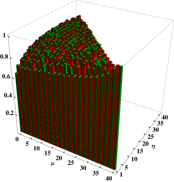
Fig. 2 shows entanglement measure of all excited states of the system with . It is observed that the excited states are all well entangled with measure in the case. The entanglement measure for both the two eigenstates in the -th band and the single eigenstate in the -th band reaches to the maximum value, i.e. for and , respectively, and the excited states in other bands with are also well entangled with . Moreover, the entanglement measure of the band-head states gradually increases with the increasing of its excitation energy or from to in the case. Additionally, except the last two bands with or , the entanglement measure of the excited states in other bands varies almost randomly with the value for as shown in Fig. 2. Therefore, the eigenstates of the 2A2S system are always well entangled.
IV SUMMARY
In this work, a systematic procedure for calculating exact solution of the 2A2S Hamiltonian is presented by using the Bethe ansatz method. It is shown that the 2A2S Hamiltonian can be expressed in terms of the generators of two copies of SU(1,1) algebra after the Jordan-Schwinger boson realization of the two related SU(2) algebras. Thus, eigenstates of the 2A2S Hamiltonian can be expressed as SU(1,1) type Bethe ansatz states, by which eigen-energies and the corresponding eigenstates are derived. To avoid solving a set of non-linear Bethe ansatz equations involved, the related extended Heine-Stieltjes polynomials are constructed, whose zeros are just components of a root of the Bethe ansatz equations. Symmetry properties of excited levels of the 2A2S system and those of zeros of the related extended Heine-Stieltjes polynomials are also discussed. As an example, the two equal spin case is analysed in detail. It is shown that the dimensional energy matrix in the uncoupled two-spin basis, where is the quantum number of the two spins, can be decomposed into dimensional bi-diagonal sub-matrices for with two-fold degeneracy for , which clearly demonstrates the advantages of the Bethe ansatz method over the direct diagonalization in the original uncoupled two-spin basis. Furthermore, in the two equal spin case, it is shown that the levels in each band labelled by are symmetric with respect to the zero energy plane perpendicular to the level diagram and that the excited states are always well entangled.
In comparison to the direct diagonalization of the 2A2S Hamiltonian in the uncoupled two-spin basis with , the size of the energy matrix increases with quadratically, while the size of the energy sub-matrices constructed by the Bethe ansatz method shown in this paper increases with linearly, which makes the diagonalization more efficient and doable for large spin cases. For example, when the two spins are large with , the diagonalization of the bidiagonal matrices with in size can be carried out on a current day computer, while the direct diagonalization of the energy matrix in the original two-spin basis with in size becomes a formidable task. Therefore, the results shown in this paper should be useful for large spin cases in Bose-Einstein condensates bec .
Further analysis of the model using the Bethe ansatz solution, such as computing the overlaps of the eigenstates with the two-spin squeezed state as suggested in 2222 and other physical quantities of the system, especially in the thermodynamic limit by using a similar procedure in cr , is beyond the scope of this paper and will be part of our future work to be presented elsewhere.
Acknowledgements.
This work was supported by National Natural Science Foundation of China (Grants No. 11675071 and No. 11775177), Australian Research Council Discovery Project DP190101529, U. S. National Science Foundation (OIA-1738287 and PHY-1913728), and LSU-LNNU joint research program with modest but important collaboration-maintaining support from the Southeastern Universities Research Association.References
- (1) M. Kitagawa and M. Ueda, Phys. Rev. A 47, 5138 (1993).
- (2) D. J. Wineland, J. J. Bollinger, W. M. Itano, F. L. Moore and D. J. Heinzen, Phys. Rev. A 46, R6797 (1992).
- (3) D. J. Wineland, J. J. Bollinger, W. M. Itano and D. J. Heinzen, Phys. Rev. A 50, R67 (1994).
- (4) A. Sørensen and K. Mømer, Phys. Rev. Lett. 86, 4431 (2001).
- (5) J. Hald, J. L. Sørensen, C. Schori and E. S. Polzik, Phys. Rev. Lett. 83, 1319 (1999).
- (6) I. D. Leroux, M. H. Schleier-Smith and V. Vuletć, Phys. Rev. Lett. 104, 073602 (2010).
- (7) C. D. Hamley, C. S. Gerving, T. M. Hoang, E. M. Bookjans and M. S. Chapman, Nature Phys. 8, 305 (2012).
- (8) H. Strobel, W. Muessel, D. Linnemann and T. Zibold, Science 345, 424 (2014).
- (9) V. Meyer, M. A. Rowe, D. Kielpinski, C. A. Sackett, W. M. Itano, C. Monroe and D. J. Wineland, Phys. Rev. Lett. 86, 5870 (2001).
- (10) J. Estéve, C. Gross, A. Weller, S. Giovanazzi and M. K. Oberthaler, Nature 455, 1216 (2008).
- (11) J. Appel, P. J. Windpassinger, D. Oblak, U. B. Hoff, N. Kjægaard and E. S. Polzik, PNAS 106, 10960 (2009).
- (12) M. H. Schleier-Smith, I. D. Leroux and V. Vuletć, Phys. Rev. Lett. 104, 073604 (2010).
- (13) M. O. Scully and M. S. Zubairy, Quantum Optics (Cambridge University, Cambridge, 1999).
- (14) M. Nielsen and I. Chuang, Quantum Computation and Quantum Information, 10th ed. (Cambridge University Press, New York, 2011).
- (15) J. Kitzinger, M. Chaudhary, M. Kondappan, V. Ivannikov, and T. Byrnes, Phys. Rev. Res. 2, 033504 (2020).
- (16) F. Pan, Y.-Z. Zhang, and J. P. Draayer, Ann. Phys. (N. Y.) 376, 182 (2017).
- (17) F. Pan, Y.-Z. Zhang, and J. P. Draayer, J. Stat. Mech., 023104 (2017).
- (18) P. Ribeiro, J. Vidal and R. Mosseri, Phys. Rev. Lett. 99, 050402 (2007).
- (19) P. Ribeiro, J. Vidal and R. Mosseri, Phys. Rev. E 78, 021106 (2008).
- (20) H. Bethe, Z. Phys. 71, 205 (1931).
- (21) M. Gaudin, J. Phys. (Paris) 37, 1087 (1976).
- (22) R. W. Richardson, Phys. Lett. 3, 277 (1963); J. Math. Phys. 6, 1034 (1965).
- (23) R. W. Richardson and N. Sherman, Nucl. Phys. 52, 221 (1964).
- (24) F. Pan and J. P. Draayer, Phys. Lett. B 451, 1 (1999).
- (25) H. Morita, H. Ohnishi, J. da Providêcia and S. Nishiyama, Nucl. Phys. B 737, 337 (2006).
- (26) Y.-H. Lee, W.-L. Yang and Y.-Z. Zhang, J. Phys. A 43, 185204 (2010).
- (27) Y.-H Lee, J. Links and Y.-Z. Zhang, Nonlinearity 24, 1975 (2011).
- (28) F. Pan, S. Yuan, Y. He, Y. Zhang, S. Yang, J. P. Draayer, Nucl. Phys. A 984, 68 (2019).
- (29) F. Pan, D. Li, S. Cui, Y. Zhang, Z. Feng, and J. P. Draayer, J. Stat. Mech., 043102 (2020).
- (30) F. Pan, L. Bao, L. Zhai, X. Cui and J. P. Draayer, J. Phys. A 44, 395305 (2011).
- (31) X. Guan, K. D. Launey, M. Xie, L. Bao, F. Pan and J. P. Draayer, Phys. Rev. C 86, 024313 (2012).
- (32) F. Pan, B. Li, Y.-Z. Zhang and J. P. Draayer, Phys. Rev. C 88, 034305 (2013).
- (33) L. Pezzé, A. Smerzi, M. K. Oberthaler, R. Schmied, and P. Treutlein, Rev. Mod. Phys. 90, 035005 (2018).
- (34) N. Kitanine, K. K. Kozlowski, J. M. Maillet, N. A. Slavnov and V. Terras, J. Stat. Mech., P04003 (2009).