Exact Hopfion Vortices in a 3D Heisenberg Ferromagnet

Introduction. Three dimensional (3D) topological solitons are of great current interest. They have recently been observed in magnetic [1], ferrroelectric [2], liquid crystal [3, 4], and other materials as well as in photonics [5], and studied in Bose-Einstein condensates [6, 7]. As is well known, solitons [8]–[11] are spatially localized, particle-like excitations that arise as solutions of nonlinear partial differential equations satisfied by the field configurations of the physical system concerned. A soliton can be non-topological or topological. Unlike the former, the latter is endowed with a nontrivial integer topological invariant, also called its topological charge. This topological property of the entity along with its energetic stability, is expected to become useful in communication technology, since these particle-like nonlinear topological excitations can serve as information carriers [5].

Various types of Heisenberg exchange models for interacting spins describing a number of magnetic materials are storehouses of solitons [12]. In the static case of the classical continuum version, a normalized spin configuration at any point $\mathbf{r}$ in physical space is described by a unit vector field $\mathbf{S}(\mathbf{r})$. Clearly, the tip of such a spin vector lies on a $2$-sphere $S^{2}$, irrespective of the spatial dimension in which it exists. In 2D, the topological solitons are the well known magnetic skyrmions. These are classified by an integer topological invariant (Pontryagin charge) $Q=(1/4\pi)\iint\mathbf{S}\cdot(\partial_{x}\mathbf{S}\times\partial_{y}\mathbf{S})\,dx\,dy$, called the winding number [8], characterizing the second homotopy group $\pi_{2}(S^{2})=Z$. First studied in 1975 by Belavin and Polyakov [13] in the context of 2D isotropic ferromagnets, they have been investigated theoretically in other magnetic models by several authors. They have also been observed experimentally in many types of 2D magnetic materials [14]. The possible role of magnetic skyrmions as bits to store information in future computer technology has been suggested [14].

In 3D, such solitons are classified by a topological invariant called the Hopf invariant $H$ (or Hopf charge), which is given by the Whitehead integral expression [15] [see Eq. (10) below]. Here $H$ can also be interpreted as the linking number of the two closed space curves in 3D physical space that are the preimages of any two distinct points on the target space $S^{2}$. Magnetic materials provide an ideal platform to create and study such topological solitons experimentally [1]. Their investigation as possible static solitons in 3D Heisenberg models is therefore of current interest. They arise as solutions of the variational equations minimizing the energy, the latter generically being nonlinear partial differential equations that are difficult to solve analytically. Hence existing theoretical work on topological solitons typically uses numerical methods as well as simulations [16]–[22]. These studies have undoubtedly yielded useful insights regarding 3D spin textures as well as the knots and links associated with them.

In the case of most micromagnetic models such as [21], the use of numerical techniques is unavoidable. On the other hand, it is instructive to identify a physically realizable magnetic model in 3D in which both the exact soliton solution as well as its corresponding Hopf invariant can be calculated analytically. Analytical methods play a crucial role in clarifying the basic physical and topological characteristics of solitons. Recently, topological solitons have been created and observed experimentally in a multilayer magnetic system [1]. A solvable model can also suggest the fabrication of appropriate magnetic materials and initiate more experiments to study the various topological aspects of these nonlinear excitations. The present work is motivated by these considerations.

Our main results are as follows: We find exact static soliton solutions for the unit spin configurations $\mathbf{S}(\mathbf{r})$ of a 3D, inhomogeneous, anisotropic Heisenberg ferromagnet. Each soliton is labeled by two integers $n$ and $m$. It is a modified skyrmion in the $z=0$ plane with winding number $n$, which twists out of the plane to become a 3D soliton. Here $m$ arises from the periodic boundary condition imposed in the $z$-direction. Using the Whitehead formula [15], we calculate its Hopf charge analytically to obtain an integer $H=nm$. It represents a hopfion vortex. ($H<0$ corresponds to a hopfion antivortex.) Using the exact solution, we plot the preimages of a few distinct points on a specific latitude of the target space $S^{2}$, and show that they are closed space curves that lie on a corresponding $2$-torus. [$\mathbf{S}(\mathbf{r})$ points in a fixed direction on a preimage curve.] These curves are either unknots or nontrivial knots, depending on $n$ and $m$. Any two of them link $nm$ times, yielding the geometric interpretation of $H$ as a linking number. Thus, this hopfion vortex is associated with a twisted, knotted, linked structure. The preimages of the points on any latitude of $S^{2}$ densely fill the surface of an associated torus. We then calculate the exact energy $E$ of the magnetic hopfion vortex. We further find that $E\geqslant cH^{1/2}$ where $c$ is a material dependent constant, showing that the topological lower bound on $E$ has a sublinear dependence on the Hopf charge. Using Derrick’s scaling analysis [23, 24], we show that the presence of the spatial inhomogeneity in the anisotropic interaction, which in turn introduces a characteristic length scale in the model, leads to the stability of the hopfion vortex.

Exact solitons for a 3D Heisenberg model. We consider the continuum version of a magnetic system described by a classical anisotropic ($XXZ$), inhomogeneous Heisenberg ferromagnet, with energy $E$ given by

$$E=(J/a)\,\iiint\big{\{}(\partial_{x}\mathbf{S})^{2}+(\partial_{y}\mathbf{S})^{2}+\widetilde{J}_{3}(\rho)(\partial_{z}\mathbf{S})^{2}\big{\}}\,dx\,dy\,dz.$$

(1)

Here $J$ is the nearest-neighbor exchange interaction in the $x$ and $y$ directions, $\widetilde{J}_{3}(\rho)=J_{3}(\rho)/J$ is the dimensionless, inhomogeneous anisotropic interaction in the $z$-direction, with $\rho=\sqrt{x^{2}+y^{2}}$, and $a$ is the lattice constant.

In what follows, we will show that an inhomogeneous anisotropy of the form $\widetilde{J}_{3}(\rho)=K_{3}\,l^{2}/\rho^{2}$ in Eq. (1) leads to exact solutions for the spin textures $\mathbf{S}(\mathbf{r})$. Here, $K_{3}$ is the strength of the anisotropy and $l$ is the length scale characterizing the inhomogeneity. In addition, this functional form also ensures the stability of the exact spin textures obtained, as will be explained in detail later.

The unit vector $\mathbf{S}$ is given in spherical polar coordinates by

$$\mathbf{S}=(\sin\Theta\,\cos\Phi,\,\sin\Theta\,\sin\Phi,\,\cos\Theta).$$

(2)

Substituting this in Eq. (1) and transforming to cylindrical coordinates $(\rho,\phi,z)$ in physical space, we get

	$\displaystyle E$	$\displaystyle=$	$\displaystyle(J/a)\iiint\!\Big{\{}\big{[}(\partial_{\rho}\Theta)^{2}+\rho^{-2}(\partial_{\phi}\Theta)^{2}\big{]}$		(3)
		$\displaystyle+$	$\displaystyle\sin^{2}\Theta\big{[}(\partial_{\rho}\Phi)^{2}+\rho^{-2}(\partial_{\phi}\Phi)^{2}\big{]}$
		$\displaystyle+$	$\displaystyle\widetilde{J}_{3}(\rho)\big{[}(\partial_{z}\Theta)^{2}+\sin^{2}\Theta\,(\partial_{z}\Phi)^{2}\big{]}\Big{\}}\rho~{}d\rho\,d\phi\,dz.$

We consider solutions of the form $\Theta=\Theta(\rho),\,\Phi=\alpha_{0}\phi+\beta_{0}z+\Phi_{0}$, where the constants $\alpha_{0}$ and $\beta_{0}$ are to be determined by the boundary conditions on $\Phi$. Equation (3) then reduces to

	$\displaystyle E$	$\displaystyle=$	$\displaystyle(J/a)\,\iiint\big{\{}\rho\,(\partial_{\rho}\Theta)^{2}$		(4)
		$\displaystyle+$	$\displaystyle\alpha_{0}^{2}\,\rho^{-1}\,\sin^{2}\Theta+\widetilde{J}_{3}(\rho)\,\beta_{0}^{2}\,\rho\,\sin^{2}\Theta\big{\}}d\rho\,d\phi\,dz\,.$

Setting $\widetilde{J}_{3}(\rho)=K_{3}\,l^{2}/\rho^{2}$ [mentioned below Eq. (1)], we find the Euler-Lagrange equation for the energy functional in Eq. (4). Then, changing variables to $\widetilde{\rho}=\ln\,(\rho/\rho_{0})$ [25] (where $\rho_{0}$ is a constant) in this equation, we obtain

$$\partial^{2}\Theta/\partial\widetilde{\rho}^{2}=\tfrac{1}{2}\left(\alpha_{0}^{2}+K_{3}\,l^{2}\,\beta_{0}^{2}\right)\sin 2\Theta\,.$$

(5)

Imposing the periodic boundary conditions $\Phi(\phi+2\pi)=\Phi(\phi)$ and $\Phi(z+L)=\Phi(z)$, we find $\alpha_{0}=n,\,\,\beta_{0}=2\pi m/L$ where $m$ and $n$ are integers. Here $L$ is a constant representing the thickness of the given 3D magnetic system. Equation (5) then yields, for the function $\widetilde{\Theta}=2\Theta$,

$\displaystyle\partial^{2}\widetilde{\Theta}/\partial\tilde{\rho}^{2}=\mu^{2}\sin\widetilde{\Theta}$

(6)

with the solution $\widetilde{\Theta}(\widetilde{\rho})=4\tan^{-1}\left(e^{\mu\widetilde{\rho}}\right)$, where

$$\mu=\pm\big{(}n^{2}+4K_{3}\pi^{2}m^{2}l^{2}/L^{2}\big{)}^{1/2}.$$

(7)

In terms of the original variables, the solution for $\Theta$ reads

$$\Theta(\rho)=2\tan^{-1}[({\rho}/\rho_{0})^{\mu}].$$

(8)

Using the above solution in Eq. (2), we arrive at the following exact static solution for the spin configuration in 3D analytically.

	$\displaystyle\mathbf{S}(\rho,\phi,z)$	$\displaystyle=$	$\displaystyle\Bigg{(}\frac{2(\rho/\rho_{0})^{\mu}}{1+(\rho/\rho_{0})^{2\mu}}\cos\,\Phi(\phi,z),$		(9)
			$\displaystyle\frac{2(\rho/\rho_{0})^{\mu}}{1+(\rho/\rho_{0})^{2\mu}}\sin\,\Phi(\phi,z),\frac{1-(\rho/\rho_{0})^{2\mu}}{1+(\rho/\rho_{0})^{2\mu}}\Bigg{)},~{}~{}$

where $\Phi(\phi,z)=n\phi+2\pi mz/L+\Phi_{0}$, with $\Phi_{0}=\Phi(0,0)$.

Clearly, the possible spin configurations $\mathbf{S}(\rho,\phi,z)$ given in Eq. (9) are labeled by two integers $n$ and $m$. It is important to note that in the solution (9), $\mu$ is defined in Eq. (7), where $K_{3},l$ and $L$ are material parameters of our model.

If $\mu<0$, then as $\rho\rightarrow 0$, we find $\Theta(\rho)\rightarrow\pi$ and $\mathbf{S}\rightarrow(0,0,-1)$; while as $\rho\rightarrow\infty$, we have $\Theta(\rho)\rightarrow 0$ and hence $\mathbf{S}\rightarrow(0,0,1)$. When $\rho=\rho_{0}$, $\Theta=\pi/2$. In the plane $z=0$, the solution becomes a modified skyrmion (resp., antiskyrmion) for $n>0$ (resp., $n<0$). (The modification arises essentially from the presence of the anisotropy $K_{3}$ with its inhomogeneity characterized by the length scale $l$, in the exponent $\mu$.) Its winding number (topological charge) $Q$ can be computed, to obtain $-n$ and $+n$, respectively [26]. An inspection of Eq. (9) shows that this skyrmion twists out into the $z$ direction in a periodic fashion $m$ times. Thus it is a 3D soliton describing a twisted skyrmion string. Such a solution has been found numerically in the context of other magnetic models [27, 19].

The occurrence of $\mu$ as the exponent of $(\rho/\rho_{0})$ in the soliton solution (9) is of significance. For a fixed $L$, the form and geometry of the topological solution we have obtained depend on the physical parameters $K_{3}$ and $l$ that appear in $\mu$, representing respectively the effects of anisotropy and inhomogeneity in the interacting system of spins. The presence of $\mu$ enables us to control the rate of change of $\Theta(\rho)$ with $\rho$ in the soliton solution, by tuning these material parameters. This in turn should be helpful in designing experiments to create and observe the twisted 3D soliton. Usually, in a given experiment it is convenient to keep $K_{3}$ and $L$ fixed, and examine the 3D spin textures for various length scales $l$ of the inhomogeneity. Indeed, one way to change $l$ systematically is to vary the (functionally graded) doping profile in the $(x,y)$ plane appropriately, in experiments.

For completeness, we point out that if $\mu>0$ in Eq. (9), the spin configuration for $z=0$ corresponds to $\mathbf{S}\rightarrow(0,0,1)$ as $\rho\rightarrow 0$, while $\mathbf{S}\rightarrow(0,0,-1)$ as $\rho\rightarrow\infty$. Some authors [14] use this alternative boundary condition to define a skyrmion. All the results in the foregoing discussion hold good for both conventions.

Calculation of the Hopf invariant $H$. As mentioned in the Introduction, $H$ can be calculated from the Whitehead formula [15, 28]

$$H=-(1/8\pi^{2})\iiint(\mathbf{A}\cdot\mathbf{B})\,dx\,dy\,dz,$$

(10)

where the Cartesian components of the emergent magnetic field [1] are given by $B_{x}=-\mathbf{S}\cdot(\partial_{y}\mathbf{S}\times\partial_{z}\mathbf{S})$ and cyclic permutations for $B_{y}$ and $B_{z}$, and $\mathbf{A}$ is the corresponding vector potential. It is easily verified that $\nabla.\mathbf{B}=0$. Using the solution (9) and expressing the Cartesian components of $\mathbf{B}$ in cylindrical polar coordinates in physical space, we get

	$\displaystyle B_{x}=\beta_{0}(\partial_{\rho}\cos\Theta)\sin\phi\,,~{}~{}B_{y}=-\beta_{0}(\partial_{\rho}\cos\Theta)\cos\phi\,,$
	$\displaystyle B_{z}=(\alpha_{0}/\rho)\partial_{\rho}\cos\Theta.$		(11)

Solving $\nabla\times\mathbf{A}=\mathbf{B}$ for the Cartesian components of $\mathbf{A}$ using the appropriate boundary conditions on $\Theta(\rho)$ [as described below Eq. (9)], a lengthy but straightforward calculation yields

	$\displaystyle A_{x}=-(\alpha_{0}/\rho)(\cos\,\Theta\pm 1)\sin\,\phi,\,$
	$\displaystyle A_{y}=(\alpha_{0}/\rho)(\cos\,\Theta\pm 1)\cos\,\phi,\,~{}~{}A_{z}=\beta_{0}\cos\,\Theta.$		(12)

The $\pm$ signs correspond to $\mu>0$ and $\mu<0$, respectively. Substituting Eq. (11) and Eq. (12) in Eq. (10), the Hopf invariant of the 3D soliton can be written in the form

$$H=\mp\frac{\alpha_{0}\beta_{0}}{8\pi^{2}}\int_{0}^{L}\!dz\int_{0}^{2\pi}\!d\phi\!\int_{0}^{\pi}\sin\,\Theta\,d\Theta.$$

(13)

Since $\alpha_{0}=n$ and $\beta_{0}=2\pi m/L$, we obtain

$$H=nm,$$

(14)

keeping in mind that $n$ can be a positive or negative integer. Interestingly, this integer $H$ emerges as a product of two integers in our spin system. Note that both $m$ and $n$ have to be nonzero integers for the Hopf charge $H$ to be nonzero.

Usually, a 3D topological soliton is called a hopfion if it satisfies uniform boundary conditions [e.g., ${\bf S}({\bf r}\rightarrow\infty)$ =$(0,0,1)$], so that the 3D physical space can be compactified to $S^{3}$. It represents a map $\mathbf{S}:S^{3}\rightarrow S^{2}$. Its Hopf invariant is an integer characterizing the third homotopy group $\pi_{3}(S^{2})$. On the other hand, our soliton solution Eq. (9) described by a twisted skyrmion string is obtained using the homogeneous boundary condition for $\mathbf{S}$ in each $z={\rm constant}$ plane, together with the periodicity in the $z$-direction. This represents a map $\mathbf{S}:S^{2}\times T^{1}\rightarrow S^{2}$ [29]. Due to this difference, our twisted skyrmion string given in Eq. (9) is called a hopfion vortex rather than a hopfion. As seen from Eq. (14), its integer Hopf invariant is obtained as the product of the winding number $n$ of the skyrmion in the $xy$ plane, and the integer $m$ giving the number of times it winds around the $z$-axis till it reaches the boundary at $z=L$. These integers encode, respectively, the topology of the $S^{2}$ and $T^{1}$ parts of the manifold $S^{2}\times T^{1}$. Since $H$ in Eq. (14) can have either sign, the system supports both hopfion vortices and hopfion antivortices.

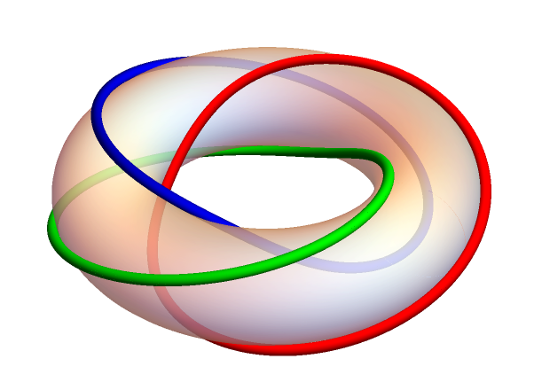
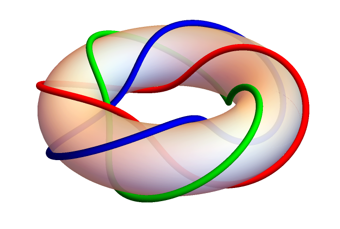
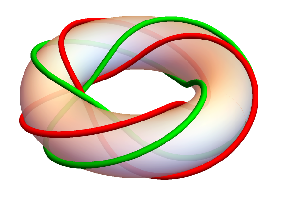
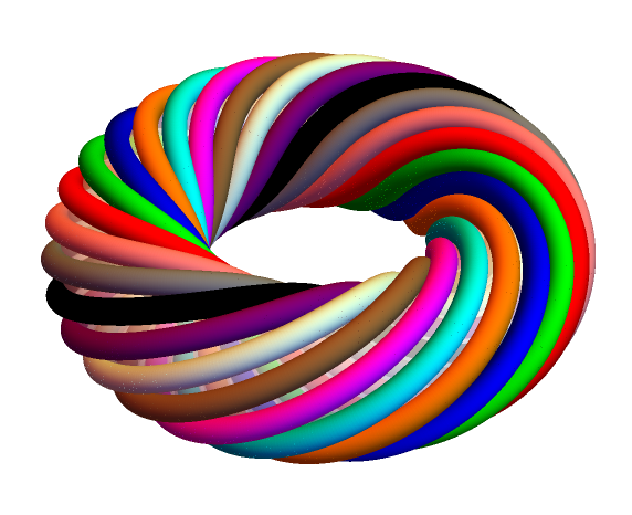
Knotted structure of the hopfion vortex and Hopf invariant as a linking number. Next, we use Mathematica to find the preimage of any specific point on $S^{2}$, i.e., the points in 3D space corresponding to a specific value $(\Theta,\Phi)$ of $\mathbf{S}(\mathbf{r})$ of the hopfion vortex solution (9). We have plotted the three preimage curves corresponding to $\Theta=\pi/2$ and $\Phi=0,\pi/3$ and $2\pi/3$, for the cases (i) $n=1,m=1$ [Fig. 1(a)], (ii) $n=1,m=2$ [Fig. 1(b)], and (iii) $n=2,m=3$ [Fig, 1(c)]. As these illustrative examples show, each of the preimages is a closed space curve which is, in cases (i) and (ii), an unknot, topologically equivalent to a circle. In contrast, it is a trefoil knot (a nontrivial knot) in case (iii). Further, as can be readily seen in Fig. 1, each closed curve lies on the surface of a torus, traversing $n$ times around the poloidal direction and $m$ times around the toroidal direction. The analytical result of Eq. (14) gives $H=1,2,6$, respectively in cases (i), (ii) and (iii). Correspondingly, we see from Fig. 1 that any two closed space curves link once, twice and six times, respectively, in these three cases. This corroborates geometrically that the Hopf invariant $H$ is precisely just the linking number of the preimages of two distinct points on $S^{2}$. For a given value of $\Theta$, the preimages of the points $\Phi\in[0,2\pi)$ densely fill the corresponding torus (Fig. 2). As is well known [30], a torus knot is an unknot if and only if either $n$ or $m$ is $\pm 1$, and a nontrivial knot if $m$ and $n$ are coprime. Our plots illustrate the knotted and linked structure of the hopfion vortex.

Exact energy of the hopfion vortex and its topological lower bound. Setting $\widetilde{J}_{3}=K_{3}l^{2}/\rho^{2}$ in Eq. (4), using the definition of $\mu$ from Eq. (7) and putting in the appropriate limits of integration, the energy of the hopfion vortex is given by

$$E=(J/a)\int_{0}^{L}\!dz\int_{0}^{2\pi}\!d\phi\int_{0}^{\infty}\!\big{\{}\rho(\partial_{\rho}\Theta)^{2}+\mu^{2}\rho^{-1}\sin^{2}\Theta\big{\}}\,d\rho\,.$$

(15)

Using Eq. (8) for $\Theta(\rho)$, a short calculation yields

$$E=\frac{16\pi JL}{a}\,{\mu}^{2}\rho_{0}^{2\mu}\,\int_{0}^{\infty}\,\frac{\rho^{(2\mu-1)}}{[\rho_{0}^{2\mu}+\rho^{2\mu}]^{2}}\,d\rho=(8\pi JL/a)\,|\mu|.$$

(16)

Substituting for $\mu$ from Eq. (7), the energy of the hopfion vortex is given by the exact expression

$$E(n,m)=(8\pi JL/a)\big{(}n^{2}+4\pi^{2}K_{3}l^{2}m^{2}/L^{2}\big{)}^{1/2}.$$

(17)

Since $E(n,m)=E(-n,m)$, hopfion vortex and hopfion antivortex have the same energy.

We write Eq. (17) as

$$E(n,m)=(8\pi JL/a)\big{(}n^{2}+\beta^{2}\,m^{2}\big{)}^{1/2},$$

(18)

where we have defined

$$\beta=2\pi\sqrt{K_{3}}(l/L).$$

(19)

Substituting the inequality $\big{(}n^{2}+\beta^{2}m^{2}\big{)}\geqslant 2\beta mn$ in Eq. (18), and using $mn=H$, we get

$$E(n,m)\geqslant c\sqrt{H},$$

(20)

where $c=2^{4}\pi^{3/2}K_{3}^{1/4}J\sqrt{lL}/a$. Thus, the lower bound of the energy of the hopfion vortex has a sublinear dependence on its topological charge $H$. This is in contrast to the well known lower energy bound for the skyrmion (a 2D topological soliton) which is linear in the Pontryagin charge $Q$. Such a sublinear behavior is usually attributed [31] to the knotted and linked preimages, which is the source of the charge $H$ of a 3D topological soliton [32].

Stability. Before investigating the stability of our 3D hopfion vortex solution given in Eq. (9), we first carry out the general Hobart-Derrick scaling analysis [23, 24] for the energy expression $E$ given in Eq. (1), after substituting the inhomogeneous anisotropy $\widetilde{J}_{3}(\rho)=K_{3}l^{2}/\rho^{2}$ in it [33].

It is convenient to write the first two terms of the energy [Eq. (1)] as

$$(J/a)\,\iiint[(\partial_{x}\mathbf{S})^{2}+(\partial_{y}\mathbf{S})^{2}]dx\,dy\,dz=A_{0},$$

(21)

and its last term as

$$(J/a)\,\iiint[K_{3}\,l^{2}/(x^{2}+y^{2})]\,(\partial_{z}\mathbf{S})^{2}\,dx\,dy\,dz=B_{0},$$

(22)

where we have used $\rho^{2}=(x^{2}+y^{2})$. Derrick’s scaling analysis [24] involves letting $(x,y,z)$ to $(\lambda\,x,\lambda\,y,\lambda\,z)$ in the energy expression of Eq. (1), $\lambda$ being the scale factor. This yields

$$E(\lambda)=\lambda\,A_{0}\,+\,(1/\lambda)\,B_{0}\,.$$

(23)

To analyze the extrema of $E(\lambda)$, we set $dE/d\lambda=A_{0}-(1/\lambda^{2})\,B_{0}\,=\,0$. This can have a positive solution $\lambda_{1}=+\sqrt{(B_{0}/A_{0})}$, where $A_{0}$ and $B_{0}$ are integrals defined in Eqs. (21) and (22) above. Note that $A_{0}$ is always positive and $B_{0}$ is positive for $K_{3}>0$, as considered in our model. Also note that $B_{0}$ has a multiplicative factor that depends on $l^{2}$. It can be easily verified that $d^{2}E/d\lambda^{2}=[2/(\lambda_{1})^{3}]B_{0}$ is positive for any finite value of $l$, showing that $E(\lambda)$ has a minimum at $\lambda_{1}$. This implies that there is generic stability in this inhomogeneous anisotropic system.

Next, we demonstrate the stability of the specific case of our hopfion vortex solutions for ${\bf S}$ given in Eq. (9), by computing the corresponding integrals $A_{0}$ and $B_{0}$ for these solutions explicitly. Our detailed (and somewhat lengthy) calculations yield

$$\lambda_{1}=\sqrt{B_{0}/A_{0}}=\beta m/\sqrt{[2n^{2}+\beta^{2}m^{2}]},$$

(24)

where $\beta$ is given in Eq. (19). It is readily seen that in experiments with a fixed $K_{3}$ and $L$, for a suitable choice of $l$, $\beta$ is finite and fixed. Hence from Eq. (24), the scale $\lambda_{1}$ is seen to be finite for all nonzero integers $m$ and $n$. This shows that the hopfion vortex solutions supported by the inhomogeneous anisotropic ferromagnet will not shrink or flatten out, establishing their stability.

Note that the presence of the characteristic length $l$ of the inhomogeneity in the anisotropic term plays an important role in the stability of 3D spin textures. This is reminiscent of several 2D models of spin systems where the introduction of a characteristic length in the system via diverse physical mechanisms [25, 34] typically leads to the stabilization of 2D spin textures.

We parenthetically remark that a homogeneous anisotropy corresponds to setting $\widetilde{J}_{3}(\rho)=(J_{3}/J)$ in the second term in the energy [Eq. (1)]. It is easily verified that Derrick’s scaling analysis in this case will lead to $E(\lambda)=\lambda(\,A_{0}\,+\,B_{0}\,)$ [instead of Eq. (23)], showing that there is no minimum value for $E$ for any $\lambda$. This confirms the well known result that the solutions of a homogeneous anisotropic Heisenberg ferromagnet are generically unstable.

We also mention that our scaling analysis given above, which proves the stability of solitons in a 3D magnet in the presence of an inhomogeneous anisotropy, is similar to the analysis usually given [35] for proving the stability of skyrmions in an anisotropic 2D magnet in the presence of a Dzyaloshinskii-Moriya interaction term. It has been shown in the case of 3D chiral ferromagnets [20] and chiral ferromagnetic fluids [36] that the presence of the Dzyaloshinskii-Moriya [37] interaction term of the form $D\,\mathbf{S}\cdot(\nabla\times\mathbf{S})$ in the energy plays an important role in stabilizing the soliton. Turning to nonchiral (inversion symmetric) 3D ferromagnets, it is reasonable to expect that continuum Heisenberg models with competing energy terms could lead to stable solitons. However, identifying appropriate terms which would yield a stable 3D soliton solution which also has an integer Hopf invariant (as we have, in our model) is far from obvious.

Discussion. The main results obtained in this paper have already been summarized in the Introduction. Our results are novel and we believe they open up new avenues of investigation, e.g. hopfion vortex lattice solutions of the model, study of the effects of an applied magnetic field, topological transitions in spin textures, Berry phase phenomena and the dynamics of hopfion vortices.

The introduction of an inhomogeneity in the exchange interaction in a Heisenberg model was motivated in part by an earlier work [38] on the dynamics of the continuum model of an isotropic Heisenberg chain with an inhomogeneous exchange interaction, which supports stable 1D solitons for certain specific inhomogeneities. Since then, various aspects of inhomogeneous magnetic systems have been studied by several other authors [39].

We remark in passing that the results we have presented for the continuum Heisenberg model should be applicable in fields other than magnetism, where the corresponding energy density involves inhomogeneous, anisotropic generalizations of $|\nabla\mathbf{n}|^{2}$, where $\mathbf{n}$ is a unit vector field. The energy density of the nonlinear sigma model [8], the splay term in the free energy of liquid crystals [4], the curvature term in the elastic rod energy [40], etc. are some examples.

Theoretical and experimental studies of topological solitons in 3D Heisenberg models have started to gain momentum in recent years. There is a recent numerical study [27] on twisted skyrmions which become hopfion vortices for appropriate boundary conditions. Hopfions have been identified in chiral ferromagnetic fluids [36] and observed [1] in magnetic multilayer systems. Based on their nanometer to micrometer sizes in various magnetic materials as well as their topological and energy-based stability, the possible application of topological solitons in future computer technology has been recognized. They can be used to store bits of information, where a bit corresponds to the presence or absence of a topological soliton. Certain dynamical advantages of 3D localized entities over skyrmions as information carriers have also been pointed out [22, 5]. Thus, one could envisage such distinct applications as hopfionics akin to the field of skyrmionics [14].

We conclude by pointing out that our magnetic model is not just an exactly solvable theoretical model that reveals all the topological aspects of the 3D topological solitons obtained by us succinctly, but is also useful in designing novel experiments to observe them. Specifically, we note that the $J_{3}$ term in the energy Eq. (1) has the same effect as a perpendicular magnetic anisotropy (PMA) term $KS_{z}^{2}$ used in experiments. Topological solitons have been studied in Ir/Co/Pt nano-disc multilayered systems, with the PMA term $K$ varying spatially over each layer, with a linear dependence [1]. Our results suggest that layers with a circularly symmetric inverse square dependence $1/\rho^{2}$ of the inhomogeneity in the anisotropy $\widetilde{J}_{3}$ will lead to stable hopfion vortices with a range of $H$ values. Some suggestions with regard to fabricating inhomogeneous magnetic materials have been made in [38].

Finally, we note that the inverse square interaction of our model that has led to exact solvability is reminiscent of a similar interaction between particles in the well known Calogero-Moser model which is known to be completely integrable, with connections to diverse fields [41]. Hence our work has potential ramifications for other physical systems as well.

We hope that our results will motivate the fabrication of inhomogeneous, anisotropic 3D magnetic materials that are described by our model, so that the exact hopfion vortex solutions predicted by it can be created in the laboratory and their possible applications in nanotechnology investigated.

References

- [1] N. Kent et al., Nature Commun. 12, 1562 (2021).
- [2] I. Luk’yanchuk, Y. Tikhonov, A. Razumnava, and V. M. Vinokur, Nature Commun. 11, 2433 (2020).
- [3] P. J. Ackerman and I. I. Smalyukh, Nature Commun. 12, 1562 (2021).
- [4] P. J. Ackerman and I. I. Smalyukh, Phys. Rev. X 7, 011006 (2017).
- [5] Y. Shen, B. Yu, H. Wu, C. Li, Z. Zhu, and A. V. Zayats, Adv. Photonics 5, 015001 (2023).
- [6] Y. M. Bidasyuk et al., Phys. Rev. A 92, 053603 (2015).
- [7] S. Zou et al., Phys. Fluids 33, 027105 (2021).
- [8] R. Rajaraman, Solitons and Instantons (North-Holland, Amsterdam, 1982).
- [9] N. Manton and P. Sutcliffe, Topological Solitons (Camb. Univ. Press, Cambridge, 2004), and references therein.
- [10] T. Dauxois and M. Peyard, Physics of Solitons (Camb. Univ. Press, Cambridge, 2006).
- [11] Y. M. Shnir, Topological and Nontopological Solitons in Scalar Field Theories (Camb. Univ. Press, Cambridge, 2018).
- [12] A. M. Kosevich, B. A. Ivanov, and A. S. Kovalev, Phys. Rep. 194, 117 (1990).
- [13] A. A. Belavin and A. M. Polyakov, JETP Lett. 22, 245 (1975).
- [14] For reviews of magnetic skyrmions see, e.g., N. Nagaosa and Y. Tokura, Nat. Nanotechnol. 8, 899 (2013); A. Fert, N. Reyren, and V. Cros, Nat. Rev. Mater. 2, 17031 (2017); B. Göbel, I. Mertig, and O. A. Tretiakov, Phys. Rep. 895, 1 (2021), and references therein.
- [15] J. H. C. Whitehead, Proc. Nat. Acad. Sci. (USA) 33, 117 (1947).
- [16] P. Sutcliffe, Phys. Rev. Lett. 118 247203 (2017).
- [17] P. Sutcliffe, Nat. Mater. 16, 392 (2017).
- [18] P. Sutcliffe, Rev. Math. Phys. 30, 1840017 (2018).
- [19] M. Kobayashi and M. Nitta, Phys. Lett. B 728, 314 (2014).
- [20] Y. Liu, R. K. Lake, and J. Zang, Phys. Rev. B 98, 174437 (2018).
- [21] F. N. Rybakov, N. S. Kiselev, A. B. Borisov, L. Döring, C. Melcher, and S. Blügel, APL Mater. 10, 111113 (2022); arXiv:1904.00250.
- [22] X. S. Wang, A. Quaimzadeh, and A. Brataas, Phys. Rev. Lett. 123, 147203 (2019).
- [23] R. H. Hobart, Proc. Phys. Soc. 82, 201 (1963)
- [24] G. M. Derrick, J. Math. Phys. 5, 1252 (1964).
- [25] A. Saxena and R. Dandoloff, Phys. Rev. B 66, 104414 (2002).
- [26] See, e.g., W. Koshibae and N. Nagaosa, Nat. Commun. 7, 10542 (2016).
- [27] See, e.g., T. Yokota, J. Phys. Soc. Jpn. 90, 104701 (2021).
- [28] J. Gladikowski and M. Helmund, Phys. Rev. D 56, 5194 (1997).
- [29] J. Jaykka and J. Hietarinta, Phys. Rev. D 79, 125027 (2009) and references therein.
- [30] See, e.g., C. Oberti and L. Ricca, J. Knot Theory Ramif. 25, 1650036 (2016).
- [31] R. S. Ward, J. Math. Phys. 59, 022904 (2018).
- [32] We note here that the lower bound of the energy has a sublinear behavior in the Faddeev-Skyrme model as well; however it goes as [11] in this model which supports hopfions rather than hopfion vortices.
- [33] It must be noted that Derrick’s scaling [24] is always applied to the given energy expression of the system, and that the general analysis is independent of the specific boundary conditions that may be subsequently used to obtain explicit solutions supported by it.
- [34] R. Dandoloff and A. Saxena, Recent Res. Devel. Physics 6, 429 (2005); R. Dandoloff, J. Mod. Phys. 11, 1326 (2020).
- [35] A.O. Leonov et al., New J. Phys. 18, 065003 (2016).
- [36] P. J. Ackerman and I. I. Smalyukh, Nat. Mater. 16, 426 (2017).
- [37] I. Dzyaloshinskii, J. Phys. Chem. Solids 4, 241 (1958); T. Moriya, Phys. Rev. 120, 91 (1960).
- [38] Radha Balakrishnan, J. Phys C. 15, L1305 (1982).
- [39] See, e.g., Z-H. Zhang et al. J. Phys. Soc. Jpn. 75, 104002 (2006); K. H. Han and H. J. Shin, J. Phys. A: Math. Theor. 40, 979 (2007); K. Abhinav and P. Guha, Eur. Phys. J. B 91, 52 (2018); M. Saravanan and W. B. Cardoso, Commun. Nonlinear Sci. Numer. Simulat. 69, 176 (2019); Y-J. Zhang, D. Zhao, and Z-D. Li, Commun. Theor. Phys. 73, 015105 (2021).
- [40] D. Harland, M. Speight, and P. Sutcliffe, Phys. Rev. D 83, 065008 (2011).
- [41] F. Calogero, J. Math. Phys. 12, 419 (1971) [Erratum, ibid; 3646 (1996)]; J. Moser, Advances in Math. 16, 197 (1975); See also, P. Etingof, Lectures on Calogero-Moser Systems, arXiv:math/0606233.