Ex-Ray: Distinguishing Injected Backdoor from Natural Features in Neural Networks by Examining Differential Feature Symmetry
Abstract
Backdoor attack injects malicious behavior to models such that inputs embedded with triggers are misclassified to a target label desired by the attacker. However, natural features may behave like triggers, causing misclassification once embedded. While they are inevitable, mis-recognizing them as injected triggers causes false warnings in backdoor scanning. A prominent challenge is hence to distinguish natural features and injected backdoors. We develop a novel symmetric feature differencing method that identifies a smallest set of features separating two classes. A backdoor is considered injected if the corresponding trigger consists of features different from the set of features distinguishing the victim and target classes. We evaluate the technique on thousands of models, including both clean and trojaned models, from the TrojAI rounds 2-4 competitions and a number of models on ImageNet. Existing backdoor scanning techniques may produce hundreds of false positives (i.e., clean models recognized as trojaned). Our technique removes 78-100% of the false positives (by a state-of-the-art scanner ABS) with a small increase of false negatives by 0-30%, achieving 17-41% overall accuracy improvement, and facilitates achieving top performance on the leaderboard. It also boosts performance of other scanners. It outperforms false positive removal methods using L2 distance and attribution techniques. We also demonstrate its potential in detecting a number of semantic backdoor attacks.
1 Introduction
Backdoor attack (or trojan attack) to Deep Learning (DL) models injects malicious behaviors (e.g., by data poisoning [32, 50, 46, 9] and neuron hijacking [49]) such that a compromised model behaves normally for benign inputs and misclassifies to a target label when a trigger is present in the input. Depending on the form of triggers, there are patch backdoor [32] where the trigger is a pixel space patch; watermark backdoor [49] where the trigger is a watermark spreading over an input image, filter backdoor [48] where the trigger is an Instagram filter, and reflection attack [50] that injects semantic trigger through reflection (like through a piece of reflective glass). More discussion of existing backdoor attacks can be found in a few comprehensive surveys [44, 51, 28]. Backdoors are a prominent threat to DL applications due to the low complexity of launching such attacks, the devastating consequences especially in safety/security critical applications, and the difficulty of defense due to model uninterpretability.
There are a body of existing defense techniques. Neural Cleanse (NC) [77] and Artificial Brain Stimulation (ABS) [48] make use of optimization to reverse engineer triggers and determine if a model is trojaned. Specifically for a potential target label, they use optimization to find a small input pattern, i.e., a trigger, that can cause any input to be classified as the target label when stamped. DeepInspect [17] uses GAN to reverse engineer trigger. These techniques leverage the observation that triggers are usually small in order to achieve stealthiness during attack such that a model is considered trojaned if small triggers can be found. In [38, 24], it was observed that clean and trojaned models have different behaviors under input perturbations, e.g., trojaned models being more sensitive. Such differences can be leveraged to detect backdoors. More discussion of existing defense techniques can be found in Section 5.


Although existing techniques have demonstrated effectiveness in various scenarios, an open problem is to distinguish natural and benign features that can act as backdoors, called natural backdoors in this paper, from injected backdoors. As demonstrated in [48], natural backdoors may exist in clean models. They are usually activated using strong natural features of the target label as triggers, called natural triggers in this paper. Fig. 1 presents a clean ImageNet model downloaded from [2] with a natural trigger. Figure (a) presents a clean sample of hummingbird stamped with a small 2525 natural trigger at the top-left corner; (b) shows a zoom-in view of the trigger; and (c) a sample in the target class (i.e., junco bird). Observe that the trigger demonstrates natural features of the target (e.g., eyes and beak of junco). The trigger can induce misclassification in 78% of the hummingbird samples. In other words, natural backdoors are due to natural differences between classes and hence inevitable. For instance, replacing 80% area of any clean input with a sample of class very likely causes the model to predict . The 80% replaced area can be considered a natural trigger. Natural backdoors share similar characteristics as injected backdoors, rendering the problem of distinguishing them very challenging. For instance, both NC and ABS rely on the assumption that triggers of injected backdoors are very small. However, natural triggers could be small (as shown by the above example) and injected triggers could be large. For example in semantic data poisoning [9], reflection attack [50], hidden-trigger attack [64] and composite attack [46], injected triggers can be as large as any natural object. In the round 2 of TrojAI backdoor scanning competition111TrojAI is a multi-year and multi-round backdoor scanning competition organized by IARPA [4]. In each round, a large number of models of different structures are trojaned with various kinds of triggers, and mixed with clean models. Performers are supposed to identify the trojaned models. Most aforementioned techniques are being used or have been used in the competition., many models (up to 40% of the 552 clean models) have natural backdoors that are hardly distinguishable from injected backdoors, causing a large number of false positives for performers. Examples will be discussed in Section 2.

injected_trigger


trigger_by_ABS


Distinguishing natural backdoors from injected ones is critical due to the following reasons. (1) It avoids false warnings, which may be in a large number due to the prevalence of natural triggers. For example, any models that separate the aforementioned two kinds of birds may have natural backdoors between the two classes due to their similarity. That is, stamping any hummingbird image with junco’s beak somewhere may cause the image to be classified as junco, and vice versa. However, the models and the model creators should not be blamed for these inevitable natural backdoors. A low false warning rate is very important for traditional virus scanners. We argue that DL backdoor scanners should have the same goal. (2) Being correctly informed about the presence of backdoors and their nature (natural or injected), model end users can employ proper counter measures. For example, since natural backdoors are inevitable, the users can use these models with discretion and have tolerance mechanism in place. In contrast, models with injected backdoors are just malicious and should not be used. We argue that in the future, when pre-trained models are published, some quality metrics about similarity between classes and hence natural backdoors should be released as part of the model specification to properly inform end users. (3) Since model training is very costly, users may want to fix problematic models instead of throwing them away. Correctly distinguishing injected and natural backdoors provides appropriate guidance in fixing. Note that the former denotes out-of-distribution behaviors, which can be neutralized using in-distribution examples and/or adversarial examples. In contrast, the latter may denote in-distribution ambiguity (like cats and dogs) that can hardly be removed, or dataset biases. For example, natural backdoors in between two classes that are not similar (in human eyes) denote that the dataset may have excessive presence of the corresponding natural features. The problem can be mitigated by improving datasets. As we will show in Section 4.6, injected backdoors are easier to mitigate than natural backdoors.
We develop a novel technique to distinguish natural and injected backdoors. We use the following threat model.
Threat Model. Given a set of models, including both trojaned and clean models, and a small set of clean samples for each model (covering all labels), we aim to identify the models with injected backdoor(s) that can flip samples of a particular class, called the victim class, to the target class. The threat model is more general than the typical universal attack model in the literature [77, 48, 41], in which backdoors can induce misclassification for inputs of any class. We assume the models can be trojaned via different methods such as pixel space, feature space data poisoning (e.g., using Instagram filters as in TrojAI), composite attack, reflection attack, and hidden-trigger attack. According to the definition, the solution ought to prune out natural backdoor(s).
We consider backdoors, regardless of natural or injected, denote differences between classes. Our overarching idea is hence to first derive a comprehensive set of natural feature differences between any pair of classes using the provided clean samples; then when a trigger is found between two classes (by an existing upstream scanner such as ABS), we compare if the feature differences denoted by the trigger is a subset of the differences between the two classes. If so, the trigger is natural. Specifically, let be a layer where features are well abstracted. Given samples of any class pair, say and , we aim to identify a set of neurons at such that (1) if we replace the activations of the samples at those neurons with the corresponding activations of the samples, the model will classify these samples to ; (2) if we replace the activations of the samples at the same set of neurons with the corresponding activations of the samples, the model will classify the samples to . We call the conditions the differential feature symmetry. We use optimization to identify the smallest set of neurons having the symmetry. We call it the differential features or mask in this paper. Intuitively, the features in the mask define the differences between the two classes. Assume some existing backdoor scanning technique is used to generate a set of triggers. Further assume a trigger causes all samples in to be misclassified to . We then leverage the aforementioned method to compute the mask between samples and samples, i.e., the samples stamped with . Intuitively, this mask denotes the features in the trigger. The trigger is considered natural if its mask shares substantial commonality with the mask between and .
Our contributions are summarized as follows.
-
•
We study the characteristics of natural and injected backdoors using TrojAI models and models with various semantic backdoors.
-
•
We propose a novel symmetric feature differencing technique to distinguish the two.
-
•
We implement a prototype Ex-Ray, which stands for (“Examining Differential Feature Symmetry”). It can be used as an addon to serve multiple upstream backdoor scanners.
-
•
Our experiments using ABS+Ex-Ray on TrojAI rounds 2-4 datasets222Round 1 dataset is excluded due to its simplicity. (each containing thousands of models), a few ImageNet models trojaned by data poisoning and hidden-trigger attack, and CIFAR10 models trojaned by composite attack and reflection attack, show that our method is highly effective in reducing false warnings (78-100% reduction) with the cost of a small increase in false negatives (0-30%), i.e., injected triggers are undesirably considered as natural. It can improve multiple upstream scanners’ overall accuracy including ABS (by 17-41%), NC (by 25%), and Bottom-up-Top-down backdoor scanner [1] (by 2-15%). Our method also outperforms other natural backdoor pruning methods that compare L2 distances and leverage attribution/interpretation techniques. It allows effective detection of composite attack, hidden-trigger attack, and reflection attack that are semantics oriented (i.e., triggers are not noise-like pixel patterns but rather objects and natural features).
-
•
On the TrojAI leaderboard, ABS+Ex-Ray achieves top performance in 2 out of the 4 rounds up to the submission day, including the most challenging round 4, with average cross-entropy (CE) loss around 0.32333The smaller the better. and average AUC-ROC444An accuracy metric used by TrojAI, the larger the better. around 0.90. It successfully beat all the round targets (for both the training sets and the test sets remotely evaluated by IARPA), which are a CE loss lower than 0.3465 More can be found in Section 2.
2 Motivation
In this section, we use a few cases in TrojAI round 2 to study the characteristics of natural and injected backdoors and explain the challenges in distinguishing the two. We then demonstrate our method.
According to the round 2 leader-board [4, 5], most performers cannot achieve higher than 0.80 AUC-ROC, suffering from substantial false positives. In this round, TrojAI models make use of 22 different structures such as ResNet152, Wide-ResNet101 and DenseNet201. Each model is trained to classify images of 5-25 classes. Clean inputs are created by compositing a foreground object, e.g., a synthetic traffic sign, with a random background image from the KITTI dataset [30]. An object is usually a shape with some symbol at the center. Half of the models are poisoned by stamping a polygon to foreground objects or applying an Instagram filter. Random transformations, such as shifting, titling, lighting, blurring, and weather effects, may be applied to improve diversity. Fig. 2 (a) to (c) show model #7 in round 2, with (a) presenting a victim class sample stamped with a polygon trigger in purple, (b) a target class sample, (c) the trigger generated by ABS555Our technique requires an upstream trigger generation technique, such as ABS and NC [77]. ABS [48] works by optimizing a small patch in the input space that consistently flips all the samples in the victim class to the target class. It samples internal neuron behaviors to determine the possible target labels for search space reduction. . Observe that the trigger is much smaller than the foreground objects and hence ABS can correctly determines there is a backdoor. However, there are foreground object classes similar to each other such that the features separating them could be as small as the trigger. Figures (d) and (e) show two different foreground object classes in model #123 (a clean model). Observe that both objects are blue octagons. The differences lie in the small symbols at the center of octagons. When scanning this pair of classes to determine if samples in (d) can be flipped to (e) by a trigger, ABS finds a (natural) trigger as shown in figure (f). Observe that the trigger has pixel patterns resembling the symbol at the center of (e). Both ABS and NC report model #123 as trojaned (and hence a false positive) since they cannot distinguish the natural trigger from injected ones due to their similar sizes.

Besides object classes being too similar to each other, another reason for false positives in backdoor scanning is that injected triggers could be large and complex. To detect such backdoors, optimization based techniques have to use a large size-bound in trigger reverse engineering, which unfortunately induces a lot of false positives, as large-sized natural triggers can be easily found in clean models. According to our analysis, the size of injected triggers in the 276 TrojAI round 2 models trojaned with polygon triggers ranges from 85 to 3200 pixels. Figure 3 shows the number of false positives generated by ABS when the maximum trigger (to reverse engineer) varies from 400 to 3200 pixels. Observe that the number of false positives grows substantially with the increase of trigger size. When the size is 3200, ABS may produce over 400 false positives among the 552 clean models.


In addition, there are backdoor attacks that inject triggers as large as regular objects. For example, composite attack [46] injects backdoor by mixing existing benign features from two or more classes. Fig. 4 shows a composite attack on a face recognition model trained on the Youtube Face dataset [81]. Figure (a) shows an image used in the attack, mixing two persons and having the label set to that of (b). Note that the trigger is no longer a fixed pixel pattern, but rather the co-presence of the two persons or their features. Figure (c) shows an input that triggers the backdoor. Observe that it contains the same two persons but with different looks from (a). As shown in [46], neither ABS nor NC can detect such attack, as using a large trigger setting in reverse-engineering, which is needed for this scenario, produces too many false positives.
Note that although perturbation based scanning techniques [24, 38] do not require optimization, they suffer from the same problem, as indicated by the leaderboard results. This is because if benign classes are similar to each other, their classification results are as sensitive to input perturbations as classes with backdoor, causing false positives in scanning; if triggers are large, the injected misclassification may not be so sensitive to perturbation, causing false negatives.


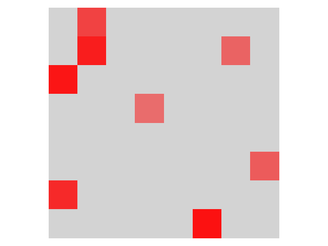
Our Method. Given a trigger generated by some upstream optimization technique that flips samples in victim class to target class , our technique decides if it is natural by checking if the trigger is composed of features that distinguish and . This is achieved by a symmetric feature differencing method. The method identifies a set of features/neurons (called mask) such that copying their values from one class to another flips the classification results. Fig. 5 (a) shows the mask in the second last convolutional layer of the TrojAI round 2 trojaned model #7 (i.e., the model in Fig. 2 (a)-(c)). It distinguishes the victim and target classes. Note that a mask is not specific to some input sample, but rather to an pair of classes. Each block in the mask denotes a feature map (or a neuron) with red meaning that the whole feature map needs to be copied (in order to flip classification results); gray meaning that the map is not necessary; and light red meaning that the copied values are mixed with the original values. As such, copying/mixing the activation values of the red/light-red neurons from the target class samples to the victim class samples can flip all the victim samples to the target class, and vice versa. Intuitively, it denotes the features distinguishing the victim and target classes. Fig. 5 (b) shows the mask that distinguishes the victim class samples and the victim samples stamped with the trigger, denoting the constituent features of the trigger. Observe that (a) and (b) do not have a lot in common. Intuitively, the trigger consists of many features that are not part of the distinguishing features of the victim and target classes. In contrast, Fig. 5 (c) and (d) show the corresponding masks for the clean model #123 in Fig. 2 (d)-(f). Observe that (c) and (d) have a lot in common, indicating the trigger consists of most the features distinguishing the victim and target classes and is hence natural.

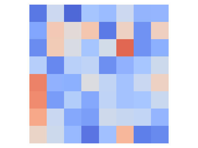


Directly comparing activation values does not work. Fig. 6 (a) and (b) show the average feature maps at the second last convolutional layer for the target class samples and the victim class samples stamped with the trigger, respectively, for the aforementioned trojaned model #7. Each block denotes the mean of the normalized activation values in a feature map. The L2 distance of the two is 0.59 as shown in the caption of (b). It measures the distance between the stamped samples and the clean target class samples. Ideally, a natural trigger would yield a small L2 distance as it possesses the target class features. Figures (c) and (d) show the corresponding information for a clean model, with the L2 distance 0.74 (larger than 0.59). Observe there is not a straightforward separation of the two. This is because such a simple method does not consider what features are critical. Empirical results can be found in Section 4.


trigger (L2:0.22)


trigger (L2:0.21)
A plausible improvement is to use attribution techniques to identify the important neuron/features and only compare their values. Fig. 7 (a) and (b) present the 10% most important neurons in the trojaned model #7 identified by an attribution technique DeepLift [67], for the target class samples and victim samples with the trigger, respectively. The L2 distance for the features in the intersection of the two (i.e., the features important in both) is 0.22 as shown in the caption of (b). Figures (c) and (d) show the information for the clean model #123 (with L2 distance 0.21). Even with the attribution method, the two are not that separable. This is because these techniques identify features that are important for a class or a sample whereas our technique identifies comparative importance, i.e., features that are important to distinguish two classes. The two are quite different as shown by the differences between Fig. 5 and Fig. 7. More results can be found in Section 4.
Applying a symmetric differential analysis similar to ours in the input space does not work well either. This is because semantic features/objects may appear in different positions of the inputs. Differencing pixels without aligning corresponding features/objects likely yields meaningless results.
3 Design
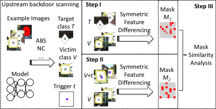
Fig. 8 shows the overview of Ex-Ray. The key component is the symmetric featuring differencing analysis. Given two sets of inputs, it identifies features of comparative importance, i.e., distinguishing the two sets. We also call them differential features or a mask for simplicity. Given a trigger generated by some upstream scanning technique (not our contribution) that flips class samples to class . In step I, the technique computes the mask separating and . In step II, it computes the mask separating and + samples, which are classified to . In step III, a similarity analysis is used to compare the two masks to determine if the trigger is natural. Next we will explain the components in details.
3.1 Symmetric Feature Differencing
Given two sets of inputs of classes and , respectively, and a hidden layer , the analysis identifies a smallest set of features/neurons (or mask) such that if we copy the values of from samples to samples, we can flip the samples to class , and vice versa. Note that such a set must exist as in the worse case, it is just the entire set of features at . We hence use optimization to find the smallest set.

Differencing Two Inputs. For explanation simplicity, we first discuss how the technique works on two inputs: in and in . We then expand it to compare two sets.
Let be a feed forward neural network under analysis. Given the inner layer , let be the sub-model up to layer and the sub-model after . Thus, . Let the number of features/neurons at be . The set of differential features (or mask) is denoted as an element vector with values in . means that the th neuron is not a differential feature; means is a must-differential feature; and means is a may-differential feature. The must and may features function differently during value copying, which will be illustrated later. Let be the negation of the mask such that with . The aforementioned symmetric property is hence denoted as follows.
| (1) |
| (2) |
Intuitively, when , the original th feature map is retained; when , the th feature map is replaced with that from the other sample; when , the feature map is the weighted sum of the th feature maps of the two samples. The reasoning is symmetric because the differences between two samples is a symmetric relation.
Example. Figure 9 illustrates an example of symmetric feature differencing. The box on the left shows the function and that on the right the function. The top row in the left box shows that five feature maps (in yellow) are generated by for a victim class sample . The bottom row shows that the five feature maps (in blue) for a target class sample . The box in the middle illustrates the symmetric differencing process. As suggested by the red entries in the mask in the middle (i.e., ), in the top row, the 3rd and 5th (yellow) feature maps are replaced with the corresponding (blue) feature maps from the bottom. Symmetric replacements happen in the bottom row as well. On the right, the mutated feature maps flip the classification results to and to , respectively.
Generating Minimal Mask by Optimization. The optimization to find the minimal is hence the following.
| (3) | ||||
To solve this optimization problem, we devise a loss in (4). It has three parts. The first part is to minimize the mask size. The second part is a barrier loss for constraint (1), with the cross entropy loss when replacing ’s features. Coefficients is dynamic. When the cross entropy loss is larger than a threshold , is set to a large value . This forces to satisfy constraint (1). When the loss is small indicating the constraint is satisfied, is changed to a small value . The optimization hence focuses on minimizing the mask. The third part is similar.
| (4) | ||||
Differencing Two Sets. The algorithm to identify the differential features of two sets can be built from the primitive of comparing two inputs. Given two sets of class and of class , ideally the mask should satisfy the constraints (1) and (2) for any and . While such a mask must exist (with the worst case containing all the features), minimizing it becomes very costly. Assume . The number of constraints that need to be satisfied during optimization is . Therefore, we develop a stochastic method that is . Specifically, let and be random orders of and , respectively. We minimize such that it satisfies constraints (1) and (2) for all pairs (, ), with . Intuitively, we optimize on a set of random pairs from and that cover all the individual samples in and . The loss function is hence the following.
When and have one-to-one mapping, such as the victim class samples and their compromised versions that have the trigger embedded, we can directly use the mapping in optimization instead of a random mapping. We use Adam optimizer [40] with a learning rate 5e-2 and 400 epochs. Masks are initialized to all 1 to begin with. This denotes a conservative start since such masks suggest swapping all feature maps, which must induce the intended classification results swap.
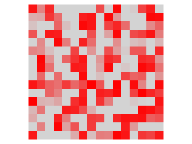
Example. Figure 10 shows how masks change over time for a benign model #4 from TrojAI round 2. Figure (a) shows the target class and (f) the victim class with a trigger generated by ABS (close to the center resembling the symbol in the middle of target class). Observe that the two classes are similar and hence ABS generates a small trigger that can flip to . Figures (b)-(e) show the changes of mask between and +trigger and (g)-(j) for the mask between and . Observe that in both cases, the initially all-1 masks (i.e., all red) are reduced to having sparse 1’s and some smaller-than-1 values. The masks in the top row consistently share substantial commonality with those in the bottom row, suggesting the similarity of the differential features.


Symmetry Is Necessary. Observe that our technique is symmetric. Such symmetry is critical to effectiveness. One may wonder that a one-sided analysis that only enforces constraint (2) may be sufficient. That is, is the minimal set of features that when copied from (target) samples to (victim) samples can flip the samples to class . However, this is insufficient. In many cases, misclassfication (of a sample to ) can be induced when strong features of class are suppressed (instead of adding strong features). Such features cannot be identified by the aforementioned one-sided analysis, while they can be identified by the analysis along the opposite direction (i.e., constraint (1)). Our experiments in Section 4 show the importance of symmetry.
Example. Fig. 11 presents an example for one-sided masks from a clean model #18 in TrojAI round 3. Figures (a) and (b) present the victim and target classes and (c) a natural trigger generated by ABS, which resembles the central symbol in the target class. Figure (d) shows the one-sided mask from to , meaning that copying/mixing the feature maps as indicated by the mask from samples to samples can flip the classification results to . Figure (e) shows the one-sided mask from to +trigger. Note that +trigger samples are classified to . Although in both cases samples are flipped to , the two one-sided masks have only one entry in common, suggesting that the ways they induce the classification results are different. In contrast, the symmetric masks (not shown due to space limitations) share a lot of commonality.


3.2 Comparing Differential Feature Sets To Identify Natural Backdoors
As shown in Fig. 8, we first compute the differential features between the victim and target classes, denoted as , and then those between the victim samples and their compromised versions, denoted as . Next, we explain how to compare and to determine if the trigger is natural. Intuitively and should share a lot of commonality when the trigger is natural, as reflected in the following condition.
| (5) | ||||
In (5), yields a vector whose elements are the minimal between the corresponding elements in and . It essentially represents the intersection of the two masks. The hyperparameter stands for a threshold to distinguish natural and injected triggers. Intuitively, the condition asserts that if the size of mask intersection is larger than times the minimum size of the two masks, meaning the two have a large part in common, the trigger is natural. If all the reverse engineered triggers for a model are natural, the model is considered clean.
Additional Validation Checks. In practice, due to the uncertainty in the stochastic symmetric differencing algorithm, the presence of local minimums in optimization, and the small number of available clean samples, and may not have a lot in common. However, they should nonetheless satisfy the semantic constraint that both should denote natural feature differences of the victim and target classes if the trigger is natural. Therefore, we propose an additional cross-validation check that tests if functionally and can take each other’s place in satisfying constraints (1) and (2). In particular, while is derived by comparing the victim class and the target class clean samples, we copy the feature maps indicated by between the victim samples and their compromised versions with trigger and check if the intended class flipping can be induced; similarly, while is derived by comparing the victim class samples and their compromised versions, we copy the feature maps indicated by between the victim clean samples and the target clean samples to see if the intended class flipping can be induced. If so, the two are functionally similar and the trigger is natural. The check is formulated as follows.
| (6) | ||||
Here, is a function to evaluate prediction accuracy on a set of samples and a threshold (0.8 in the paper). We use to denote applying on each sample in for representation simplicity.
4 Evaluation
Ex-Ray is implemented on PyTorch [58]. We will release the code upon publication. We conduct a number of experiments, including evaluating Ex-Ray on TrojAI rounds 2-4 datasets (with round 4 the latest) and a number of ImageNet pre-trained and trojaned models. We also apply Ex-Ray to detect composite backdoors and reflection backdoors in models for CIFAR10, and hidden-trigger backdoors in models for ImageNet. These are semantic backdoors, meaning that their triggers are natural objects/features instead of noise-like patches/watermarks. They may be large and complex. We study the performance of Ex-Ray in different settings, and compare with 8 baselines that make use of simple L2 distance, attribution/interpretation techniques, and one-sided (instead of symmetric) analysis. At the end, we design an adaptive attack and evaluate Ex-Ray against it.
Datasets, Models and Hyperparameter Setting. Note that the data processed by Ex-Ray are trained models. We use TrojAI rounds 2-4 training and test datasets [4]. Ex-Ray does not require training and hence we use both training and test sets as regular datasets in our experiments. TrajAI round 2 training set has 552 clean models and 552 trojaned models with 22 structures. It has two types of backdoors: polygons and Instagram filters. Round 2 test set has 72 clean and 72 trojaned models. Most performers had difficulties for round 2 due to the prevalence of natural triggers. IARPA hence introduced adversarial training [54, 82] in round 3 to enlarge the distance between classes and suppress natural triggers. Round 3 training set has 504 clean and 504 trojaned models and the test set has 144 clean and 144 trojaned models. In round 4, triggers may be position dependent, meaning that they only cause misclassification when stamped at a specific position inside the foreground object. A model may have multiple backdoors. The number of clean images provided is reduced from 10-20 (in rounds 2 and 3) to 2-5. Its training set has 504 clean and 504 trojaned models and the test set has 144 clean and 144 trojaned models. Training sets were evaluated on our local server whereas test set evaluation was done remotely by IARPA on their server. At the time of evaluation, the ground truth of test set models was unknown.
We also use a number of models on ImageNet. They have the VGG, ResNet and DenseNet structures. We use 7 trojaned models from [48] and 17 pre-trained clean models from torchvision zoo [3]. In the composite attack experiment, we use 25 models on CIFAR10. They have the Network in Network structure. Five of them are trojaned (by composite backdoors) using the code provided at [46]. We further mix them with 20 pre-trained models from [48]. In the reflection attack experiment, we use 25 Network in Network models on CIFAR10. Five of them are trojaned (by reflection backdoors) using the code provided at [50]. The 20 pre-trained clean models are from [48]. In the hidden trigger attack experiment, we use 23 models on ImageNet. Six of them are trojaned with hidden-triggers using the code at [64] and they are mixed with 17 pre-trained clean models from torchvision zoo [3].
The other settings can be found in Appendix A.
4.1 Experiments on TrojAI and ImageNet Models
| TrojAI R2 | TrojAI R3 | TrojAI R4 | ImageNet | ||||||||||||||||||||||||||||||||||||||
|
|
|
|
|
|
|
|||||||||||||||||||||||||||||||||||
| TP | FP | Acc | TP | FP | Acc | TP | FP | Acc | TP | FP | Acc | TP | FP | Acc | TP | FP | Acc | TP | FP | Acc | |||||||||||||||||||||
| Vanilla ABS | 254 | 218 | 0.710 | 260 | 293 | 0.626 | 235 | 208 | 0.702 | 213 | 334 | 0.528 | 137 | 355 | 0.442 | 331 | 376 | 0.531 | 7 | 7 | 0.708 | ||||||||||||||||||||
| Inner L2 | 188 | 93 | 0.782 | 153 | 123 | 0.703 | 210 | 111 | 0.798 | 133 | 123 | 0.680 | 73 | 137 | 0.680 | 208 | 217 | 0.572 | 7 | 0 | 1 | ||||||||||||||||||||
| Inner RF | 192 | 76 | 0.807 | 196 | 101 | 0.781 | 159 | 46 | 0.816 | 153 | 110 | 0.724 | 133 | 265 | 0.575 | 330 | 353 | 0.556 | 7 | 0 | 1 | ||||||||||||||||||||
| IG | 172 | 29 | 0.840 | 192 | 66 | 0.818 | 162 | 58 | 0.804 | 52 | 41 | 0.681 | 84 | 53 | 0.827 | 210 | 87 | 0.725 | 5 | 0 | 0.917 | ||||||||||||||||||||
| Deeplift | 152 | 11 | 0.837 | 189 | 21 | 0.869 | 162 | 59 | 0.803 | 78 | 67 | 0.681 | 84 | 54 | 0.825 | 203 | 54 | 0.755 | 6 | 0 | 0.958 | ||||||||||||||||||||
| Occulation | 173 | 24 | 0.847 | 207 | 47 | 0.860 | 164 | 58 | 0.807 | 78 | 66 | 0.683 | 85 | 52 | 0.830 | 251 | 107 | 0.749 | 7 | 3 | 0.875 | ||||||||||||||||||||
| NE | 180 | 58 | 0.814 | - | - | - | 187 | 72 | 0.819 | - | - | - | 59 | 72 | 0.759 | - | - | - | 7 | 4 | 0.833 | ||||||||||||||||||||
| 1-sided(V to T) | 157 | 19 | 0.833 | 195 | 33 | 0.862 | 202 | 62 | 0.852 | 153 | 51 | 0.802 | 107 | 82 | 0.818 | 236 | 50 | 0.798 | 7 | 0 | 1 | ||||||||||||||||||||
| 1-sided(T to V) | 134 | 4 | 0.824 | 158 | 18 | 0.835 | 187 | 50 | 0.848 | 134 | 27 | 0.808 | 102 | 56 | 0.850 | 179 | 9 | 0.779 | 1 | 1 | 0.958 | ||||||||||||||||||||
| Ex-Ray | 198 | 19 | 0.883 | 204 | 32 | 0.874 | 200 | 46 | 0.870 | 149 | 39 | 0.812 | 105 | 53 | 0.859 | 242 | 46 | 0.809 | 7 | 0 | 1 | ||||||||||||||||||||
In the first experiment, we evaluate Ex-Ray on TrojAI rounds 2-4 training sets and the ImageNet models. We do not include TrojAI test sets in this experiment as the test sets are hosted on an IARPA server and do not provide ground-truth information. One can only submit a solution to the server, which returns the overall scanning accuracy and cross-entropy loss. Here we use ABS as the upstream scanner as it is much faster than NC.
A critical setup for scanners that produce triggers, such as ABS and NC, is the maximum trigger size. A large value enables detecting injected backdoors with large triggers, while producing a lot of natural triggers and hence false positives. Fig. 12 studies how the true positives (TPs) and false positives (FPs) change with different trigger bounds in ABS, on the TrojAI rounds 2-4 training sets. Observe that both grow with the trigger size. Observe that there is a lower FP rate in round 3 (compared to round 2), illustrating the effect of adversarial training, although the number is still large when the trigger size is large. Round 4 has the highest FP rate because the number of clean images available is decreased and it is hence very easy for scanners to find (bogus) triggers that can induce misclassification on all the available images.
Based on the study, we use the trigger size bound 900 pixels for round 2, 1600 pixels for round 3, and 1200 pixels for round 4 for our experiment such that the upstream scanner does not miss many true positives to begin with and we can stress test Ex-Ray.

Baselines. In the experiment, we compare Ex-Ray against 8 baselines. The first baseline is using L2 distance of inner activation between and . Such a distance for a natural trigger is supposed to be smaller than that of an injected trigger (more in Section 2). We use unsupervised learning to report the best separation. In the second baseline, we use half of the models to train a random forest classifier based on the inner activations and logits values to distinguish natural and injected triggers and test it on the other half. Specifically, the classifier takes the L2 distance between and , L2 distance between and , L2 distance between and , logits of , logits of and logits of . The third baseline uses integrated gradients (IG) [70], an attribution technique, to find important neurons for and for and then apply the aforementioned L2 distance comparison on the 10% most important neurons (more in Section 2). Originally, integrated gradients were used in model explanation and identify important pixels. We adapt it to work on inner layers and identify important neurons. The next three baselines are similar to the third except having different methods to identify important neurons. Specifically, the fourth baseline uses Deeplift [67], the fifth uses Occlusion [7] and the sixth uses Network Dissection (NE) [12]. For baselines 4-7, we use unsupervised learning to find the best separation (of natural and injected backdoors). We will release the settings together with our system upon publication. Ex-Ray is symmetric. To study the necessity of symmetry, the seventh and eighth baselines are one-sided versions of Ex-Ray, that is, requiring satisfying either constraint (1) or (2) in Section 3.
The results are shown in Table 1. The first column shows the methods. The first method is the vanilla ABS. Columns 2-4 show the results for TrojAI round 2 models with polygon backdoors. Column 2 shows the number of true positives (TPs). Note that there are 276 trojaned models with polygon backdoors. As such the vanilla ABS having 254 TPs means it has 22 false negatives. Column 3 shows the number of false positives (FPs) out of the 552 clean models. Column 4 shows the overall detection accuracy (on the total 552+276=828 models). Columns 5-7 show the results for round 2 models with Instagram filter backdoors. ABS uses a different method for filter backdoors. Instead of reverse engineering a pixel patch, it reverse engineers a one-layer kernel denoting general filter transformation [48]. Hence, we separate the evaluation of Ex-Ray on the two kinds of backdoors. Note that the accuracy is computed considering the same 552 clean models. The overall results (for all kinds of backdoors) on the leaderboard are presented later. Columns 8-13 show the results for round 3 and columns 14-19 for round 4. Columns 14-16 show the results for ImageNet patch attack.
| Round 2 | Round 3 | Round 4 | ||||||
| CE loss | ROC-AUC | CE loss | ROC-AUC | CE loss | ROC-AUC | |||
| ABS only | 0.685 | 0.736 | 0.541 | 0.822 | 0.894 | 0.549 | ||
| ABS+Ex-Ray | 0.324 | 0.892 | 0.323 | 0.9 | 0.322 | 0.902 | ||
| Deficit from top | 0 | 0 | 0.023 | -0.012 | 0 | 0 | ||
The results show that the vanilla ABS has a lot of FPs (in order not to lose TPs) and Ex-Ray can substantially reduce the FPs by 78-100% with the cost of increased FNs (i.e., losing TPs) by 0-30%. The overall detection accuracy improvement (from vanilla ABS) is 17-41% across the datasets. Also observe that Ex-Ray consistently outperforms all the baselines, especially the non-Ex-Ray ones. Attribution techniques can remove a lot of natural triggers indicated by the decrease of FPs. However, they preclude many injected triggers (TPs) as well, leading to inferior performance. The missing entries for NE are because it requires an input region to decide important neurons, rendering it inapplicable to filters that are pervasive. Symmetric Ex-Ray outperforms the one-sided versions, suggesting the need of symmetry.
Results on TrojAI Leaderboard (Test Sets). In the first experiment, we evaluate Ex-Ray in a most challenging setting, which causes the upstream scanner to produce the largest number of natural triggers (and also the largest number of true injected triggers). TrojAI allows performers to tune hyperparameters based on the training sets. We hence fine-tune our ABS+Ex-Ray pipeline, searching for the best hyperparameter settings such as maximum trigger size, optimization epochs, , , and , on the training sets and then evaluate the tuned version on the test sets. Table 2 shows the results. In two of the three rounds, our solution achieved the top performance666TrojAI ranks solutions based on the cross-entropy loss of scanning results. Intuitively, the loss increases when the model classification diverges from the ground truth. Smaller loss suggests better performance [4]. Past leaderboard results can be found at [5]. . In round 3, it ranked number 2 and the results are comparable to the top performer. In addition, it beat the IARPA round goal (i.e., cross-entry loss lower than 0.3465 ) for all the three rounds. We also want to point out that Ex-Ray is not a stand-alone defense technique. Hence, we do not directly compare with existing end-to-end defense solutions. Our performance on the leaderboard, especially for round 2 that has a large number of natural backdoors and hence caused substantial difficulties for most performers777Most performers had lower than 0.80 accuracy in round 2., suggests the contributions of Ex-Ray. As far as we know, many existing solutions such as [48, 77, 41, 71, 69, 24, 38, 17, 68] have been tested in the competition by different performers.
Runtime. On average, Ex-Ray takes 12s to process a trigger, 95s to process a model. ABS takes 337s to process a model, producing 8.5 triggers on average.
Effects of Hyperparameters. We study Ex-Ray performance with various settings, including the different layer to which Ex-Ray is applied, different trigger size settings (in the upstream scanner) and different SSIM score bound (in the upstream filter backdoor scanning to ensure the generated kernel does not over-transform an input), and the , , and settings of Ex-Ray. The results are in Appendix B. They show that Ex-Ray is reasonably stable with various settings.
| Vanilla | +Ex-Ray | |||||||||||
|---|---|---|---|---|---|---|---|---|---|---|---|---|
| TP | T | FP | C | Acc | TP | T | FP | C | Acc | Acc Inc | ||
| NC | 180 | 252 | 332 | 552 | 0.483 | 127 | 252 | 73 | 552 | 0.732 | 0.249 | |
| SRI-RE | 164 | 252 | 272 | 552 | 0.536 | 112 | 252 | 97 | 552 | 0.685 | 0.149 | |
| SRI-CLS | 120 | 146 | 17 | 158 | 0.858 | 119 | 146 | 9 | 158 | 0.882 | 0.024 | |
4.2 Using Ex-Ray with Different Upstream Scanners
In this experiment, we use Ex-Ray with different upstream scanners, including Neural Cleanse (NC) [77] and the Bottom-pp-Top-down method by the SRI team in the TrojAI competition [1]. The latter has two sub-components, trigger generation and a classifier that makes use of features collected from the trigger generation process. We created two scanners out of their solution. In the first one, we apply Ex-Ray on top of their final classification results (i.e., using Ex-Ray as a refinement). We call it SRI-CLS. In the second one, we apply Ex-Ray right after their trigger generation. We have to replace their classifier with the simpler unsupervised learning (i.e., finding the best separation) as adding Ex-Ray changes the features and nullifies their original classifier. We call it SRI-RE. We use the round 2 clean models and models with polygon triggers to conduct the study as NC does not handle Instagram filter triggers. For SRI-CLS, the training was on 800 randomly selected models and testing was on the remaining 146 trojaned models and 158 clean models. The other scanners do not require training. The results are shown in Table 3. The T and C columns stand for the number of trojaned and clean models used in testing, respectively. Observe that the vanilla NC identifies 180 TPs and 332 FPs with the accuracy of 44.7%. With Ex-Ray, the FPs are reduced to 73 (81.1% reduction) and the TPs become 127 (29.4% degradation). The overall accuracy improves from 44.7% to 70.8%. The improvement for SRI-RE is from 53.6% to 68.5%. The improvement for SRI-CLS is relative less significant. That is because 0.882 accuracy is already very close to the best performance for this round. The results show that Ex-Ray can consistently improve upstream scanner performance. Note that the value of Ex-Ray lies in suppressing false warnings. It offers little help if the upstream scanner has substantial false negatives. In this case, users may want to tune the upstream scanner to have minimal false negatives and then rely on the downstream Ex-Ray to prune the resulted false positives like we did in the ABS+Ex-Ray pipeline.
4.3 Study of Failing Cases by Ex-Ray
According to Table 1, Ex-Ray cannot prune all the natural triggers (causing FPs) and it may mistakenly prune injected triggers (causing FNs). Here, we study two cases: one demonstrating why Ex-Ray fails to detect a natural trigger and the other demonstrating why Ex-Ray misclassifies an injected trigger to natural. Fig. 13 shows a clean model with a natural trigger but Ex-Ray fails to prune it, with (a) and (b) the victim and target classes, respectively, and (c) the natural trigger by ABS. Observe that the victim and target classes are really close. Even the central symbols look similar. As such, small and arbitrary input perturbations as those in (c) may be sufficient to induce misclassification. Such perturbations may not resemble any of the distinguishing features between the two classes at all, rendering Ex-Ray ineffective. Fig. 14 shows a trojaned model that Ex-Ray considers clean, with (a) and (b) the victim class with the injected trigger (ground truth provided by IARPA) and the target class, respectively, and (c) the trigger generated by ABS. Observe that a strong distinguishing feature of the victim and target classes is the red versus the white borders. The injected trigger happens to be a red polygon, which shares a lot of commonality with the differential features of the classes, rendering Ex-Ray ineffective.


4.4 Detecting Semantic Backdoor Attacks
While early backdoor attacks on image classifiers used noise-like pixel patches/watermarks that are small, recent backdoor attacks showed that models can be trojaned with natural objects and features that may be large and complex. As such, scanners that generate small triggers to determine if a model has backdoor become ineffective. A possible solution is to enlarge the size bound such that the injected large triggers can be generated. However, this entails a lot of false positives as it admits many natural triggers. In this experiment, we show that by enlarging the trigger bound of ABS and using Ex-Ray to prune false positives, we can detect composite backdoors [46], hidden-trigger backdoors [64], and reflection backdoors [50].
Detecting Composite Backdoor. Composite backdoor uses composition of existing benign features as triggers (see Fig. 4 in Section 1). The experiment is on 5 models trojaned by the attack and 20 clean models on CIFAR10. We set the trigger size to 600 pixels in order to reverse engineer the large trigger features used in the attack. In Table 4, our results show that we can achieve 0.84 accuracy (improved from 0.2 by vanilla ABS), reducing the false positives from 20 to 4. It shows the potential of Ex-Ray.
Fig. 15 shows a natural trigger and an injected composite trigger. Figures (a) and (b) show a natural trigger (generated by ABS) with the target label dog and a sample from the dog class (in CIAFR10), respectively. Observe that the trigger has a lot of dog features (and hence pruned by Ex-Ray). Figures (c) and (d) show a composite trigger used during poisoning, which is a combination of car and airplane, and the trigger generated by ABS, respectively. Figure (e) shows the target label bird. Observe that the reverse engineered trigger has car features (e.g., wheels). Ex-Ray recognizes it as an injected trigger since it shares very few features with the bird class.


| TP | FP | FN | TN | Acc | |
|---|---|---|---|---|---|
| ABS | 5 | 20 | 0 | 0 | 0.2 |
| ABS+Ex-Ray | 5 | 4 | 0 | 16 | 0.84 |


| TP | FP | FN | TN | Acc | |
|---|---|---|---|---|---|
| ABS | 5 | 17 | 0 | 3 | 0.32 |
| ABS+Ex-Ray | 5 | 3 | 0 | 17 | 0.88 |
Detecting Reflection Backdoor. Reflection may occur when taking picture behind a glass window. Reflection backdoors uses the reflection of an image as the trojan trigger. Figure 16 (a) and (b) shows an image of triangle sign and its reflection on an image of airplane. Reflection attack uses the reflection of a whole image as the trigger, which is large and complex. We evaluate ABS+Ex-Ray on 5 models trojaned with reflection backdoors and 20 clean models on CIFAR10. The trigger size bound is set to 256 (very large for CIFAR images). Table 5 shows that we can achieve 0.88 accuracy (improved from 0.32 by ABS), reducing the false positives from 17 to 3.
Figure 16 (c) and (d) show a natural trigger (generated by ABS) with the target label deer and a sample from the deer class. Observe that the trigger resembles deer antlers. Figure 16 (e) and (f) show the trigger generated by ABS with the target class airplane. Observe that the generated trigger has (triangle) features of the real trigger shown in Figure 16 (a) and (b). Ex-Ray classifies it as injected as it shares few features with airplane (Figure 16 (f)).
Detecting Hidden-trigger Backdoor. Hidden-trigger attack does not directly use trigger to poison training data. Instead, it introduces perturbation on the images of target label such that the perturbed images induce similar inner layer activations to the images of victim label stamped with the trigger. Since the inner layer activations represent features, the model picks up the correlations between trigger features and the target label. Thus images stamped with the trigger are misclassified to the target label at test time. The attack is a clean label attack. Since the trigger is not explicit, the attack is more stealthy compared to data poisoning. On the other hand, the trojaning process is more difficult, demanding larger triggers, causing problems for existing scanners. For example, it requires the trigger size to be 6060 for ImageNet to achieve a high attack success rate. Figure 17 (a) and (b) show a trigger and an ImageNet sample stamped with the trigger, with the target label terrier dog shown in (f).
We evaluate ABS+Ex-Ray on 6 models trojaned with hidden-triggers and 17 clean models on ImageNet. The trigger size bound for ABS is set to 4000. Table 6 shows that we can achieve 0.82 accuracy (improved from 0.3 by ABS), reducing the number of false positives from 16 to 3. Figure 17 (c) and (d) show a natural trigger generated by ABS and its target label Jeans. Observe that the center part of natural trigger resembles a pair of jeans pants. Since the natural trigger mainly contains features of the target label, it is pruned by Ex-Ray. Figure 17 (e) shows the generated trigger by ABS for the target label (f). The trigger has few in common with the target label and thus is classified as injected by Ex-Ray.
| TP | FP | FN | TN | Acc | |
|---|---|---|---|---|---|
| ABS | 6 | 16 | 0 | 1 | 0.30 |
| ABS+Ex-Ray | 5 | 3 | 1 | 14 | 0.82 |


| Weight of adaptive loss | 1 | 10 | 100 | 1000 | 10000 |
|---|---|---|---|---|---|
| Acc | 0.89 | 0.88 | 0.87 | 0.82 | 0.1 |
| Asr | 0.99 | 0.99 | 0.99 | 0.97 | - |
| FP/ # of clean models | 0 | 0.2 | 0.2 | 0.65 | - |
| TP/ # of trojaned models | 1 | 1 | 1 | 1 | - |
4.5 Adaptive Attack
Ex-Ray is part of a defense technique and hence vulnerable to adaptive attack. We devise an adaptive attack that forces the internal activations of victim class inputs embedding the trigger to resemble the activations of the clean target class inputs such that Ex-Ray cannot distinguish the two. In particular, we train a Network in Network model on CIFAR10 with a given 88 patch as the trigger. In order to force the inner activations of images stamped with the trigger to resemble those of target class images, we design an adaptive loss which is to minimize the differences between the two. In particular, we measure the differences of the means and standard deviations of feature maps. During training, we add the adaptive loss to the normal cross-entropy loss. The effect of adaptive loss is controlled by a weight value, which essentially controls the strength of attack as well. Besides the adaptively trojaned model, we also train 20 clean models on CIFAR10 to see if ABS+Ex-Ray can distinguish the trojaned and clean models.
The results are shown in Table 7. The first row shows the adaptive loss weight. A larger weight value indicates stronger attack. The second row shows the trojaned model’s accuracy on clean images. The third row shows the attack success rate of the trojaned model. The fourth row shows the FP rate. The fifth row shows the TP rate. Observe while ABS+Ex-Ray does not miss trojaned models, its FP rate grows with the strength of attack. When the weight value is 1000, the FP rate becomes 0.65, meaning Ex-Ray is no longer effective. However, the model accuracy also degrades a lot in this case.
4.6 Fixing Models with Injected and Natural Backdoors
As mentioned in Section 1, an important difference between injected and natural backdoors is that the latter is inevitable and difficult to fix. To make the comparison, we try to fix 5 benign models and 5 trojaned models on CIFAR10. The trojaned models are trojaned by label-specific data poisoning. Here we use unlearning [77] which stamps triggers generated by scanning methods on images of victim label to finetune the model and forces the model to unlearn the correlations between the triggers and the target label. The process is iterative, bounded by the level of model accuracy degradation. The level of repair achieved is measured by the trigger sizes of the fixed model. Larger triggers indicate the corresponding backdoors become more difficult to exploit. The trigger size increase rate suggests the difficulty level of repair.
Table 8 shows the average accuracy and average reverse engineered trigger size before and after fixing the models. All models have the same repair budget. We can see that natural triggers have a larger accuracy decrease. Natural trigger size only increases by 34.4 whereas injected trigger size increases by 78, supporting our hypothesis. More detailed results can be found in Appendix C. Note that model repair is not the focus of the paper and trigger size may not be a good metric to evaluate repair success for the more complex semantic backdoors. The experiment is to provide initial insights. A thorough model repair solution belongs to our future work.
| Natural Trigger | Injected Trigger | ||||
|---|---|---|---|---|---|
| Before | After | Before | After | ||
| Avg Acc | 88.7% | 85.9% | 86.4% | 85.4% | |
| Avg Trigger Size | 25.8 | 60.2 | 19 | 97 | |
5 Related Work
Backdoor Attack. Data poisoning [32, 19] injects backdoor by changing the label of inputs with trigger. Clean label attack [66, 94, 74, 92, 64] injects backdoor without changing the data label. Bit flipping attack [62, 61] proposes to trojan models by flipping weight value bits. Dynamic backdoor [65, 56] focuses on crafting different triggers for different inputs and breaks the defense’s assumption that trigger is universal. Ren et al. [57] proposed to combine adversarial example generation and model poisoning to improve the effectiveness of both attacks. There are also attacks on NLP tasks [90, 18, 42], Graph Neural Network [91, 83], transfer learning [63, 78, 86], and federated learning [84, 79, 72, 10, 25]. Ex-Ray is a general primitive that may be of use in defending these attacks.
Backdoor Attack Defense. ULP [41] trains a few universal input patterns and a classifier from thousands of benign and trojaned models. The classifier predicts if a model has backdoor based on activations of the patterns. Xu et al. [85] proposed to detect backdoor using a meta classifier trained on a set of trojaned and benign models. Qiao et al. [60] proposed to reverse engineer the distribution of triggers. Hunag et al. [35] found that trojaned and clean models react differently to input perturbations. Cassandra [89] and TND [80] found that universal adversarial examples behave differently on trojaned and clean models and used this observation to detect backdoor. TABOR [33] and NeuronInspect [36] used an AI explanation technique to detect backdoor. NNoculation [75] used broad spectrum random perturbations and GAN based techniques to reverse engineer trigger. Besides backdoor detection, there are techniques aiming at removing backdoor. Fine-prune [47] removed backdoors by pruning out compromised neurons. Borgnia et al. [13] and Zeng et al. [88] proposed to use data augmentation technique to mitigate backdoor effect. Wang et al. [76] proposed to use randomized smoothing to certify robustness against backdoor attacks. There are techniques that defend backdoor attacks by data sanitization where they prune out poisoned training inputs [14, 37, 55, 59]. There are also techniques that detect if a given input is stamped with trigger [53, 71, 29, 16, 45, 52, 20, 73, 27, 15, 23, 75]. They target a different problem as they require inputs with embedded triggers. Ex-Ray is orthogonal to most of these techniques and can serve as a performance booster. Excellent surveys of backdoor attack and defense can be found at [44, 51, 28, 43].
Interpretation/Attribution. Ex-Ray is also related to model interpretation and attribution, e.g., those identifying important neurons and features [70, 67, 7, 12, 6, 67, 8, 21, 22, 26, 93, 11, 34, 31, 87]. The differences lie in that Ex-Ray focuses on finding distinguishing features of two classes. Exiting work [39] utilizes random examples and training samples of a class (e.g., zebra) to measure the importance of a concept (e.g., ‘striped’) for the class. It however does not find distinguishing internal features.
6 Conclusion
We develop a method to distinguish natural and injected backdoors. It is built on a novel symmetric feature differencing technique that identifies a smallest set of features separating two sets of samples. Our results show that the technique is highly effective and enabled us to achieve top results on the rounds 2 and 4 leaderboard of the TrojAI competition, and rank the 2nd in round 3. It also shows potential in handling complex and composite semantic-backdoors.
References
- [1] Github - sri-csl/trinity-trojai: This repository contains code developed by the sri team for the iarpa/trojai program. https://github.com/SRI-CSL/Trinity-TrojAI.
- [2] Keras applications. https://keras.io/api/applications/.
- [3] torchvision.models — pytorch 1.7.0 documentation. https://pytorch.org/docs/stable/torchvision/models.html.
- [4] Trojai leaderboard. https://pages.nist.gov/trojai/.
- [5] Trojai past leaderboards. https://pages.nist.gov/trojai/docs/results.html#previous-leaderboards.
- [6] Marco Ancona, Enea Ceolini, Cengiz Öztireli, and Markus Gross. Towards better understanding of gradient-based attribution methods for deep neural networks. arXiv preprint arXiv:1711.06104, 2017.
- [7] Marco Ancona, Enea Ceolini, Cengiz Öztireli, and Markus Gross. Towards better understanding of gradient-based attribution methods for deep neural networks. In International Conference on Learning Representations, 2018.
- [8] Sebastian Bach, Alexander Binder, Grégoire Montavon, Frederick Klauschen, Klaus-Robert Müller, and Wojciech Samek. On pixel-wise explanations for non-linear classifier decisions by layer-wise relevance propagation. PloS one, 10(7):e0130140, 2015.
- [9] Eugene Bagdasaryan and Vitaly Shmatikov. Blind backdoors in deep learning models. arXiv preprint arXiv:2005.03823, 2020.
- [10] Eugene Bagdasaryan, Andreas Veit, Yiqing Hua, Deborah Estrin, and Vitaly Shmatikov. How to backdoor federated learning. In International Conference on Artificial Intelligence and Statistics, pages 2938–2948. PMLR, 2020.
- [11] Anthony Bau, Yonatan Belinkov, Hassan Sajjad, Nadir Durrani, Fahim Dalvi, and James Glass. Identifying and controlling important neurons in neural machine translation. arXiv preprint arXiv:1811.01157, 2018.
- [12] David Bau, Bolei Zhou, Aditya Khosla, Aude Oliva, and Antonio Torralba. Network dissection: Quantifying interpretability of deep visual representations. In Proceedings of the IEEE conference on computer vision and pattern recognition, pages 6541–6549, 2017.
- [13] Eitan Borgnia, Valeriia Cherepanova, Liam Fowl, Amin Ghiasi, Jonas Geiping, Micah Goldblum, Tom Goldstein, and Arjun Gupta. Strong data augmentation sanitizes poisoning and backdoor attacks without an accuracy tradeoff. arXiv preprint arXiv:2011.09527, 2020.
- [14] Yinzhi Cao, Alexander Fangxiao Yu, Andrew Aday, Eric Stahl, Jon Merwine, and Junfeng Yang. Efficient repair of polluted machine learning systems via causal unlearning. In Proceedings of the 2018 on Asia Conference on Computer and Communications Security, pages 735–747, 2018.
- [15] Alvin Chan and Yew-Soon Ong. Poison as a cure: Detecting & neutralizing variable-sized backdoor attacks in deep neural networks. arXiv preprint arXiv:1911.08040, 2019.
- [16] Bryant Chen, Wilka Carvalho, Nathalie Baracaldo, Heiko Ludwig, Benjamin Edwards, Taesung Lee, Ian Molloy, and Biplav Srivastava. Detecting backdoor attacks on deep neural networks by activation clustering. arXiv preprint arXiv:1811.03728, 2018.
- [17] Huili Chen, Cheng Fu, Jishen Zhao, and Farinaz Koushanfar. Deepinspect: A black-box trojan detection and mitigation framework for deep neural networks. In IJCAI, pages 4658–4664, 2019.
- [18] Xiaoyi Chen, Ahmed Salem, Michael Backes, Shiqing Ma, and Yang Zhang. Badnl: Backdoor attacks against nlp models. arXiv preprint arXiv:2006.01043, 2020.
- [19] Xinyun Chen, Chang Liu, Bo Li, Kimberly Lu, and Dawn Song. Targeted backdoor attacks on deep learning systems using data poisoning. arXiv preprint arXiv:1712.05526, 2017.
- [20] Edward Chou, Florian Tramer, and Giancarlo Pellegrino. Sentinet: Detecting localized universal attack against deep learning systems. IEEE SPW 2020, 2020.
- [21] Nilaksh Das, Haekyu Park, Zijie J Wang, Fred Hohman, Robert Firstman, Emily Rogers, and Duen Horng Chau. Massif: Interactive interpretation of adversarial attacks on deep learning. In Extended Abstracts of the 2020 CHI Conference on Human Factors in Computing Systems, pages 1–7, 2020.
- [22] Yinpeng Dong, Hang Su, Jun Zhu, and Fan Bao. Towards interpretable deep neural networks by leveraging adversarial examples. arXiv preprint arXiv:1708.05493, 2017.
- [23] Min Du, Ruoxi Jia, and Dawn Song. Robust anomaly detection and backdoor attack detection via differential privacy. In International Conference on Learning Representations, 2019.
- [24] N Benjamin Erichson, Dane Taylor, Qixuan Wu, and Michael W Mahoney. Noise-response analysis for rapid detection of backdoors in deep neural networks. arXiv preprint arXiv:2008.00123, 2020.
- [25] Minghong Fang, Xiaoyu Cao, Jinyuan Jia, and Neil Gong. Local model poisoning attacks to byzantine-robust federated learning. In 29th USENIX Security Symposium (USENIX Security 20), pages 1605–1622, 2020.
- [26] Ruth Fong and Andrea Vedaldi. Net2vec: Quantifying and explaining how concepts are encoded by filters in deep neural networks. In Proceedings of the IEEE conference on computer vision and pattern recognition, pages 8730–8738, 2018.
- [27] Hao Fu, Akshaj Kumar Veldanda, Prashanth Krishnamurthy, Siddharth Garg, and Farshad Khorrami. Detecting backdoors in neural networks using novel feature-based anomaly detection. arXiv preprint arXiv:2011.02526, 2020.
- [28] Yansong Gao, Bao Gia Doan, Zhi Zhang, Siqi Ma, Anmin Fu, Surya Nepal, and Hyoungshick Kim. Backdoor attacks and countermeasures on deep learning: A comprehensive review. arXiv preprint arXiv:2007.10760, 2020.
- [29] Yansong Gao, Change Xu, Derui Wang, Shiping Chen, Damith C Ranasinghe, and Surya Nepal. Strip: A defence against trojan attacks on deep neural networks. In Proceedings of the 35th Annual Computer Security Applications Conference, pages 113–125, 2019.
- [30] Andreas Geiger, Philip Lenz, Christoph Stiller, and Raquel Urtasun. Vision meets robotics: The kitti dataset. International Journal of Robotics Research (IJRR), 2013.
- [31] Amirata Ghorbani, James Wexler, James Y Zou, and Been Kim. Towards automatic concept-based explanations. In Advances in Neural Information Processing Systems, pages 9277–9286, 2019.
- [32] Tianyu Gu, Kang Liu, Brendan Dolan-Gavitt, and Siddharth Garg. Badnets: Evaluating backdooring attacks on deep neural networks. IEEE Access, 7:47230–47244, 2019.
- [33] Wenbo Guo, Lun Wang, Xinyu Xing, Min Du, and Dawn Song. Tabor: A highly accurate approach to inspecting and restoring trojan backdoors in ai systems. arXiv preprint arXiv:1908.01763, 2019.
- [34] Fred Hohman, Haekyu Park, Caleb Robinson, and Duen Horng Polo Chau. S ummit: Scaling deep learning interpretability by visualizing activation and attribution summarizations. IEEE transactions on visualization and computer graphics, 26(1):1096–1106, 2019.
- [35] Shanjiaoyang Huang, Weiqi Peng, Zhiwei Jia, and Zhuowen Tu. One-pixel signature: Characterizing cnn models for backdoor detection. arXiv preprint arXiv:2008.07711, 2020.
- [36] Xijie Huang, Moustafa Alzantot, and Mani Srivastava. Neuroninspect: Detecting backdoors in neural networks via output explanations. arXiv preprint arXiv:1911.07399, 2019.
- [37] Matthew Jagielski, Alina Oprea, Battista Biggio, Chang Liu, Cristina Nita-Rotaru, and Bo Li. Manipulating machine learning: Poisoning attacks and countermeasures for regression learning. In 2018 IEEE Symposium on Security and Privacy (SP), pages 19–35. IEEE, 2018.
- [38] Susmit Jha, Sunny Raj, Steven Fernandes, Sumit K Jha, Somesh Jha, Brian Jalaian, Gunjan Verma, and Ananthram Swami. Attribution-based confidence metric for deep neural networks. In Advances in Neural Information Processing Systems, pages 11826–11837, 2019.
- [39] Been Kim, Martin Wattenberg, Justin Gilmer, Carrie Cai, James Wexler, Fernanda Viegas, et al. Interpretability beyond feature attribution: Quantitative testing with concept activation vectors (tcav). In International conference on machine learning, pages 2668–2677. PMLR, 2018.
- [40] Diederik P Kingma and Jimmy Ba. Adam: A method for stochastic optimization. arXiv preprint arXiv:1412.6980, 2014.
- [41] Soheil Kolouri, Aniruddha Saha, Hamed Pirsiavash, and Heiko Hoffmann. Universal litmus patterns: Revealing backdoor attacks in cnns. In Proceedings of the IEEE/CVF Conference on Computer Vision and Pattern Recognition, pages 301–310, 2020.
- [42] Keita Kurita, Paul Michel, and Graham Neubig. Weight poisoning attacks on pre-trained models. arXiv preprint arXiv:2004.06660, 2020.
- [43] Shaofeng Li, Shiqing Ma, Minhui Xue, and Benjamin Zi Hao Zhao. Deep learning backdoors. arXiv preprint arXiv:2007.08273, 2020.
- [44] Yiming Li, Baoyuan Wu, Yong Jiang, Zhifeng Li, and Shu-Tao Xia. Backdoor learning: A survey. arXiv preprint arXiv:2007.08745, 2020.
- [45] Yiming Li, Tongqing Zhai, Baoyuan Wu, Yong Jiang, Zhifeng Li, and Shutao Xia. Rethinking the trigger of backdoor attack. arXiv preprint arXiv:2004.04692, 2020.
- [46] Junyu Lin, Lei Xu, Yingqi Liu, and Xiangyu Zhang. Composite backdoor attack for deep neural network by mixing existing benign features. In Proceedings of the 2020 ACM SIGSAC Conference on Computer and Communications Security, pages 113–131, 2020.
- [47] Kang Liu, Brendan Dolan-Gavitt, and Siddharth Garg. Fine-pruning: Defending against backdooring attacks on deep neural networks. In International Symposium on Research in Attacks, Intrusions, and Defenses, pages 273–294. Springer, 2018.
- [48] Yingqi Liu, Wen-Chuan Lee, Guanhong Tao, Shiqing Ma, Yousra Aafer, and Xiangyu Zhang. Abs: Scanning neural networks for back-doors by artificial brain stimulation. In Proceedings of the 2019 ACM SIGSAC Conference on Computer and Communications Security, pages 1265–1282, 2019.
- [49] Yingqi Liu, Shiqing Ma, Yousra Aafer, Wen-Chuan Lee, Juan Zhai, Weihang Wang, and Xiangyu Zhang. Trojaning attack on neural networks. In 25nd Annual Network and Distributed System Security Symposium, NDSS 2018, San Diego, California, USA, February 18-221, 2018. The Internet Society, 2018.
- [50] Yunfei Liu, Xingjun Ma, James Bailey, and Feng Lu. Reflection backdoor: A natural backdoor attack on deep neural networks. In European Conference on Computer Vision, pages 182–199. Springer, Cham, 2020.
- [51] Yuntao Liu, Ankit Mondal, Abhishek Chakraborty, Michael Zuzak, Nina Jacobsen, Daniel Xing, and Ankur Srivastava. A survey on neural trojans. IACR Cryptol. ePrint Arch., 2020:201, 2020.
- [52] Yuntao Liu, Yang Xie, and Ankur Srivastava. Neural trojans. In 2017 IEEE International Conference on Computer Design (ICCD), pages 45–48. IEEE, 2017.
- [53] Shiqing Ma and Yingqi Liu. Nic: Detecting adversarial samples with neural network invariant checking. In Proceedings of the 26th Network and Distributed System Security Symposium (NDSS 2019), 2019.
- [54] Aleksander Madry, Aleksandar Makelov, Ludwig Schmidt, Dimitris Tsipras, and Adrian Vladu. Towards deep learning models resistant to adversarial attacks. arXiv preprint arXiv:1706.06083, 2017.
- [55] Mehran Mozaffari-Kermani, Susmita Sur-Kolay, Anand Raghunathan, and Niraj K Jha. Systematic poisoning attacks on and defenses for machine learning in healthcare. IEEE journal of biomedical and health informatics, 19(6):1893–1905, 2014.
- [56] Tuan Anh Nguyen and Anh Tran. Input-aware dynamic backdoor attack. Advances in Neural Information Processing Systems, 33, 2020.
- [57] Ren Pang, Hua Shen, Xinyang Zhang, Shouling Ji, Yevgeniy Vorobeychik, Xiapu Luo, Alex Liu, and Ting Wang. A tale of evil twins: Adversarial inputs versus poisoned models. In Proceedings of the 2020 ACM SIGSAC Conference on Computer and Communications Security, pages 85–99, 2020.
- [58] Adam Paszke, Sam Gross, Soumith Chintala, Gregory Chanan, Edward Yang, Zachary DeVito, Zeming Lin, Alban Desmaison, Luca Antiga, and Adam Lerer. Automatic differentiation in pytorch. 2017.
- [59] Andrea Paudice, Luis Muñoz-González, and Emil C Lupu. Label sanitization against label flipping poisoning attacks. In Joint European Conference on Machine Learning and Knowledge Discovery in Databases, pages 5–15. Springer, 2018.
- [60] Ximing Qiao, Yukun Yang, and Hai Li. Defending neural backdoors via generative distribution modeling. In Advances in Neural Information Processing Systems, pages 14004–14013, 2019.
- [61] Adnan Siraj Rakin, Zhezhi He, and Deliang Fan. Bit-flip attack: Crushing neural network with progressive bit search. In Proceedings of the IEEE International Conference on Computer Vision, pages 1211–1220, 2019.
- [62] Adnan Siraj Rakin, Zhezhi He, and Deliang Fan. Tbt: Targeted neural network attack with bit trojan. In Proceedings of the IEEE/CVF Conference on Computer Vision and Pattern Recognition, pages 13198–13207, 2020.
- [63] Shahbaz Rezaei and Xin Liu. A target-agnostic attack on deep models: Exploiting security vulnerabilities of transfer learning. arXiv preprint arXiv:1904.04334, 2019.
- [64] Aniruddha Saha, Akshayvarun Subramanya, and Hamed Pirsiavash. Hidden trigger backdoor attacks. In Proceedings of the AAAI Conference on Artificial Intelligence, volume 34, pages 11957–11965, 2020.
- [65] Ahmed Salem, Rui Wen, Michael Backes, Shiqing Ma, and Yang Zhang. Dynamic backdoor attacks against machine learning models. arXiv preprint arXiv:2003.03675, 2020.
- [66] Ali Shafahi, W Ronny Huang, Mahyar Najibi, Octavian Suciu, Christoph Studer, Tudor Dumitras, and Tom Goldstein. Poison frogs! targeted clean-label poisoning attacks on neural networks. In Advances in Neural Information Processing Systems, pages 6103–6113, 2018.
- [67] Avanti Shrikumar, Peyton Greenside, Anna Shcherbina, and Anshul Kundaje. Not just a black box: Learning important features through propagating activation differences. arXiv preprint arXiv:1605.01713, 2016.
- [68] Karan Sikka, Indranil Sur, Susmit Jha, Anirban Roy, and Ajay Divakaran. Detecting trojaned dnns using counterfactual attributions. arXiv preprint arXiv:2012.02275, 2020.
- [69] Octavian Suciu, Radu Marginean, Yigitcan Kaya, Hal Daume III, and Tudor Dumitras. When does machine learning FAIL? generalized transferability for evasion and poisoning attacks. In 27th USENIX Security Symposium (USENIX Security 18), pages 1299–1316, 2018.
- [70] Mukund Sundararajan, Ankur Taly, and Qiqi Yan. Axiomatic attribution for deep networks. In Proceedings of the 34th International Conference on Machine Learning-Volume 70, pages 3319–3328, 2017.
- [71] Di Tang, XiaoFeng Wang, Haixu Tang, and Kehuan Zhang. Demon in the variant: Statistical analysis of dnns for robust backdoor contamination detection. arXiv preprint arXiv:1908.00686, 2019.
- [72] Vale Tolpegin, Stacey Truex, Mehmet Emre Gursoy, and Ling Liu. Data poisoning attacks against federated learning systems. In European Symposium on Research in Computer Security, pages 480–501. Springer, 2020.
- [73] Brandon Tran, Jerry Li, and Aleksander Madry. Spectral signatures in backdoor attacks. In Advances in Neural Information Processing Systems, pages 8000–8010, 2018.
- [74] Alexander Turner, Dimitris Tsipras, and Aleksander Madry. Label-consistent backdoor attacks. arXiv preprint arXiv:1912.02771, 2019.
- [75] Akshaj Kumar Veldanda, Kang Liu, Benjamin Tan, Prashanth Krishnamurthy, Farshad Khorrami, Ramesh Karri, Brendan Dolan-Gavitt, and Siddharth Garg. Nnoculation: broad spectrum and targeted treatment of backdoored dnns. arXiv preprint arXiv:2002.08313, 2020.
- [76] Binghui Wang, Xiaoyu Cao, Neil Zhenqiang Gong, et al. On certifying robustness against backdoor attacks via randomized smoothing. arXiv preprint arXiv:2002.11750, 2020.
- [77] Bolun Wang, Yuanshun Yao, Shawn Shan, Huiying Li, Bimal Viswanath, Haitao Zheng, and Ben Y Zhao. Neural cleanse: Identifying and mitigating backdoor attacks in neural networks. In 2019 IEEE Symposium on Security and Privacy (SP), pages 707–723. IEEE, 2019.
- [78] Bolun Wang, Yuanshun Yao, Bimal Viswanath, Haitao Zheng, and Ben Y Zhao. With great training comes great vulnerability: Practical attacks against transfer learning. In 27th USENIX Security Symposium (USENIX Security 18), pages 1281–1297, 2018.
- [79] Hongyi Wang, Kartik Sreenivasan, Shashank Rajput, Harit Vishwakarma, Saurabh Agarwal, Jy-yong Sohn, Kangwook Lee, and Dimitris Papailiopoulos. Attack of the tails: Yes, you really can backdoor federated learning. Advances in Neural Information Processing Systems, 33, 2020.
- [80] Ren Wang, Gaoyuan Zhang, Sijia Liu, Pin-Yu Chen, Jinjun Xiong, and Meng Wang. Practical detection of trojan neural networks: Data-limited and data-free cases. arXiv preprint arXiv:2007.15802, 2020.
- [81] Lior Wolf, Tal Hassner, and Itay Maoz. Face recognition in unconstrained videos with matched background similarity. In CVPR 2011, pages 529–534. IEEE, 2011.
- [82] Eric Wong, Leslie Rice, and J Zico Kolter. Fast is better than free: Revisiting adversarial training. arXiv preprint arXiv:2001.03994, 2020.
- [83] Zhaohan Xi, Ren Pang, Shouling Ji, and Ting Wang. Graph backdoor. arXiv preprint arXiv:2006.11890, 2020.
- [84] Chulin Xie, Keli Huang, Pin-Yu Chen, and Bo Li. Dba: Distributed backdoor attacks against federated learning. In International Conference on Learning Representations, 2019.
- [85] Xiaojun Xu, Qi Wang, Huichen Li, Nikita Borisov, Carl A Gunter, and Bo Li. Detecting ai trojans using meta neural analysis. arXiv preprint arXiv:1910.03137, 2019.
- [86] Yuanshun Yao, Huiying Li, Haitao Zheng, and Ben Y Zhao. Latent backdoor attacks on deep neural networks. In Proceedings of the 2019 ACM SIGSAC Conference on Computer and Communications Security, pages 2041–2055, 2019.
- [87] Chih-Kuan Yeh, Cheng-Yu Hsieh, Arun Suggala, David I Inouye, and Pradeep K Ravikumar. On the (in) fidelity and sensitivity of explanations. In Advances in Neural Information Processing Systems, pages 10967–10978, 2019.
- [88] Yi Zeng, Han Qiu, Shangwei Guo, Tianwei Zhang, Meikang Qiu, and Bhavani Thuraisingham. Deepsweep: An evaluation framework for mitigating dnn backdoor attacks using data augmentation. arXiv preprint arXiv:2012.07006, 2020.
- [89] Xiaoyu Zhang, Ajmal Mian, Rohit Gupta, Nazanin Rahnavard, and Mubarak Shah. Cassandra: Detecting trojaned networks from adversarial perturbations. arXiv preprint arXiv:2007.14433, 2020.
- [90] Xinyang Zhang, Zheng Zhang, and Ting Wang. Trojaning language models for fun and profit. arXiv preprint arXiv:2008.00312, 2020.
- [91] Zaixi Zhang, Jinyuan Jia, Binghui Wang, and Neil Zhenqiang Gong. Backdoor attacks to graph neural networks. arXiv preprint arXiv:2006.11165, 2020.
- [92] Shihao Zhao, Xingjun Ma, Xiang Zheng, James Bailey, Jingjing Chen, and Yu-Gang Jiang. Clean-label backdoor attacks on video recognition models. In Proceedings of the IEEE/CVF Conference on Computer Vision and Pattern Recognition, pages 14443–14452, 2020.
- [93] Bolei Zhou, Yiyou Sun, David Bau, and Antonio Torralba. Interpretable basis decomposition for visual explanation. In Proceedings of the European Conference on Computer Vision (ECCV), pages 119–134, 2018.
- [94] Chen Zhu, W Ronny Huang, Ali Shafahi, Hengduo Li, Gavin Taylor, Christoph Studer, and Tom Goldstein. Transferable clean-label poisoning attacks on deep neural nets. arXiv preprint arXiv:1905.05897, 2019.
Appendix A Parameter Settings
Ex-Ray has three hyper-parameters, to control the weight changes of cross-entropy loss in function (4) (in Section 3.1), to control the similarity comparison between masks in condition (5) in Section 3.2 , and the accuracy threshold in cross-validation checks of masks in Section 3.2. We use 0.8, 0.8, and 0.1, respectively, by default. In our experiments, we use ABS and NC as the upstream scanners. The numbers of optimization epochs are 60 for ABS and 1000 for NC. The other settings are default unless stated otherwise.
Appendix B Effects of Hyperparameters
We study Ex-Ray performance with various hyperparameter settings, including the different layer to which Ex-Ray is applied, different trigger size settings (in the upstream scanner) and different SSIM score bounds (in filter backdoor scanning to ensure the generated kernel does not over-transform an input), and the , , and settings of Ex-Ray. Table 11 shows the results for layer selection. The row “Middle” means that we apply Ex-Ray at the layer in the middle of a model. The rows “Last” and“2nd last” show the results at the last and the second-last convolutional layers, respectively. Observe that layer selection may affect performance to some extent and the second to the last layer has the best performance. Tables 9 shows that a large trigger size degrades Ex-Ray’s performance but Ex-Ray is stable in 900 to 1200. Table 10 shows that the SSIM score bound has small effect on performance in 0.7-0.9. Note that an SSIM score smaller than 0.7 means the transformed image is quite different (in human eyes). Figures 18, 19, and 20 show the performance variations with , , and , respectively. The experiments are on the mixture of trojaned models with polygon triggers and the clean models from TrojAI round 2. For and , we sample from 0.7 to 0.95 and for we sample from 0.1 to 2.4. Observe that changing and does not have much impact on the overall accuracy. When we change from 0.7 to 0.95, the overall accuracy is still consistently higher than 0.83. These results show the stability of Ex-Ray.


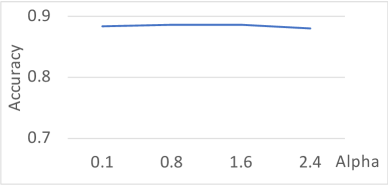
|
|
|
|||||||||||||||
| TP | FP | Acc | TP | FP | Acc | TP | FP | Acc | |||||||||
| 900 | 198 | 19 | 0.883 | 157 | 19 | 0.849 | 95 | 58 | 0.836 | ||||||||
| 1200 | 203 | 30 | 0.876 | 175 | 39 | 0.847 | 105 | 53 | 0.859 | ||||||||
| 1600 | 210 | 46 | 0.864 | 200 | 46 | 0.870 | 108 | 77 | 0.827 | ||||||||
|
|
|
|
||||||||||||||||
| TP | FP | Acc | TP | FP | Acc | TP | FP | Acc | |||||||||||
| 0.9 | 145 | 4 | 0.837 | 115 | 9 | 0.807 | 234 | 47 | 0.799 | ||||||||||
| 0.8 | 160 | 13 | 0.844 | 149 | 39 | 0.812 | 242 | 46 | 0.809 | ||||||||||
| 0.7 | 204 | 32 | 0.874 | 178 | 90 | 0.783 | 175 | 13 | 0.770 | ||||||||||
| TrojAI R2 | TrojAI R3 | TrojAI R4 | |||||||||||||||||||||||||||||||||
|
|
|
|
|
|
||||||||||||||||||||||||||||||
| TP | FP | Acc | TP | FP | Acc | TP | FP | Acc | TP | FP | Acc | TP | FP | Acc | TP | FP | Acc | ||||||||||||||||||
| Middle | 215 | 54 | 0.861 | 220 | 97 | 0.815 | 205 | 100 | 0.806 | 153 | 58 | 0.792 | 102 | 75 | 0.821 | 257 | 77 | 0.791 | |||||||||||||||||
| Second Last | 198 | 19 | 0.883 | 204 | 32 | 0.874 | 182 | 68 | 0.818 | 149 | 39 | 0.812 | 105 | 53 | 0.859 | 242 | 46 | 0.809 | |||||||||||||||||
| Last | 141 | 6 | 0.83 | 171 | 16 | 0.854 | 159 | 65 | 0.791 | 141 | 27 | 0.817 | 84 | 37 | 0.852 | 196 | 37 | 0.766 | |||||||||||||||||
Appendix C More Details of the Model Repair Experiment
We show the trigger size for each label pair for an trojaned model in Table 21 and for an benign model in Table 22. Table 21 (a) shows the trigger size between each pair of labels. The columns denote the victim label and the rows denote the the target label. For example, the gray cell in Table 21 (a) shows the trigger size to flip class 1 to class 0. Table 21 (b) follows the same format and shows the result for trojaned model after unlearning. In the trojaned model the injected trigger flips class 1 to class 0. Before unlearning, class 1 and class 0 have the smallest trigger size 21. Unlearning increases the trigger size between the two to 106, which is above the average trigger size between any pairs. Intuitively, one can consider the backdoor is fixed. In the benign model, the natural trigger flips class 3 to class 5. As shown in Table 22, unlearning only increases the trigger size from 24 to 59 and 59 is still one of the smallest trigger size among all label pairs for the fixed model.
| 0 | 1 | 2 | 3 | 4 | 5 | 6 | 7 | 8 | 9 | |
| 0 | - | 48 | 34 | 75 | 42 | 52 | 62 | 46 | 48 | 52 |
| 1 | 21 | - | 74 | 91 | 88 | 96 | 72 | 80 | 81 | 45 |
| 2 | 32 | 54 | - | 66 | 39 | 57 | 54 | 61 | 78 | 60 |
| 3 | 34 | 53 | 35 | - | 42 | 27 | 46 | 50 | 72 | 47 |
| 4 | 29 | 45 | 29 | 49 | - | 36 | 46 | 48 | 63 | 48 |
| 5 | 40 | 70 | 35 | 46 | 43 | - | 53 | 49 | 81 | 56 |
| 6 | 29 | 48 | 23 | 41 | 44 | 61 | - | 66 | 70 | 59 |
| 7 | 40 | 77 | 55 | 78 | 40 | 52 | 81 | - | 82 | 60 |
| 8 | 21 | 44 | 42 | 75 | 50 | 59 | 60 | 65 | - | 47 |
| 9 | 29 | 62 | 78 | 85 | 69 | 70 | 73 | 62 | 73 | - |
| 0 | 1 | 2 | 3 | 4 | 5 | 6 | 7 | 8 | 9 | |
| 0 | - | 84 | 56 | 103 | 77 | 96 | 82 | 96 | 56 | 78 |
| 1 | 106 | - | 132 | 162 | 150 | 140 | 113 | 134 | 124 | 70 |
| 2 | 92 | 111 | - | 88 | 79 | 79 | 62 | 99 | 109 | 106 |
| 3 | 105 | 92 | 66 | - | 86 | 60 | 58 | 82 | 124 | 86 |
| 4 | 96 | 92 | 55 | 81 | - | 72 | 53 | 77 | 99 | 95 |
| 5 | 119 | 100 | 64 | 70 | 91 | - | 58 | 101 | 136 | 90 |
| 6 | 107 | 97 | 86 | 88 | 99 | 93 | - | 113 | 113 | 97 |
| 7 | 94 | 101 | 92 | 124 | 87 | 87 | 81 | - | 126 | 100 |
| 8 | 50 | 72 | 68 | 104 | 98 | 106 | 81 | 101 | - | 79 |
| 9 | 104 | 87 | 129 | 119 | 117 | 115 | 110 | 108 | 123 | - |
| 0 | 1 | 2 | 3 | 4 | 5 | 6 | 7 | 8 | 9 | |
| 0 | - | 43 | 44 | 47 | 38 | 42 | 67 | 68 | 37 | 48 |
| 1 | 62 | - | 89 | 88 | 79 | 78 | 70 | 85 | 76 | 47 |
| 2 | 53 | 58 | - | 37 | 35 | 42 | 51 | 71 | 72 | 62 |
| 3 | 62 | 66 | 40 | - | 40 | 24 | 48 | 59 | 72 | 56 |
| 4 | 61 | 57 | 38 | 48 | - | 31 | 52 | 52 | 85 | 64 |
| 5 | 69 | 66 | 43 | 33 | 46 | - | 51 | 61 | 73 | 57 |
| 6 | 66 | 55 | 32 | 35 | 44 | 38 | - | 80 | 87 | 62 |
| 7 | 74 | 77 | 67 | 61 | 38 | 39 | 74 | - | 92 | 68 |
| 8 | 29 | 44 | 55 | 61 | 48 | 51 | 62 | 65 | - | 46 |
| 9 | 79 | 57 | 84 | 72 | 67 | 67 | 83 | 76 | 72 | - |
| 0 | 1 | 2 | 3 | 4 | 5 | 6 | 7 | 8 | 9 | |
| 0 | - | 79 | 56 | 89 | 63 | 90 | 65 | 99 | 59 | 76 |
| 1 | 120 | - | 134 | 114 | 123 | 154 | 77 | 119 | 122 | 48 |
| 2 | 95 | 101 | - | 75 | 58 | 74 | 59 | 82 | 121 | 82 |
| 3 | 104 | 98 | 57 | - | 58 | 59 | 40 | 90 | 124 | 80 |
| 4 | 104 | 100 | 60 | 88 | - | 79 | 50 | 73 | 117 | 79 |
| 5 | 95 | 91 | 58 | 84 | 76 | - | 52 | 77 | 131 | 86 |
| 6 | 114 | 115 | 77 | 129 | 102 | 89 | - | 131 | 137 | 93 |
| 7 | 104 | 120 | 110 | 103 | 68 | 92 | 66 | - | 129 | 78 |
| 8 | 36 | 61 | 74 | 80 | 66 | 112 | 66 | 86 | - | 70 |
| 9 | 128 | 109 | 117 | 103 | 112 | 120 | 73 | 124 | 105 | - |