Evidence for a rapid decrease of Pluto’s atmospheric pressure revealed by a stellar occultation in 2019

The occultation of a star UCAC5 340-173206 (Gaia DR2 catalog source ID: 6772059623498733952, ICRS position at epoch J2000: $\alpha=19^{\rm h}\leavevmode\nobreak\ 33^{\rm m}\leavevmode\nobreak\ 26^{\rm s}.013$, $\delta=-22\degr\leavevmode\nobreak\ 07^{\prime}\leavevmode\nobreak\ 58.42"$, Gaia Gmag = 13.0; Gaia Collaboration. 2018) on 2019 July 17 was originally predicted by ERC Lucky Star project¹¹1http://lesia.obspm.fr/lucky-star/occ.php?p=13163. The project predicts stellar occultations by Pluto using Numerical Integration of the Motion of an Asteroid (NIMA) version 8 orbital elements (Desmars et al., 2019). The prediction confirmed that Pluto’s shadow swept over the major islands of Hawaii at a geocentric velocity $v_{\rm rel}=24.18\leavevmode\nobreak\ {\rm km\leavevmode\nobreak\ s^{-1}}$. The geocentric distance of Pluto during the occultation corresponds to $D=32.83\leavevmode\nobreak\ {\rm au}$.

On 2019 July 17, we observed UCAC5 340-173206 at the Tohoku University Haleakala Observatory (latitude: $20\degr$ $42^{\prime}$ $30"$ N, longitude: $156\degr 15^{\prime}30"$ W, altitude: 3040 m), Hawaii. At Haleakala, photometric data were obtained using a ZWO Co., Ltd. ASI178MM CMOS camera mounted on the Coude focus of the Tohoku University 60 cm Cassegrain / Coude (T60) telescope. The field of view (FoV) for the CMOS camera is $120\arcsec\times 80\arcsec$ with an angular pixel scale of 0.″038. The exposure time was 2 s for each frame corresponding to the frame rate of $\sim 0.5\leavevmode\nobreak\ {\rm Hz}$. No filter was used in the present observation. During the observation, a dataset consisting of 1305 image frames were obtained in a 43.5-minute window centered on the predicted central time of the occultation (12:42 on 2019 July 17 UTC) with an imaging capture software Firecapture version 2.4.

Aperture photometry for the occulted star (plus Pluto and Charon) is performed using the image data after the bias and flat-field corrections and the sky background subtraction. Due to possible rapid changes in atmospheric conditions, the obtained flux values for individual data points can suffer time-dependent flux fluctuations. To correct the possible flux fluctuations and calibrate the flux value of the target star, we carry out differential photometry with three reference stars (Gaia DR2 G-band magnitude range of $11-14$) that are detected simultaneously. The calibrated light curve is then normalized to the unocculted flux.

We also obtained a Pluto $+$ Charon flux relative to the total flux (including the occulted star) with resolved images obtained approximately 40 minutes before the occultation event. To obtain an accurate Pluto $+$ Charon flux, we subtract a radial brightness profile of UCAC5 340-173206 located close to Pluto and Charon in the original images based on a digital coronagraphic method developed by Assafin et al. (2009). The derived relative flux ratio is $\sim 0.241$. We should note that, however, the imperfect flat-field correction, the residual of the stellar radial brightness profile, the airmass variation (1.5 during calibration versus 1.7 during the occultation), and Pluto’s rotational albedo variation can cause a systematic uncertainty of the flux ratio. We thus use this flux ratio only as a reference value for the light curve fit (see Section 3.1).

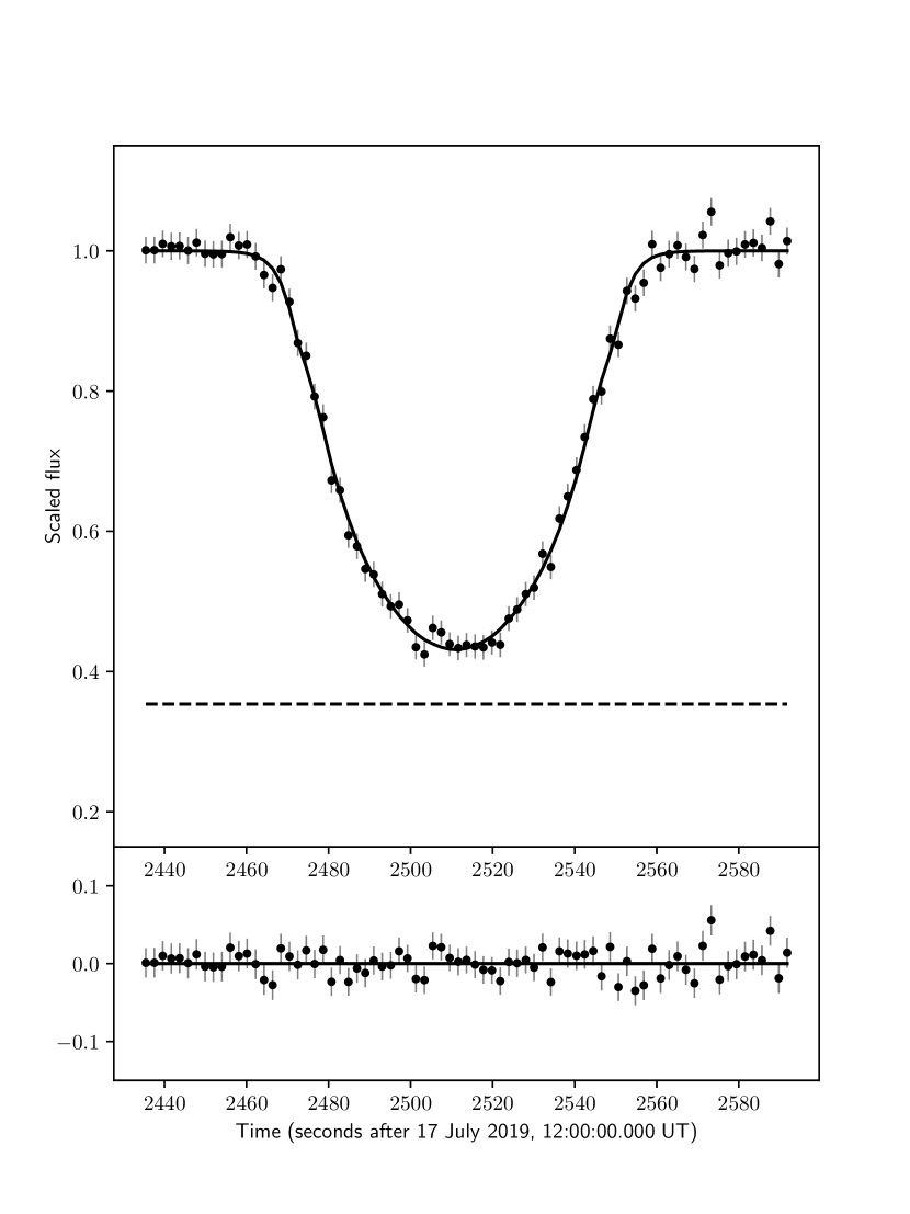
Figure 1 shows the light curve of the target star after the calibration and the normalization. The observed duration of the occultation is roughly $\sim 50$ s. No significant asymmetric profile or spike-like feature was detected from the light curve. To obtain the pressure of the atmosphere, synthetic light curves as a function of the pressure at a radius of $r=1215\leavevmode\nobreak\ {\rm km}$, which has been referred to be a reference radius by previous studies (Yelle, & Elliot, 1997; Sicardy et al., 2016; Meza et al., 2019), $p_{1215}$, the distance of closest approach of Haleakala Observatory to Pluto’s shadow center, $\rho$ the central time of the occultation, and the Pluto $+$ Charon flux relative to the total flux, are generated using a ray-tracing technique described by Sicardy et al. (1999). For Pluto’s atmospheric refraction model, we consider atmospheric profiles provided by Dias-Oliveira et al. (2015) with assumptions that Pluto has a pure ${\rm N_{2}}$, spherically symmetric and transparent (haze-free) atmosphere with a time-independent thermal structure derived from the observed light curves. In the present model, the contribution from the near-limb (primary) image and far-limb (secondary) images are considered with a focusing factor (the ratio of the observer’s distance to the shadow center and the closest approach of the corresponding ray in Pluto’s atmosphere assuming a circular limb curvature of Pluto) provided by Sicardy et al. (1999). The validity of these assumptions is discussed by Meza et al. (2019) with the NH results. According to Meza et al. (2019), the fixed temperature profile appears to be close to the results derived from NH and is thus useful for at least estimating the relative pressure changes. The physical parameters used for the fit are presented in Table 1. We adopted these parameters following Dias-Oliveira et al. (2015) and Meza et al. (2019) to avoid systematic uncertainties caused by using different values.

The synthetic light curve is fitted to the observed data points (77 data points shown in Figure 1 are used for the fit) by minimizing $\chi^{2}$;

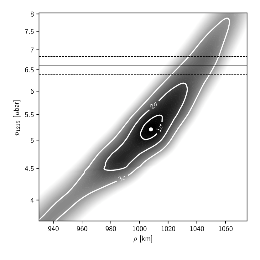
where $\phi_{i,{\rm obs}}$, $\phi_{i,{\rm syn}}$, and $\sigma_{i}$ are the observed and synthetic stellar fluxes, and the $1\sigma$ error at a data point $i$, respectively. Figure 2 shows the $\chi^{2}$ map for the fit to the light curve as a function of $p_{1215}$ and $\rho$. The $\chi^{2}$ value for the best fit is 61.9 with 73 degrees of freedom (corresponding to 77 data points - 4 free parameters), indicating a satisfactory fit with a reduced $\chi^{2}$ of $\sim 0.848$. The best-fit parameters are shown in Table 1, and the best-fit synthetic data points are overlaid with the observed data points in Figure 1. According to the best-fit model, observed stellar rays come from above $r\sim 1214\leavevmode\nobreak\ {\rm km}$, which is comparable to the adopted reference radius. The obtained reference radius pressure is $p_{1215}=5.20^{+0.28}_{-0.19}\leavevmode\nobreak\ {\rm\mu bar}$ ($1\sigma$ level error bars, see Figure 2). Assuming the lower atmosphere temperature profile provided by Dias-Oliveira et al. (2015), this value corresponds to a surface ($r=1187\leavevmode\nobreak\ {\rm km}$) pressure of $p_{\rm surf}=9.56^{+0.52}_{-0.34}\leavevmode\nobreak\ {\rm\mu bar}$.

The best-fit $\rho$ is derived to be $\rho=1008.0^{+7.8}_{-7.2}\leavevmode\nobreak\ {\rm km}$. The central time of the occultation derived from the fit is 12:41:$52.02\pm 0.18$ on 2019 July 17 UTC. We should note that the value derived from timestamps of the image data have a constant offset of several seconds due to imperfect time synchronizations of the capture software (Arimatsu et al., 2017). The best-fit Pluto $+$ Charon flux ratio is $0.261\pm 0.012$, which is slightly higher but comparable to that observed before the occultation event ($0.241$, see Section 2.2).

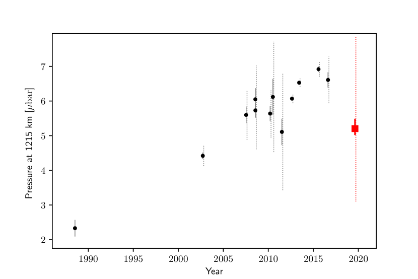
Figure 3 shows the reference radius pressure $p_{1215}$ as a function of time; our result is compared with pressure values obtained by previous studies (Meza et al., 2019) using the same atmosphere model profile. The present pressure value is the lowest among those reported after 2012. We report a diminution of pressure of $21^{+4}_{-5}\%$ ($1\sigma$ error bars) between 2016 (when $p_{1215}=6.61\pm 0.22\leavevmode\nobreak\ {\rm\mu bar}$, Meza et al. 2019) and our measurement in 2019 ($p_{1215}=5.20^{+0.28}_{-0.19}\leavevmode\nobreak\ {\rm\mu bar}$, see above). This corresponds to a decrease rate of $7.1^{+1.2}_{-1.7}\%$ per Earth year. Examination of the $\chi^{2}$ map in Figure 2, however, shows that this drop is detected at the $2.4\sigma$ level, and thus remains marginally significant. Previous occultation studies using the same atmospheric model profile have reported a continuous increase of the pressure by a factor of approximately three between 1988 and 2016 (Meza et al., 2019), corresponding to an average increase rate of $\sim 4\%$ per Earth year. Taken at face value, our result thus indicates that Pluto’s atmospheric pressure is decreasing nearly twice as rapidly as it increased in the previous three decades.