Evaluation of vacuum energy density around geometrical defects by the WKB method
Abstract
The energy density of a conformally invariant scalar field around a cosmic string is estimated by the WKB method. This approach reproduces the precise value obtained by the other authors using the exact mode-sum method or the method of mirror images. The approximation is also in good agreement with the exact result in the three-dimensional case. We also evaluate the energy density of a conformally invariant scalar field around a global monopole by the same way find the known result again.
pacs:
PACS number(s): 03.70.+k, 04.60.+n, 98.80.CqI Introduction
The vacuum energy of free fields on the conical space created by the presence of an idealized cosmic string V can be computed by the several ways qfcs . The metric describing an infinitely long straight cosmic string laid along the axis is given by V
| (1) |
where is a parameter that characterizes the cosmic string. Using this, the deficit angle is expressed as and the mass density of the string is . For a conformally invariant scalar field, the vacuum expectation value of the energy density at one-loop level in the spacetime described by the metric (1) has been found to be qfcs
| (2) |
In this paper, we evaluate the quantum vacuum energy of a conformally invariant scalar field using the WKB method. The derivation is simple and pedagogical: Moreover, this yields considerably accurate values in many cases. As a quantum field, we consider only a conformally invariant scalar field in this paper.
The organization of this paper is as follows. In Sec. II we study the WKB estimation of vacuum energy density of a conformally invariant scalar field around a straight cosmic string. The result is compared with the known one obtained by other methods. The technique is generalized to the cases of general spacetime dimensions in Sec. III. In Sec. IV, we treat vacuum energy around a global monopole. Sec, V is devoted to summary of the results.
II WKB evaluation of vacuum energy around a cosmic string
The vacuum energy at one-loop level arises from the zero-point energy of quantum fields cas . Formally, it is written by
| (3) |
where is the frequency of each normal mode in the expansion of the field. The subscript characterizes each normal mode. The formal expression (3) diverges due to unlimitedly high frequency modes. Therefore, to get a meaningful conclusion for the vacuum energy , we must regularize and subtract proper energy of standard, which is usually defined for a flat Minkowsky space.
We start with the expression (3) to obtain vacuum energy density in the spacetime described by the metric (1) representing the presence of a cosmic string. We demonstrate evaluation of the vacuum energy that comes from a conformally invariant scalar field governed by the Lagrangian
| (4) |
where is the scalar curvature and in the four-dimensional spacetime.
If the expression (3) is calculated naively, it is found to be divergent not only because of the unlimitedly high frequency modes but also because of the singularity of the space for the present case. On the dimensional ground, the energy density should be proportional to . Other length or mass scales are absent in the conformally invariant theory, at least in one-loop calculations. Thus our aim can be said to be determination of the coefficient of in the expression of the vacuum energy density.
The equation of motion for the scalar field is derived from (4) as
| (5) |
Now we define the following mode function:
| (6) |
where . Substituting the metric (1) and the mode function (6) into the wave equation (5), we get a differential equation for the radial function ,
| (7) |
To simplify the equation, we use the new coordinate defined by
| (8) |
where is an arbitrary constant. Then the differential equation concerning the radial function becomes
| (9) |
where
| (10) |
The solution according to the WKB approximation is given by
| (11) |
Suppose that the “wall” is located at , which is an infrared cutoff in some sense. On the other hand, near the conical singularity, we set a small cutoff at . We assume the boundary conditions at and . In this situation, a quantum number is associated with the radial wave function as
| (12) | |||||
Therefore the total number of wave modes per unit length along the cosmic string with the frequency is written by
| (13) |
where the sum over and integration over is taken just for real positive values of the integrand.
We now get the vacuum energy per unit length along the cosmic string,
| (14) | |||||
Changing the order of integration, we have
| (15) |
with
| (16) |
The integration over in (15) diverges in the limit , since “vacuum energy density” should be proportional to . Accordingly, we have only to manage the ultraviolet divergence in the formal expression of .
We again change the order of integration and perform the integration over first. We treat the divergent integration by analytical continuation. That is, the square root in the expression of is regarded as the th power. The outcome of the integration is
| (17) |
where the constant has the dimension of mass.
Next, we perform the integration over . Then we get
| (18) |
Discarding the term for , we can rewrite the above as
| (19) |
where is the Riemann’s zeta function.
Taking the limit in the context of analytic continuation, we find the following finite quantity:
| (20) | |||||
where the numerical values are substituted (see, for example, AS .).
Finally, the finite vacuum energy density is obtained by subtraction as
| (21) | |||||
This result coincides with the known result obtained by exact mode summation or mirror-image method qfcs .
We can also consider a “twisted” scalar field twist , which has a special periodicity in : . For the twiwted field, the vacuum energy can be obtained by replacing . Thus the vacuum energy density before subtraction is derived as
| (22) |
Then the finite vacuum energy density is given by
| (23) | |||||
which also turns out to be the exact expression qfcs .
In the next section, the procedure of evaluation of vacuum energy is generalized to an arbitrary dimensional case.
III Vacuum energy for a conical defect in general dimensions
In this section, we consider a conical singularity in general dimensions. The -dimensional metric is written by
| (24) |
The Lagrangian for a conformal scalar field is the same as (4), except for .
The evaluation of vacuum energy density of a conformal scalar field in this spacetime is done by a similar way that we showed in the preceding section. In our methods, the unregularized energy density per unit -volume can be expressed as
| (25) |
The difference from the previous section is the dimension of the integration over ’s. Carrying out the integration over and arranging the sum over , we have
| (26) |
Further applying the reciprocal formula for zeta and gamma functions Er
| (27) |
to (26), we obtain
| (28) |
where the limit has been taken.
Consequently, the regularized vacuum energy density for an untwisted conformal scalar filed is given by
| (29) | |||||
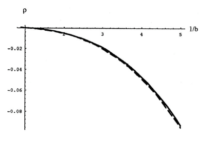
An exact result for has been shown by Souradeep and Sahni SS . Their result is given by the form of integration,
| (30) |
where the notation has been changed into ours.
The comparison between the exact and approximate results is displayed in FIG. 1. We conclude that the result of the WKB approximation is in excellent agreement with the exact value for the three-dimensional case ().
IV Vacuum energy around a global monopole
A global monopole BV can be regarded as a geometrical point singularity with a deficit solid angle, if the finite-mass contribution is neglected. The metric of the spacetime describing a global monopole is
| (32) |
It is possible to generalize the metric to the ()-dimensional one,
| (33) |
where is a line element on an -sphere with a unit radius.
The derivation of the formal expression for the vacuum energy of a conformal scalar field in the spacetime described by the metric (33) can be done similarly to that in the previous sections.
We have only to notice a few differences.
-
•
The coupling to the scalar curvature is now .
-
•
The value of the scalar curvature is nonzero for .
-
•
The mode function takes the form
where is the generalized spherical function whose eigen value for the laplacian on is .
Hence we obtain
| (34) |
where
| (35) |
and
| (36) |
The choice and leads to the vacuum energy around a cosmic string (18), etc..
Various ways to regularize the divergent quantity are known CW . Instead of investigating general treatment, we study here the “original” case with the metric (32) ( and ), i.e., the case with a global monopole at the origin. The generalization of this example to other cases is straightforward.
For the first three terms in the sum diverges as in the limit , we introduce the renormalization scale , which involves the mass parameter . We can regard that the divergence and other finite terms are absorbed into the choice of the renormalization scale.
Then we get the following expression in the limit of :
| (41) |
The result should be compared with the one obtained by Mazzitelli and Lousto ML . In our notation, their result in ML should read as
| (42) |
since a factor two has been missed there (cf. BD ).
One can easily find that this coincides with the vacuum energy density obtained by our WKB approach , where is given in (41).
V Summary
We have shown the validity of the WKB method to obtain one-loop vacuum energy density of a conformally invariant scalar field around geometrical defects.
In particular, for the case with a straight casmic string in four dimensional spacetime, we have found that the WKB evaluation reproduces an exact value of the vacuum energy density for untwisted or twisted conformal scalar fields. In the case with a three-dimensional conical spacetime, the WKB result is not an exact value but an excellent approximation of the vacuum energy density for a conformally invariant scalar field. The vacuum energy density around a global monopole has been calculated by the WKB method for a conformally invariant scalar field. The result coincides with the one obtained by another method.
The varidity of our WKB approach is ensured by the following.
-
•
The background metric of the present model contains no dimensionful constants except for .
-
•
The Lagrangian for a scalar field in the present model is conformally invariant.
-
•
The regularized quantity is considered to be largely relied on the divergence from rather high frequency modes.
It will be worth studying generalization of the WKB method to evaluation of free energy density of quantum fields in finite-temperature system with geometrical defects.
References
- (1) A.Vilenkin, Phys. Rev. D23, 852 (1981); Phys. Rep. 121, 263 (1985).
-
(2)
B. Linet, Phys. Rev. D35, 536 (1987).
J. S. Dowker, Phys. Rev. D36, 3742 (1987).
A. Sarmient and S. Hacyan, Phys. Rev. D38, 1331 (1988).
A. G. Smith, in The Formation and Evolution of Cosmic Strings, edited by G. Gibbons, S. Hawking and T. Vachaspati (Cambridge University Press, Cambridge, 1989), P. 263.
K. Shiraishi and S. Hirenzaki, Class. Q. Grav. 9, 2277 (1992).
M. E. X. Guimarães and B. Linet, Commun. Math. Phys. 165 297, (1994). -
(3)
G. Plunien, B. Müller and W. Greiner,
Phys. Rep. 134, 87 (1986).
E. Elizarde et al., Zeta Regularization Techniques with Applications (World Scientific, Singapore, 1994). - (4) M. Abramowitz and I. A. Stegun (eds.), Handbook of mathematical functions (Dover, New York, 1972).
-
(5)
C. J. Isham, Proc. R. Soc. London
A362, 383 (1978); A364, 591 (1978).
L. H. Ford, Phys. Rev. D21, 949 (1980). - (6) A. Erdélyi et al. (eds.) Higher transcendental functions (McGraw-Hill, New York, 1955).
- (7) T. Souradeep and V. Sahni, Phys. Rev. D46, 1616 (1992).
- (8) M. Barriola and A. Vilenkin, Phys. Rev. Lett. 63, 341 (1989).
- (9) P. Candelas and S. Weinberg, Nucl. Phys. B237, 397 (1984).
- (10) F. D. Mazzitelli and C. O. Lousto, Phys. Rev. D43, 468 (1991).
-
(11)
N. D. Birrell and P. C. W. Davies,
Quantnm fields in curved space
(Cambridge University Press, Cambridge, 1982), chapter 6.
S. M. Christensen, Phys, Rev. D17, 946 (1978).