Evaluating Treatment Benefit Predictors using Observational Data: Contending with Identification and Confounding Bias
Abstract
A treatment benefit predictor (TBP) maps patient characteristics into an estimate of the treatment benefit for that patient, which can support optimizing treatment decisions. However, evaluating the predictive performance of a TBP is challenging, as this often must be conducted in a sample where treatment assignment is not random. After briefly reviewing the metrics for evaluating TBPs, we show conceptually how to evaluate a pre-specified TBP using observational data from the target population for a binary treatment decision at a single time point. We exemplify with a particular measure of discrimination (the concentration of benefit index) and a particular measure of calibration (the moderate calibration curve). The population-level definitions of these metrics involve the latent (counterfactual) treatment benefit variable, but we show identification by re-expressing the respective estimands in terms of the distribution of observable data only. We also show that in the absence of full confounding control, bias propagates in a more complex manner than when targeting more commonly encountered estimands (such as the average treatment effect). Our findings reveal the patterns of biases are often unpredictable and general intuition about the direction of bias in causal effect estimates does not hold in the present context.
Keywords: calibration; discrimination; confounding bias; precision medicine.
Introduction
Precision medicine aims to optimize medical care by tailoring treatment decisions to the unique characteristics of each patient. This objective naturally falls in the intersection between predictive analytics and causal inference; the former aims at predicting the outcome of interest given salient patient characteristics, and the latter seeks to answer counterfactual “what if” questions about the outcome. Most progress in clinical prediction models has centered around estimating the risk of adverse outcomes, often guiding treatment decisions by prioritizing high-risk individuals for intervention [1, 2]. However, the success of such guidance relies on an implicit assumption: that those classified as high risk are also those who will benefit the most from the treatment. A more relevant approach for decision-making is to directly predict treatment benefits based on patient characteristics. In this context, treatment benefit refers to the conditional risk reduction for treated individuals given their characteristics, compared to the conditional risk they would face under identical conditions without the treatment. This comparison, which is hypothetical, requires causal reasoning to predict [3]. Such a prediction is often termed “causal prediction” or “counterfactual prediction” [4]. In causal inference, the treatment benefit we are predicting is the conditional average treatment effect (CATE).
We are interested in a function that maps a patient’s characteristics to their putative treatment benefit, which we call a treatment benefit predictor (TBP). Suppose we have a pre-specified TBP developed from a randomized controlled trial (RCT) in one setting, where it demonstrates strong predictive performance. Before being adopted into patient care for the target population with a potentially distinct setting, this TBP needs to be evaluated (validated) [5, 6]. Transportability and generalizability have been studied across various epidemiology-adjacent disciplines, focusing on concepts, assessment methods, and correction techniques, most of which require access to both original and target population data. This includes applications in estimating causal estimands (e.g. average treatment effect (ATE)) [7], identifying causal relations [8], and predicting outcome risks [9] in the target population. However, we do not aim to assess or correct the transportability and generalizability of the pre-specified TBP, as we only have access to data from the target population. Instead, we focus on the predictive performance metrics, though transportability and generalizability may naturally be implied by these results, e.g. if we find the TBP performs well.
Traditionally, performance metrics for risk prediction are categorized into measures of overall fit (e.g. Brier score), discrimination (e.g. c-statistic), and calibration (e.g. calibration plot) [10, 11]. Various performance measures for TBPs have been formulated by extending the concepts from risk prediction to the treatment-benefit paradigm. The overall fit of a TBP is typically evaluated by the discrepancy between predicted treatment benefits and estimated CATE, using metrics like the precision in estimating heterogeneous effects [12, 13]. The discriminative ability reflects the degree to which TBP ranks patients in the correct order of treatment benefit. For instance, the c-for-benefit proposed by van Klaveren et al. is an extension of the c-statistic [14]. However, some possible limitations of the c-for-benefit have been discussed [9, 15, 16]. In particular, it has been shown to lack the properties of a proper scoring rule [17]. Other metrics of discriminatory performance are the concentration of the benefit index () [18] and the rank-weighted average treatment effect metrics [19], which are extended from the relative concentration curve (RCC) [20] and Qini curve [21], respectively. Both metrics compare how individuals prioritized by TBP predictions benefit more from treatment than those selected randomly. Note that RCCs and Qini curves are conceptually related to the Lorenz curve and the Gini index [22]. Calibration evaluates the agreement between the predicted and the actual quantities. Van Calster et al. proposed a hierarchical definition in the context of risk prediction [23]. Researchers have extended the ‘weak calibration’ to assess the performance of TBPs via the calibration intercept and slope [9, 16]. They have also extended the ‘moderate calibration’ to examine whether the conditional expected treatment benefit given TBP prediction, equals the TBP prediction [24].
None of these extensions are straightforward, given the unavailability of the counterfactual outcome. Another challenge arises when evaluating TBP performance using observational studies, as these introduce potential confounding bias. This is especially relevant when RCTs are unavailable, underpowered, or not representative of the target population. Additionally, for some interventions where equipoise is not established, conducting a RCT might be unethical.
In this study, we show conceptually how to approach evaluating a TBP from observational data, focusing on a single time-point binary treatment decision. Specifically, for several measures of TBP performance, we re-express the metrics, initially defined in terms of the latent treatment benefit variable, in terms of the distribution of observable quantities. To illustrate, we focus on two existing performance metrics for assessing pre-specified TBPs: and the moderate calibration curve. Additionally, we pay close attention to the bias incurred if we are not fully controlling for confounding. In doing so, we extend the understanding of identification and confounding bias from the context of well-understood estimands such as ATE to estimands which describe the predictive performance of a pre-specified TBP [25, 26]. Some applied problems have more complex settings than those of a single time-point binary treatment choice. For instance, a recent study extended the definitions and estimators of calibration and discrimination metrics to time-to-event outcomes and time-varying treatment decisions[27]. However, their focus was not on evaluating predictive performance in scenarios where confounding is not fully controlled or on exploring confounding bias in this context.
Notation and Assumptions
Each individual in the target population is described by with joint distribution . Here denotes a binary treatment, and is the counterfactual outcome that would be observed under treatment , where . A larger is presumed to be the preferred outcome. The set consists of pre-treatment covariates that are observable in routine clinical practice and in observational studies, and are used to predict treatment benefit. In contrast, is a distinct set of covariates that may only be available in the observational study and could be necessary for controlling confounding. Both and may include a mix of continuous and discrete variables. For instance, could be blood pressure and obesity, available at the point of care, which are used to predict the benefit of statin therapy for cardiovascular diseases. Meanwhile, could be socioeconomic status, which is a confounding variable but not often used for predicting benefit from statins.
Individual treatment benefit is quantified as , which is unobservable. For instance, when an individual has received , the corresponding outcome remains unobserved (and therefore counterfactual). We denote the mean treatment benefit for groups partitioned by both and as . However, in clinical practice, the ideal quantity to inform treatment decisions for an individual with is , which conditions only on . Denote the common causal estimand ATE as . A TBP predicting the mean treatment benefit based on patient characteristics is denoted as . This can guide treatment decision-making, for example the care provider offering treatment only to those with . We denote the predicted treatment benefit from as . The best possible TBP is itself, and the corresponding prediction is .

Observed data from the observational study are realizations of a set of random variables drawn from an underlying probability distribution , denoted as , which is a consequence of . We define and . We denote the propensity score as .
To ensure that can be identified from the observed data, must have a causal interpretation. Therefore, the following assumptions are universally required: (1) no interference: between any two individuals, the treatment taken by one does not affect the counterfactual outcomes of the other; (2) consistency: the counterfactual outcome under the observed treatment assignment equals the observed outcome ; and (3) conditional exchangeability: the treatment assignment is independent of the counterfactual outcomes, given the set of variables ; (4) overlap (positivity): the conditional probability of receiving the active treatment or not is bounded away from and , i.e., , for all possible and . The first two assumptions are known as the stable-unit-treatment-value assumption (SUTVA) [28]. The third one assumes no unmeasured confounders given and , as illustrated in Figure S1.
Predictive Performance Metrics
Given a pre-specified TBP , we intend to evaluate its predictive performance on observational data from the target population. Among all possible predictive performance metrics for evaluating TBP, we exemplify with two metrics by specifying the estimand of each, which helps conceptually in understanding how to measure the predictive performance of using observational data.
Discrimination
The concentration of the benefit index () is a single-value summary of the difference in average treatment benefit between two treatment assignment rules: ‘treat at random’ and ‘treat greater .’ [18] With i.i.d. copies of , the of is defined as:
| (1) |
where is an indicator function. The numerator in Equation (1) operationalizes the strategy of ‘treat at random’ among two patients randomly selected from the population, and the denominator refers to the strategy of ‘treat greater .’ If the two patients have the same , treatment is randomly assigned to one of them. When and is at least not worse than ‘treat at random,’ . A value of can be interpreted as indicating that ‘treat at random’ is associated with a reduction in expected benefit compared with ‘treat greater .’ Therefore, the higher the value of , the stronger the discriminatory ability of .
We note that can be calculated by approaching the cumulative distribution function (CDF) and the probability mass function (PMF) of , thereby eliminating the necessity of considering patient pairs to ascertain the expectation in Equation (1). Therefore, we reexpress the of as
where , denotes CDF of , and is PMF of . This expression clearly indicates that summarizes the predictive performance of based on its ranking ability. The calculation process is simplified by focusing on , , and , and it becomes even simpler when is continuous, as . Although is continuous in most applications, it is helpful to derive the general expression to create illustrative examples where is discrete. As the original publication on did not discuss estimation in the presence of ties, we elaborate on this point and give a derivation of why we are able to consider CDF of (and its PMF if necessary) in Appendix S1.
Calibration
The concept of moderate calibration for risk prediction is that the expected value of the outcome among individuals with the same predicted risk is equal to the predicted risk [23]. Similarly, in treatment benefit prediction, a can be considered moderately calibrated if for any ,
where is the moderate calibration function. The equality above states that the average treatment benefit among all patients with predicted treatment benefit equals . For example, if is moderately calibrated and predicts a group of individuals to have , we should expect that the average treatment benefit within the group is also . Furthermore, is strongly calibrated if . Calibration of TBPs can also be visualized in a calibration plot [29]. The calibration plot compares against , with a moderately calibrated TBP showing points on the diagonal identity line.
Estimands for metrics
These predictive performance metrics for TBP involve the latent variable . To evaluate a pre-specified using observational data, we need to specify estimands for each metric so that they can be identified using observable data. We adjust for confounding by expressing the estimands in terms of , even though TBP is solely a function of . To compute of , we re-express as
Similarly, to evaluate the moderate calibration of any , we need to determine (i.e., the moderate calibration curve), which can be obtained by taking the average of conditional on :
Note that , which plays a vital role in the determination of both and , is identifiable through the expression: . Alternately, it can be expressed as . These two expressions are equivalent at the population-level. However, variations may emerge when considering specific finite-sample estimating techniques associated with each expression. We will return to the finite-sample estimation of the and calibration curve in the discussion section.
Confounding Bias of Performance Metrics
If we treat the observational data as if they arose from a RCT, or if we do not sufficiently control for confounding, confounding bias may emerge. It is essential to investigate this bias and grasp how the lack of full control for confounding might affect the accuracy of our TBP performance evaluations. We focus on the confounding bias that occurs when alone is insufficient to control for confounding and denote the bias as a function of , which is
where is obtained by taking the expectation of over . To illustrate the propagation of to performance measures, we denote the inaccurate and , calculated without controlling for , as and , respectively.
The bias of and the bias function of the moderate calibration curve, , will be influenced by . For , this bias affects the identification of both and . The discrepancy from actual is , while the deviation from is . However, expressing the bias of is complex as it involves the difference between two ratios, which is in the form of:
| (2) |
This bias value depends on , and .
For , the deviation from the accurate assessment can be expressed as
| (3) |
which is a function of . It depends on and the association between and .
According to Equation (2) and Equation (3), the deviations in and moderate calibration may yield zero value(s) even with non-zero . In particular, zero deviation in would occur when the numerator in Equation (2) equals zero, and zero deviations in moderate calibration curve would occur when for some . In the next section, we further investigate these biases in several illustrative examples to demonstrate how influences and propagates to the evaluation measures.
Evaluating TBP in Synthetic Populations
Synthetic Target Populations
To illustrate the evaluation of pre-specified TBPs and to explore the impact of confounding bias, we consider three synthetic target populations, described by the DAG in Figure S1. The synthetic populations were constructed based on the motivating example of evaluating pre-specified TBPs that predict the benefit of bronchodilator therapy for lung function measured by Forced Expiratory Volume in one second () using observational data from the target population. Meanwhile, the TBPs considered are functions of obesity and symptom severity, as variables which are often available in routine primary care and can be used to make treatment decisions. However, socioeconomic status, which is not usually available in RCT, needs to be adjusted for when evaluating the predictive performance of the TBP using observational data.
In synthetic population 1, obesity and symptom severity are binary variables, denoted as , and socioeconomic status is also binary denoted as . These covariates are dependent with the joint distribution . The exposure is a binary indicator for bronchodilator therapy, and the outcome, improvement, is measured by a binary indicator (), leading to . The probability of receiving bronchodilator therapy is . The probability of having improvement is affected by covariates and the exposure linearly: and . Then, .
In synthetic population 2, obesity, symptom severity, and socioeconomic status are independent continuous variables, each following a uniform distribution on the interval . The exposure is binary, and the probability of receiving bronchodilator therapy is directly influenced by the values of socioeconomic status, with . Outcome is a continuous variable, which has non-linear relationships with the exposure and covariates. These are given by and , where and base response function . A similar setup has been used by Foster and Syrgkanis [30]. From these population specifications, we can derive that , which shows that socioeconomic status contributes to explaining both the outcome and therapy assignment but is independent of treatment benefit conditional on .
The synthetic population 3 differs slightly from population 1 in that with , and inverse logit, rather than linear, functions are used: , , and . Both population 1 and 3 quantify the strength of confounding through parameters, but we use population 3 to explore the extent to which the strength of confounding affects the bias of and .
All proposed populations are sufficiently simple to provide closed-form descriptions of the predictive performance of TBPs using and , as well as how confounding bias propagates to the bias of and for some pre-specified TBPs. Next, we compare evaluation results for TBPs with and without controlling for using populations 1 and 2, and illustrate how and the bias of metrics are influenced by the strength of confounding in population 3.
Evaluating Results
We formulate four pre-specified TBPs to be evaluated in the synthetic population 1, which can be expressed in the form of
where are coefficients. In particular, is the mean of covariates with , and is designed to be moderately calibrated by carefully choosing the coefficients. Let , which is strongly calibrated, and . (See Appendix S2 for the detailed definitions of the coefficients for TBPs.)
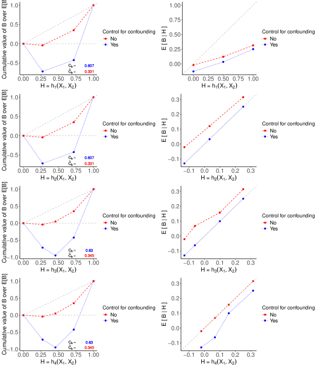
The evaluation results are illustrated in Figure S2, where the four plots on the left show the RCCs and values for the four TBPs, with and without bias. Note that and have identical discriminatory ability, as do and . This is because the CDFs of and are the same, as are those of and , resulting in the corresponding TBPs identically ranking patients. Note that and yield a slightly larger , compared to and . Consequently, and result in more effective treatment assignment rules, leading to larger average treatment benefits. Although values of suggest that and are more effective treatment assignment rules, they underestimate for all TBPs.
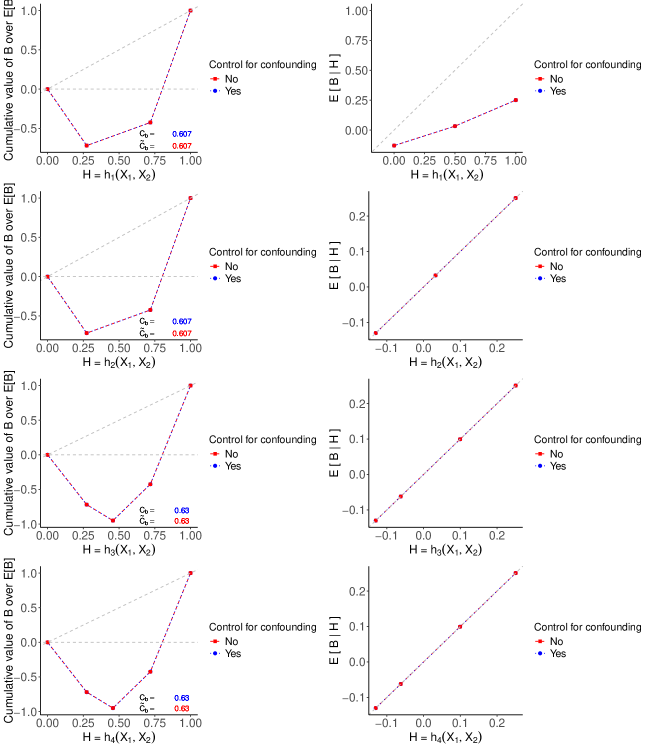
The four plots on the right in Figure S2 display the moderate calibration curves of all TBPs with and without bias. We see that and are moderately calibrated, aligning closely with the 45-degree line. Figure S2 highlights that the bias of the moderation calibration curve is positive for all values of all four TBPs due to . Consequently, the failure to fully control for confounding variables results in an inaccurate calibration assessment. The moderate calibration curve of suggests that a TBP developed in the target population, but without controlling for confounder , then it can give the misleading impression that it is moderately calibrated. When , all blue dotted curves align with the red dashed curves for both performance metrics because is no longer a confounding variable. (See Appendix S2 for the corresponding RCCs, , and calibration plots.) These findings highlight the importance of fully controlling for confounding variables, and ignoring confounding variables can produce misleading patterns.
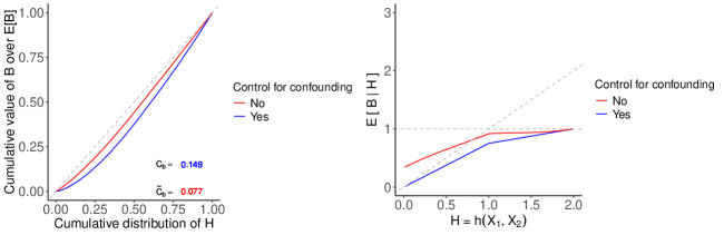
For synthetic population 2, we have , where follows a triangular distribution with parameters: lower limit , upper limit and mode . Using the knowledge of the population, we compute and then compare the two performance metrics with and without bias for in closed-form. (See Appendix S3 for calculation details.) In this setup, indicates that assigning treatment to a patient who has a larger value is slightly better than random treatment assignment. For the calibration curve, the average treatment benefit conditioned on the is when and is when .
However, confounding bias causes a deviation from the actual and the moderate calibration curve, which are depicted by Figure S3. The bias reduces the area between the independence line and the RCC by roughly half. It causes an overestimation of and an overestimation of . Consequently, , which is lower than the . Furthermore, in the calibration plot, the red curve deviates from the blue curve as the value of approaches zero. However, this deviation diminishes to zero as approaches two.
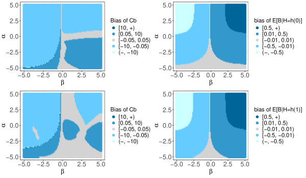
In synthetic population 3, the strength of confounding can be adjusted by the values of and . In Figure S4, the two plots on the right shows the relationship between and varying strengths of confounding, where and vary within the interval . For simplification, we focus on the special case where , and use the fact that the bias of the moderate calibration curve for equals when is a one-to-one mapping. Therefore, these two plots also displays the bias of the moderate calibration curve when and . The two plots on the left show the bias of under two different settings, highlighting the unpredictable pattern of bias and the strength of confounding. However, the pattern of bias in the moderate calibration curve is more interpretable compared to that of .
Discussion
In clinical settings, TBPs may offer valuable guidance for physicians and patients in making informed treatment decisions. Before being transported to a new population, these TBPs need to be evaluated in that population. Observational data, where treatment assignment is not random, might be the only opportunity for such evaluation. Consequently, addressing confounding bias is crucial when assessing TBPs based on observational data from the target population.
This study demonstrated conceptually how to evaluate pre-specified TBPs using observational data. We delved into two specific measures, and moderate calibration curve, which are estimands defined in terms of the latent benefit variable . We showed the identification of and by re-expressing the respective estimands in terms of the distribution of . The absence of full confounding control leads to bias in identifying and . The behavior of these biases are more complex than when targeting commonly encountered estimands such as ATE. We showed how the bias associated with , denoted as , propagates to that associated with and . We demonstrated the behaviors of these biases in two synthetic populations with . Positive function will always result in ; nevertheless, it might result for some choices of . In the two synthetic populations, we showed that positive functions lead to overestimation of and but underestimation of for our choices of . However, it is also possible that the overestimation of is greater than that of , leading to an overestimation of . When function takes both positive and negative values, behaviors of bias in identifying and become more unpredictable, making it difficult to intuit the specific direction of bias.
While we focused on population-level performance of TBPs and used synthetic populations, several findings from this study are relevant for practice. The primary objective of evaluating a pre-determined TBP is to estimate , for all possible and , from sample data. Estimating is a classical topic in the casual inference literature. For instance, it can be estimated through outcome regression, inverse probability weighting [31], or a combination of both, such as with the doubly robust method [32]. Additionally, Bayesian additive regression trees (BART) have been shown to offer several advantages in estimating CATE [12]. Building on the work presented here, we have initiated a new project that explores BART in TBP assessment using a real-world observational study.
Even with a scheme to estimate , further effect will be needed to estimate specific performance metrics, such as and the calibration curve. For instance, one possible estimator of uses sample averages to estimate expectations in the estimand and estimate the CDF of , and possibly its , through the empirical distribution of . For the calibration curve, the sample average within groups sharing the same can be used to estimate the conditional expectation of the estimated given when is discrete. For continuous , one approach is to discretize into equally sized bins and use the sample average within each bin to estimate the conditional expectation[24]. Moderate calibration can also be assessed non-parametrically, without the need for grouping or smoothing factors [33]. To our knowledge, this approach, based on the cumulative sum of prediction errors has yet to be applied to TBP assessment. Overall, exploring and tackling the challenges associated with estimating different performance measures is worthwhile.
In summary, we presented a conceptual framework for evaluating the predictive performance of TBPs using observational data. We demonstrated that in the absence of complete confounding control, the unpredictable nature of bias can significantly impact the reliability of TBP assessments. Moreover, this framework can be readily applied to practical settings, enabling the estimation of performance metrics such as and calibration curves.
References
- 1. Sperrin M, Martin GP, Pate A, Van Staa T, Peek N, Buchan I. Using marginal structural models to adjust for treatment drop-in when developing clinical prediction models. Statistics in medicine. 2018;37(28):4142–4154.
- 2. Sperrin M, Diaz-Ordaz K, Pajouheshnia R. Invited commentary: treatment drop-in—making the case for causal prediction. American journal of epidemiology. 2021;190(10):2015–2018.
- 3. Geloven N, Swanson SA, Ramspek CL, et al. Prediction meets causal inference: the role of treatment in clinical prediction models. European journal of epidemiology. 2020;35:619–630.
- 4. Prosperi M, Guo Y, Sperrin M, et al. Causal inference and counterfactual prediction in machine learning for actionable healthcare. Nature Machine Intelligence. 2020;2(7):369–375.
- 5. Roi-Teeuw HM, Royen FS, Hond A, et al. Don’t be misled: Three misconceptions about external validation of clinical prediction models. Journal of Clinical Epidemiology. 2024:111387.
- 6. Riley RD, Archer L, Snell KI, et al. Evaluation of clinical prediction models (part 2): how to undertake an external validation study. BMJ. 2024;384.
- 7. Degtiar I, Rose S. A review of generalizability and transportability. Annual Review of Statistics and Its Application. 2023;10(1):501–524.
- 8. Pearl J, Bareinboim E. Transportability of causal and statistical relations: A formal approach. in Proceedings of the AAAI Conference on Artificial Intelligence;25:247–254 2011.
- 9. Efthimiou O, Hoogland J, Debray TP, et al. Measuring the performance of prediction models to personalize treatment choice. Statistics in medicine. 2023;42(8):1188–1206.
- 10. Riley RD, Snell KI, Moons KG, Debray TP. Fundamental statistical methods for prognosis research. in Prognosis Research in Health Carech. 3, :37–68Oxford University Press 2019.
- 11. Steyerberg EW. Clinical Prediction Models. Springer International Publishing 2019.
- 12. Hill JL. Bayesian nonparametric modeling for causal inference. Journal of Computational and Graphical Statistics. 2011;20(1):217–240.
- 13. Schuler A, Baiocchi M, Tibshirani R, Shah N. A comparison of methods for model selection when estimating individual treatment effects. arXiv preprint arXiv:1804.05146. 2018.
- 14. Klaveren D, Steyerberg EW, Serruys PW, Kent DM. The proposed ‘concordance-statistic for benefit’ provided a useful metric when modeling heterogeneous treatment effects. Journal of Clinical Epidemiology. 2018;94:59–68.
- 15. Klaveren D, Maas CC, Kent DM. Measuring the performance of prediction models to personalize treatment choice: Defining observed and predicted pairwise treatment effects. Statistics in Medicine. 2023;42(24):4514–4515.
- 16. Hoogland J, Efthimiou O, Nguyen TL, Debray TP. Evaluating individualized treatment effect predictions: A model-based perspective on discrimination and calibration assessment. Statistics in medicine. 2024.
- 17. Xia Y, Gustafson P, Sadatsafavi M. Methodological concerns about “concordance-statistic for benefit” as a measure of discrimination in predicting treatment benefit. Diagnostic and Prognostic Research. 2023;7(1):10.
- 18. Sadatsafavi M, Mansournia MA, Gustafson P. A threshold-free summary index for quantifying the capacity of covariates to yield efficient treatment rules. Statistics in Medicine. 2020;39:1362–1373.
- 19. Yadlowsky S, Fleming S, Shah N, Brunskill E, Wager S. Evaluating treatment prioritization rules via rank-weighted average treatment effects. Journal of the American Statistical Association. 2024(just-accepted):1–25.
- 20. Yitzhaki S, Olkin I. Concentration indices and concentration curves. Lecture Notes-Monograph Series. 1991:380–392.
- 21. Radcliffe N. Using control groups to target on predicted lift: Building and assessing uplift model. 2007.
- 22. Gastwirth JL. The estimation of the Lorenz curve and Gini index. The review of economics and statistics. 1972:306–316.
- 23. Van Calster B, Nieboer D, Vergouwe Y, De Cock B, Pencina MJ, Steyerberg EW. A calibration hierarchy for risk models was defined: from utopia to empirical data. Journal of Clinical Epidemiology. 2016;74:167–176.
- 24. Xu Y, Yadlowsky S. Calibration error for heterogeneous treatment effects. in International Conference on Artificial Intelligence and Statistics:9280–9303PMLR 2022.
- 25. Imbens GW. Sensitivity to exogeneity assumptions in program evaluation. American Economic Review. 2003;93(2):126–132.
- 26. Veitch V, Zaveri A. Sense and sensitivity analysis: Simple post-hoc analysis of bias due to unobserved confounding. Advances in neural information processing systems. 2020;33:10999–11009.
- 27. Keogh RH, Van Geloven N. Prediction under interventions: evaluation of counterfactual performance using longitudinal observational data. Epidemiology. 2024;35(3):329–339.
- 28. Rubin DB. Randomization analysis of experimental data: The Fisher randomization test comment. Journal of the American statistical association. 1980;75(371):591–593.
- 29. Van Calster B, McLernon DJ, Van Smeden M, Wynants L, Steyerberg EW. Calibration: the Achilles heel of predictive analytics. BMC medicine. 2019;17(1):230.
- 30. Foster DJ, Syrgkanis V. Orthogonal statistical learning. The Annals of Statistics. 2023;51(3):879–908.
- 31. Athey S, Imbens GW. Machine learning methods for estimating heterogeneous causal effects. stat. 2015;1050(5):1–26.
- 32. Bang H, Robins JM. Doubly robust estimation in missing data and causal inference models. Biometrics. 2005;61(4):962–973.
- 33. Sadatsafavi M, Petkau J. Non-parametric inference on calibration of predicted risks. Statistics in Medicine. 2024.
Appendix S1: Propositions for Calculation
Proposition 1.
Given two i.i.d. copies, denoted as , the expectation of benefit from ‘treat greater ’ strategy is expressed as:
where is an indicator function, . Note that both and are random variables, where is the CDF of , and is probability mass function of .
Proof.
We first show that for continuous . Without loss of generality, we assume that is continuous.
where is the joint probability density function (PDF) of .
Then, we show that for discrete . Here, we assume that is discrete without loss of generality.
Therefore, we have shown that . ∎
For variables and , the RCC is , where represents the -th quantile concerning the value of . We assume that .
Proposition 2.
The Gini-like coefficient is twice the area () between the line of independence () and , which satisfies
Proof.
For continuous , we start with twice the area and multiplied by , which is
where represents value at the -th quantile. Since for continuous , we obtain
For discrete , we assume that has finite distinct values, patients are ranked by their value of in ascending order to plot the RCC: with the probability , where and . We have
When , area would be bounded between and , which can be calculated as minus the sum of areas of one triangle and trapezoids. Therefore, we can express the Gini-like coefficient as
where . Then, we can find that , , , and satisfy the relationship
Since discrete , we obtain
When distribution of includes negative values or ‘treat greater ’ is worse than ‘treat at random,’ this relationship still holds. However, the area can take a value greater than or less than , causing to fall outside the interval . This issue also arises with the Gini coefficient and the Lorenz curve, and it has been discussed in the literature. ∎
Appendix S2: Supplementary Information for Population 1
In the first population example, we defined a distribution and a linear function with a total of 18 parameters. To begin with, we design moderately and strongly calibrated TBPs. To design a moderately calibrated , we specific a set of coefficients , where
To design a strongly calibrated , we set , where
Finally, we look at the discrimination and calibration assessments of , , and when there is no confounding bias. When , , resulting in zero bias for identifying both the and . Results are shown in Figure S5. Particularly, the red and blue calibration curves for , and lie on the 45-degree diagonal line. Note that all values in this section are rounded to three decimal places.
Appendix S3: Closed-form Measures Calculations for Population 2
We first compute . Given , we need to find the joint PDF of , where and . Since is not a one-to-one function, we look at the pre-image of the point . When and , the pre-image of any point consists of two points, which are expressed as
These two points correspond to two scenarios: and . In each scenario, max function is a one-to-one function.
Therefore, the joint PDF of is
With the expression of , we can calculate two marginal PDFs to check that follows the distribution and follows the distribution. Thus, the CDF of is
With , we calculate the conditional PDF of :
We obtain
Then, we compute for via the expression , where as follows the distribution. With the expression of , we have
Therefore, we have
Furthermore, we can also calculate the for following the same processes, which is .
Finally, we compute and , with the confounding bias:
Given and , we obtain :
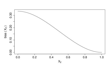
Denote as function , and we have
where . This confounding bias is illustrated in Figure S6.
To compute , we have
where is known. To calculate , we need to figure out the joint distribution of and then the conditional distribution of . Solving the linear system, we get
where , , , and . The conditional PDF should be
Therefore, we have
Similarly, we calculate the for by computing
Therefore,