Evaluating of Machine Unlearning: Robustness Verification Without Prior Modifications
Abstract
Machine unlearning, a process enabling pre-trained models to remove the influence of specific training samples, has attracted significant attention in recent years. While extensive research has focused on developing efficient unlearning strategies, the critical aspect of unlearning verification has been largely overlooked. Existing verification methods mainly rely on machine learning attack techniques, such as membership inference attacks (MIAs) or backdoor attacks. However, these methods, not being formally designed for verification purposes, exhibit limitations in robustness and only support a small, predefined subset of samples. Moreover, dependence on prepared sample-level modifications of MIAs or backdoor attacks restricts their applicability in Machine Learning as a Service (MLaaS) environments. To address these limitations, we propose a novel robustness verification scheme without any prior modifications, and can support verification on a much larger set. Our scheme employs an optimization-based method to recover the actual training samples from the model. By comparative analysis of recovered samples extracted pre- and post-unlearning, MLaaS users can verify the unlearning process. This verification scheme, operating exclusively through model parameters, avoids the need for any sample-level modifications prior to model training while supporting verification on a much larger set and maintaining robustness. The effectiveness of our proposed approach is demonstrated through theoretical analysis and experiments involving diverse models on various datasets in different scenarios.
Index Terms:
Machine unlearning, unlearning verification, machine learning as a service, data reconstruction.I Introduction
Machine unlearning has recently attracted significant attention [1, 2, 3, 4], aiming to selectively remove the influence of specific training samples from trained models. Its growing popularity can be attributed to several factors, including the global trend toward stringent data protection regulations. For example, various legislators have enacted legislation granting individuals the “right to be forgotten,” which requires organizations to unlearn user data upon receiving requests [5]. Prior research on machine unlearning has primarily focused on developing efficient methods for removing specific samples from models. Despite the success achieved in machine unlearning strategies, The verification of unlearning emerged as a new requirement. Verification means a model provider can prove that the requested sample has been removed from the model, or user can test that his/her samples have been unlearned from the model successfully. However, currently, users have limited ability to monitor the unlearning process and confirm if their data has been truly unlearned from the model [1].
Here are some prior research results on the verification of machine unlearning. Weng et al. [6] proposed using trusted hardware to enforce proof of unlearning, though their method relies on trusted execution environments within Machine Learning as a Service (MLaaS). Cao et al. [7] introduced data pollution attacks to assess if the model’s performance was recovered to its original state after the unlearning process. Similarly, Guo et al. [8] evaluated whether the model provider truly performs machine unlearning by analyzing the performance of backdoor attacks. Other verification schemes are based on the distribution of model parameters [9], membership inference attacks (MIAs) [10, 11, 12, 13, 14], model inversion attacks [15, 16], theoretical analysis [17], or model accuracy [18, 19, 20, 21].
However, those unlearning verification schemes have several limitations. Schemes based on model accuracy cannot reliably determine if targeted samples have been truly unlearned, since unlearning partial samples may not significantly affect model performance for those targeted samples [18, 19, 20, 21]. Schemes based on model inversion attacks do not support sample-level verification but rather only enable verification at the class level, as they can only recover class-level representation [15, 16]. Verification schemes, such as those based on MIAs, distribution of model parameters or theoretical analysis, are often ineffective due to unstable performance [11, 12]. Beyond these drawbacks, there are several common limitations:
-
•
Existing unlearning verification schemes always involve modifying samples prior to model training. For example, backdoor-based schemes require altering training samples by adding backdoor triggers [22, 8]. These triggers are then used to verify the unlearning process. Similarly, schemes relying on data pollution use modified, poisoned samples to confirm unlearning. However, if these modifications lose their effect during the learning or unlearning process, those verification schemes become ineffective.
-
•
Most existing unlearning verification methods only support a small, predefined subset of samples. For example, schemes relying on backdoor or data poisoning techniques necessitate the preparation of samples used for verification before model training process. Consequently, those approaches are restricted to verifying only those pre-prepared samples, failing to consider the verification of unlearning for samples that were not modified prior to the training process [22, 8]. This constraint significantly narrows the scope of unlearning verification, potentially leaving critical gaps in the verification process.
-
•
Nearly all existing verification schemes lack robustness, which includes both long-term effectiveness and adaptability to varied-term unlearning conditions. To illustrate the concept of long-term effects, consider verification methods such as those based on parameter distribution, MIAs, backdoor, or data poisoning. These methods may initially demonstrate effectiveness in verifying unlearning immediately after the process. However, their reliability can diminish after subsequent model modifications like fine-tuning or pruning [1, 8, 22]. Moreover, in varied-term scenarios, many verification methods are context-dependent, only confirming successful unlearning under specific, predefined conditions. This limited scope increases the risk of false positives - erroneously confirming successful unlearning when the influence of targeted samples may actually persist or even amplify post-unlearning [23, 24, 14, 25]. (see Section V-E).
In this paper, we propose UnlearnGuard, a novel robustness verification scheme for machine unlearning that operates without requiring any prior modifications to training samples. Our approach is based on the observation that neural networks tend to memorize actual training samples. Therefore, we aim to directly extract these training samples from the model for verification purposes.
-
1.
To address the first limitation, we redefine model training as a maximum margin problem, leveraging insights from implicit bias [26, 27] and data reconstruction [28, 29], we introduce our primary recovery loss component derived from Karush-Kuhn-Tucker (KKT) point conditions. This loss allows us to recover actual training samples from model used for verification without modifying the training samples.
-
2.
To cover as many samples as possible that can be verified for unlearning, we propose an additional loss that allows further recovered samples to exhibit greater similarity to their original counterparts in training data space. This is achieved by minimizing the negative absolute outputs and applying a projection that constrains those newly recovered samples to remain within a specified range of pre-recovered samples. By enhancing this similarity, more recovered samples become suitable for verification.
-
3.
To tackle the limitation of lacking robustness, all proposed loss components only use model parameters for recovery, without incorporating any other information and condition for verification. We also provide theoretical proof based on implicit bias [26, 27], demonstrating how the differences between samples recovered after successful unlearning and those before unlearning, providing a theoretical foundation for robustness property.
It’s worth noting that, in our experiments, we find that some fine-tuning-based machine unlearning schemes does not completely remove the influence of targeted samples. In fact, those schemes appear to deepen the impacts of targeted samples in the model. This result contrasts with previous findings [23, 24, 14, 25]. Comparing with previous verification methods, our proposed verification scheme can further enhance the reliability of machine unlearning.
In summary, we make the following contributions.
-
•
We take the first step in addressing machine unlearning verification problem without prior sample-level modifications, considering both the robustness of the verification scheme and its capacity for more sample verifications.
-
•
We propose an optimization-based method for recovering actual training samples from models, which enables users to verify machine unlearning by comparing samples recovered before and after the unlearning process.
-
•
We provide theoretical proofs and analyses of our scheme based on implicit bias to demonstrate its effectiveness.
II Preliminary
II-A Related Works
II-A1 Machine Unlearning
In response to the right to be forgotten, the machine learning community has proposed various unlearning schemes. In our earlier survey, we comprehensively reviewed recent works on machine unlearning [1]. This survey extensively covered several key aspects, including: (I) the motivation behind machine unlearning; (II) the goals and desired outcomes of the unlearning process; (III) a new taxonomy for systematically categorizing existing unlearning schemes based on their rationale and strategies; and (IV) the characteristics and drawbacks of existing unlearning verification schemes.
Existing machine unlearning schemes are usually based on the following two techniques: data reorganization and model manipulation [1]. Data reorganization refers to restructuring the training dataset to facilitate efficient machine unlearning. Cao et al. [7] transformed the training dataset into summations forms, allowing updates to summations rather than retraining the entire model. Bourtoule et al. [4] proposed one “Sharded, Isolated, Sliced, and Aggregated” (SISA) framework, where data is partitioned into disjoint shards, and sub-models are retrained only on the shards containing the sample to be unlearned. Similar schemes are used in graph tasks [3]. Model manipulation-based schemes usually adjust the model’s parameters directly. Guo et al. [17] proposed a certified removal scheme based on the influence function [30] and differential privacy [31]. Schemes in [32, 33] consider unlearning requests in federated learning setting. Kurmanji et al. [12] and Chen et al. [34] use machine unlearning techniques to address bias issues and resolve ambiguities or confusion in machine learning models.
II-A2 Machine Unlearning Verification
Current schemes for verifying machine unlearning can be broadly categorized into: empirical evaluation and theoretical analysis [1].
Empirical evaluation schemes mainly employ attack methods to evaluate how much information about samples targeted for unlearning remains within the model. For example, model inversion attacks have been used in studies, such as [15, 16], while membership inference attacks (MIAs) were employed in [11, 12, 13, 14]. Cao et al. [7] introduced data pollution attacks to verify whether the model performance was restored to its initial state after the unlearning process. Similar strategies involving backdoor attacks were adopted in [35, 22, 8]. Beyond attack-based methods, Liu et al. [9], Wang et al. [21] and Brophy et al. [20] used accuracy metrics, whereas Baumhauer et al. [4], Golatkar et al. [36, 19], and Liu et al. [37] measured the similarity of distributions of pre-softmax outputs. Additionally, some efforts have been made to compare the similarity between the parameter distributions of a model after unlearning and a model after retraining from scratch [9]. On the other hand, theoretical analysis schemes typically focus on ensuring that the unlearning operation effectively removes the targeted sample information from model [17].
II-A3 Discussion of Related Works
Despite the progress made in machine unlearning, current verification methods still face significant challenges. The limitations of existing verification schemes can be summarized as follows:
- •
-
•
Similarity-Based Verification: Approaches that measure the similarity of distributions, such as pre-softmax outputs or parameters, have been shown to be ineffective in [38].
-
•
Attack-Based Verification: Schemes based on model poisoning attacks, such as data pollution [7] and backdoor attacks [35, 22, 8] require modification of a subset of samples before model training. Consequently, those methods can only verify the unlearning process for specific samples that were poisoned during training, but not for any unspecified data after training.
-
•
Theoretical Analysis Verification: While theoretical analysis schemes [17] can ensure the unlearning results, they are often constrained by specific unlearning strategies and are less effective with complex models and large datasets.
Most importantly, the majority of existing verification methods, including data pollution [7] and backdoor attack-based [35, 8], fail to consider long-term verification. While these methods may be effective immediately after unlearning, they become invalid once the model undergoes a fine-tuning or pruning process. We will discuss this in detail in Section III-A.
II-B Background
Machine Learning as a Service (MLaaS) primarily involves two key entities: the data provider and the model provider. The data provider submits their data to the model provider, who then uses this data for model training. We denote the dataset of the data provider as , where each sample is a -dimensional vector, is the corresponding label, and is the size of . Let be a (randomized) learning algorithm that trains on and outputs a model . The model is given by , where and is the hypothesis space. After the training process, data providers may wish to unlearn specific samples from the trained model and submit an unlearning request. Let represent the subset of the training dataset that the data provider wishes to unlearn. The complement of this subset, , represents the data that the provider wishes to retain.
Definition 1 (Machine Unlearning [1])
Consider a set of samples that a data provider wishes to unlearn from an already-trained model, denoted as . The unlearning process, represented as , is a function that takes an already-trained model , the training dataset , and the unlearning dataset , and outputs a new model . This process ensures that the resulting model, , behaves as if it had never been trained on .
After the machine unlearning process, a verification procedure is employed to determine whether the requested samples have been successfully unlearned from the model. Typically, data providers lack the capability to perform this verification independently. For example, verification schemes based on MIAs often require the training of attack models using multiple shadow models, which can be too resource-intensive for data providers. Consequently, verification operations in MLaaS are usually conducted by a trusted third party. With the assistance of this trusted third party, a distinguishable check will be conducted to ensure that .
III Problem Definition
III-A Existing Verification Schemes
Designing an effective and efficient verification scheme for machine unlearning is difficult. As discussed in Section II-A2, verification schemes based on accuracy, theoretical analysis and distribution similarity have consistently proven ineffective in [1, 38]. In this Section, we further highlight the critical limitations of attack-based verification schemes to illustrate the novelty of our scheme. Figure 1 illustrates the main ideas of commonly used attack-based verification schemes.
As shown in Figure 1, attack-based unlearning verification schemes typically involve three roles, including data provider, model provider and one trusted third party. Data provider first pre-selects a subset of triggers before model training. For example, in schemes based on data pollution and backdoor attacks, triggers are often generated by a trusted third party [7, 35, 8]. In MIAs-based verification schemes, data providers directly select partial training samples as those triggers [11, 12, 13, 14]. Based on those triggers, the verification process can be summary as the following steps:
-
•
Trigger Integration: Triggers , either generated from a trusted third party or selected directly from the data provider’s own dataset, are added to the training dataset. The model is then trained on this combined dataset.
-
•
Initial Prediction: The data provider sends the verification request to the trusted third party, and the trusted third party queries the model’s prediction for these triggers. The model provider returns the predictions . Existing attack-based verification scheme outputs the verification result for based on .
-
•
Unlearning Request: The data provider submits an unlearning request for those triggers .
-
•
Post-Unlearning Prediction: The data provider and the trusted third party repeat the steps in the initial prediction phase and output the verification result .
-
•
Verification: By comparing the returned predictions before and after unlearning, and respectively, the data provider determines if the model has undergone the unlearning process.

However, those attack-based machine unlearning verification schemes mainly have the following limitations:
-
•
Sample-Level Modification before Model Training: Ensuring effective verification often requires incorporating a large number of modified samples, such as backdoored samples, which increases computational costs.
-
•
Support Only a Small, Predefined Subset of Samples: Some schemes use pre-embedded patterns for verification, like backdoor triggers, limiting the process to only those samples. This means the number of verifications must be considered before training, and once these samples are used up, no further verification is possible.
-
•
Lacking Robustness Verification: These schemes focus solely on verifying the unlearning process immediately and lack robustness, meaning the model cannot be fine-tuned or pruned for new demands after unlearning.
-
•
Model Performance Degradation and Security Risks: Verification schemes based on data pollution and backdoor attacks rely on poisoned samples, inheriting the drawbacks of poisoning methods. This can harm model performance and introduce security risks, limiting their adoption for verification.
III-B Threat Model and Goals
In MLaaS, there are two main roles: data providers and model providers. Data providers also act as verifiers of unlearning, while model providers are responsible for executing it. The data provider shares its dataset with the model provider, who trains a model using a learning algorithm. After training, beyond making regular predictions, the data provider can submit unlearning requests to remove their data from the model. However, model providers may not always be fully trustworthy in performing unlearning, either because this process is time-consuming, or large-scale unlearning requests could negatively impact model performance [8, 35]. The background and goals of data providers are as follows:
-
•
Background: Data providers only have the ability to upload their training data or send prediction, unlearning requests to the model providers.
-
•
Goal: After submitting the unlearning request, data providers want to confirm whether their data has been truly unlearned from the model.
Meanwhile, the background and goals of model providers are as follows:
-
•
Background: Model provider can collect training data from the data provider and train the model.
-
•
Goal: After receiving the unlearning requests from data provider, model providers prefer to avoid executing unlearning as much as possible to protect their own interests.
This paper proposes a method for data providers to verify whether their samples have been successfully unlearned from the trained model. Specifically, we have four aims related to machine unlearning verification.
-
•
No Pre-defined Modifications: Develop a verification scheme that enables data providers to confirm the execution of the unlearning process without depending on any pre-defined sample-level modifications.
-
•
More Sample Coverage: Design a scheme supporting unlearning verification for nearly all samples involved in the training process.
-
•
Robustness Verification: Address the need for robustness by supporting immediate post-unlearning verification and enabling verification in scenarios where the model undergoes further changes after unlearning (e.g., further fine-tuning or model pruning).
-
•
Preserving Model Usability: Ensure that the verification scheme does not negatively impact: model performance, security, and training efficiency.
We assume that the data provider conducts verification with the help of a trusted third party. This assumption reflects real-world MLaaS scenarios where data providers often lack the capability to independently verify the unlearning processes [8]. The trusted third party is granted access to the trained model for verification purposes upon receiving unlearning requests. Additionally, we assume that the model provider may carry out further model modifications (e.g., fine-tuning and pruning) after executing the unlearning process.

IV Methodology
IV-A Overview
Current unlearning verification schemes typically depend on additional information to verify the unlearning process, such as pre-embedded backdoors [8, 35]. However, these schemes become ineffective if this additional information is disrupted during subsequent model fine-tuning or pruning. Therefore, it is crucial to verify the unlearning process only using the model itself and investigate if the information can still be recovered from the model parameters post-unlearning.
In this paper, we propose a robustness verification scheme without prior modifications, named UnlearnGuard, which verifies machine unlearning based only on the model and possesses robustness properties. As illustrated in Figure 2, UnlearnGuard directly verifies the unlearning process by examining whether the model parameters contain information about the unlearning samples. Before and after unlearning, the data provider sends a verification request about to trusted third party. The trusted third party ask model from model provider and attempts to recover from it. Based on two recovery results, the data provider can determine if the data was truly unlearned. Our approach distinguishes UnlearnGuard from the scheme illustrated in Figure 1 as UnlearnGuard relies only on the model itself rather than any prior sample-level modifications.
We describe our scheme based on the following two subsections: unlearning verification process and sample recovery process. In Section IV-B, we introduce the main workflow of our entire unlearning verification process, which includes the pre-unlearning process and the post-unlearning process, encompassing all steps shown in Figure 2. Next, in Section IV-C, we explain how to recover actual unlearning samples from the model, which is the most important part of our scheme and supports the workflow of Section IV-B.
IV-B Unlearning Verification Process
In this section, we will describe the whole workflow of our unlearning verification process, including three steps.
IV-B1 Model Training and Pre-verification
Data providers can submit their datasets to MLaaS for model training, enhancing accessibility and efficiency in machine learning deployment. After training, with the help of a trusted third party, data providers can perform pre-verification to confirm the presence of their data within the trained model. While this verification step enhances the comprehensiveness of our proposed scheme, it is not mandatory for practical implementations.
To conduct this, data providers send sample to a trusted third party, requesting confirmation of ’s presence in the model. The trusted third party then asks the MLaaS model provider for the trained model and attempts to recover the samples using the scheme described in Section IV-C. This verification process outputs a result .
IV-B2 Unlearning Request and Execution
To initiate unlearning, the data provider sends a request regarding samples . The model provider locates and removes sample from the dataset and executes the unlearning process.
IV-B3 Re-query and Verification
Following the unlearning request, the data provider again inquires about ’s presence in the model. The trusted third party returns the output , where represents the updated model after unlearning. The data provider then compares and to determine whether the model provider has successfully executed the unlearning operation. In Algorithm 1, we provide a detailed process for this process.
In Algorithm 1, lines 2-3, denote the pre-verification process. Specially, the initial result should be True. Line 4 shows the data provider sending an unlearning request, followed by another query for the result related to (lines 5-6). If is False, it confirms that the model provider has truly executed the unlearning operation (lines 7-8); otherwise, it suggests that the model provider has not executed the unlearning operation (lines 9-10). In our scheme, we define the function as:
| (1) |
where denotes the logical OR operation and is the number of recovered samples.
IV-C Sample Recovery Process
In the previous section, we explained the process of verifying unlearning, mainly based on comparing the recovery results before and after unlearning. This section describes how to recover actual training samples encoded within a trained model, leveraging implicit bias and date reconstruction.
We begin by studying simple models before advancing to the analysis of more complex deep models in Section IV-D. Let be a binary classification training dataset. Consider a neural network : parameterized by . For a given loss function , the empirical loss of on the dataset is given by: . Let us consider the logistic loss, also known as binary cross-entropy, which is defined as .
Directly recovering samples from the above-defined model poses significant challenges. To address this, we reformulate model training problem into a maximum margin problem based on the implicit bias theory discussed by Ji et al. [26] and Lyu et al. [27], which simplifies the process of recovering samples from the model.
Theorem 1 (Paraphrased from Ji et al. [26], Lyu et al. [27]): Consider a homogeneous neural network . When minimizing the logistic loss over a binary classification dataset using gradient flow, and assuming there exists a time such that , then, gradient flow converges in direction to a first-order stationary point of the following maximum-margin problem:
| (2) |
In this theorem, homogeneous networks are defined with respect to their parameters . Specifically, a network is considered homogeneous if there exists such that for any , and , the relationship holds. This means that scaling the parameters by any factor results in scaling the outputs by . Gradient flow is said to converge in the direction to if , where is the parameter vector at time . means that there exists time at which the network classifies all the samples correctly.
This theorem describes how optimization algorithms, such as gradient descent, tend to converge to specific solutions that can be formalized as Karush-Kuhn-Tucker (KKT) conditions, enabling data reconstruction from the model using those conditions [28]. The reconstruction loss can be defined as following. Derivation details can be found in Section IV-D.
| (3) | ||||
| s.t. | ||||
where denotes the cardinality of the sample set to be reconstructed, typically set to in their experimental setting. The loss represents the stationarity condition satisfied by the parameters at the KKT point, while represents the dual feasibility condition. denotes some supplementary constraints predicated on image attributes, such as ensuring pixel values remain between .
Using the above can recover the actual sample from the model, which is our main purpose. However, only using this loss to reconstruct samples exhibits limitations in the context of partial verification. Specifically, it is constrained to reconstructing only those training samples that almost lie on the decision boundary margin. Consequently, when employed to verify the unlearning process, its efficacy is limited to a subset of samples—those situated on the margin. To expand the scope of reconstruction, we introduce a novel loss term, denoted as the prior information loss, .
The introduction of this new loss term aims to incorporate classification information pertaining to the samples targeted for recovery. Let represent the samples recovered based on the aforementioned scheme. Our objective is to ensure that the subsequently recovered samples exhibit greater similarity to their counterparts in the training data space:
| (4) |
Specifically, we aim to maximize assigned to the predicted class for each sample by minimizing its negative absolute value. It is noteworthy that this optimization process does not utilize the original labels. Instead, it optimizes the model’s output confidence (logits) for samples , aligning with our hypothesis of implementing unlearning verification using only the model parameters.
Finally, we define our recovery loss as:
| (5) | ||||
| s.t. | ||||
where we eliminate the loss term and incorporate to enhance the fidelity of recovered samples.
To mitigate excessive deviation of the newly recovered samples from in the data space, we introduce a projection function, project_to_bounds, applied after each optimization epoch. This function constrains the pixel values of to within the range . Our recovery algorithm is shown in Algorithm 2.
In lines 1-3, we initially optimize and utilizing the loss . This preliminary phase ensures that achieves a basic level of recovery. Subsequently, we proceed to optimize further to recover samples using the augmented loss function (lines 5-8). At each optimization epoch, we project the recovered samples onto a constrained space (line 8). This ensures they remain within a specified range of the pre-recovered samples while capturing more essential features required for effective unlearning verification.
IV-D Theoretical Analysis
Our machine unlearning verification scheme builds upon existing works [27, 26, 28, 29], extending their insights to the context of machine unlearning. We provide a rigorous theoretical basis for our verification method, incorporating concepts from optimization theory and functional analysis.
Let be a binary classification training dataset. Consider a neural network : parameterized by . The training process with a logistic loss can be viewed as an implicit margin maximization problem.
As we discussed in Theorem 1, for a homogeneous ReLU neural network , gradient flow on the logistic loss
| (6) |
converges in direction to a KKT point of:
| (7) |
subject to
| (8) |
| (9) |
Based on these KKT conditions, we can formulate a reconstruction method [28, 29]. The goal is to find a set of and that satisfy following equation:
| (10) |
where:
| (11) |
| (12) |
Let be an unlearning operator that unlearns from a model with parameters to :
| (13) |
To verify unlearning, we compare the recovered samples before and after unlearning those samples. Let be the index set of samples to be unlearned. The parameters of the model after unlearning should also satisfy the KKT conditions:
| (14) |
And the corresponding is
| (15) |
where:
| (16) |
| (17) |
The verification involves:
-
1.
Performing sample recovery on both the original model and the unlearned model , obtaining recovery samples sets and .
-
2.
Calculating the differences between recovered samples:
(18) -
3.
Comparing the differences for samples that unlearned and retained samples:
(19)
If the unlearning process is effective, we expect:
| (20) |
This expectation arises because:
- 1.
- 2.
Additionally, recent work proposed by Buzaglo et al. [29] has extended the reconstruction method in [28] to multi-class classification scenarios. For a dataset , where is the number of classes, and a neural network : . Then, the KKT conditions for the multi-class problem yield:
| (21) |
The corresponding loss can be formulated as:
| (22) |


In this case, the above-proof process is also applicable. We will use this loss in our experimental evaluation when dealing with multi-classification tasks.
This theoretical framework utilizes the implicit bias inherent in neural network training and Karush-Kuhn-Tucker (KKT) conditions of margin maximization to evaluate the unlearning process. By analyzing the difference between recovered samples before and after the unlearning process, we can determine if the model provider has successfully removed the targeted samples from the model.
V Performance Evaluation
V-A Experiment Setup
To evaluate our scheme, we utilize four widely-used image datasets: MNIST111http://yann.lecun.com/exdb/mnist/, Fashion MNIST222http://fashion-mnist.s3-website.eu-central-1.amazonaws.com/, CIFAR-10333https://www.cs.toronto.edu/ kriz/cifar.html and SVHN444http://ufldl.stanford.edu/housenumbers/.
V-A1 Baseline Methods
We compare our scheme against the following established methods:


V-A2 Metrics
We consider the following metrics to separately evaluate the baseline scheme and our scheme:
-
•
For membership inference attacks-based scheme [39], we use the success rate of attacking samples as our metric, defined as where is the number of samples predicted to be in the training set, and is the total tested samples. Ideally, should be close to before unlearning and approach after unlearning.
- •
-
•
For model inversion attack-based scheme [15], we directly show the recovered samples. Ideally, before unlearning, those samples should contain discernible information about the class targeted for unlearning. After unlearning, Those samples should appear dark, jumbled, and dissimilar from the unlearning class, indicating the successful unlearning of class-specific information.
-
•
For our scheme, we evaluate it using both qualitative and quantitative perspectives. Qualitative: visual inspection of recovered samples, similar to the model inversion attack-based schemes. Quantitative: we use the SSIM to evaluate the similarity between recovered and original unlearning samples. SSIM values range from to , with higher values indicating greater similarity.


V-B Verification Results
Our evaluation includes sample and class level unlearning requests. To ensure consistency with existing studies [8], we employ retraining from scratch as our unlearning method.
V-B1 Sample-Level Unlearning Verification
Figure 3 and 4 show our experimental results. Figure 3 illustrates the results for unlearning samples before and after the unlearning process, while Figure 4 shows results for samples not unlearned. Each sub-figure demonstrates the performance of various verification schemes across different datasets. The Y-axis represents different metrics depending on the scheme: INA for membership inference attacks (MIAs)-based schemes, ASR for backdoor-based schemes, accuracy for accuracy-based schemes, and SSIM for our proposed verification scheme. The conclusion can be summary as follows:
-
•
MIAs-based and Accuracy-based Schemes: Before unlearning, success rates for identifying both unlearning and remaining samples are high, indicating that MIAs effectively identify samples used in model training. However, after unlearning, there’s no significant reduction in attack performance for either sample type. This suggests that MIAs cannot reliably distinguish whether training samples have been successfully unlearned. Similar results can be observed from the results of accuracy-based schemes.
-
•
Backdoor-based Scheme: Following backdoor embedding, the accuracy of classifying both unlearning and remaining samples as targets is very high. After unlearning, the classification accuracy for unlearning samples with the backdoor drops to nearly , while remaining higher for other samples. This indicates that the backdoor-based verification scheme effectively confirms the unlearning process, demonstrating the successful removal of backdoor samples associated with unlearning.
-
•
Our Proposed Scheme: Prior to unlearning, all recovered samples show high similarity based on the SSIM metric. After the unlearning process, SSIM values for unlearning samples decrease significantly, while remaining high for other samples. Those SSIM values before and after unlearning demonstrate that our scheme effectively distinguishes between unlearned and retained samples.


We also show some original training samples and recovered samples extracted using our scheme in Figure 5. Each column shows unlearning samples on the left and the remaining samples on the right. Before unlearning, our scheme effectively recovers all samples. After unlearning, the samples that were most similar to those samples targeted for unlearning no longer contained relevant information, while for the remaining samples, our scheme still recovers images similar to the originals. This demonstrates our scheme’s ability to effectively distinguish between unlearned and retained samples, validating it can be used as a verification method.
V-B2 Class-Level Unlearning Verification
We set the remaining class to for the MNIST dataset and to for the FashionMNIST dataset. The unlearning class is selected as for both datasets. Figure 6 shows the quantitative results of our evaluation. Specifically, Figure 6(a) and Figure 6(c) show the results for the unlearning class and the remaining class in the MNIST dataset, while Figure 6(b) and Figure 6(d) illustrate the changes in the unlearning class and the remaining class for the FashionMNIST dataset.


Results. For samples in the class that need to be unlearned, MIA-based, accuracy-based, and our proposed methods all show significant changes (see Figures 6(a) and 6(b)). For remaining class, no significant changes are observed across all three approaches (see Figures 6(c) and 6(d)). This indicates that all methods are effective for class-level unlearning verification.
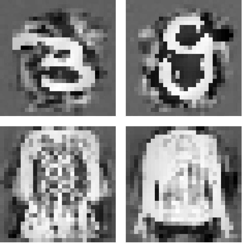
Figure 7 and 8 show some original and recovered samples extracted using the model inversion attack-based scheme and our scheme. In Figure 7, before unlearning, the model inversion attack reconstructs representatives containing information about the unlearning class. After unlearning, it produces dark, jumbled images with almost no information about the unlearning class. Similarly, for our scheme, the recovered sample after unlearning all samples in the unlearning class also becomes dark and jumbled, which illustrates that our scheme can also be used in verifying class-level unlearning requests.
Summary. The above experiments demonstrate that the proposed verification scheme effectively validates both sample-level and class-level unlearning requests. The method consistently performs well across these different granularity levels, showcasing its applicability and reliability in various scenarios.
V-C Robustness Evaluation
As highlighted in Section III-A, the robustness of unlearning verification scheme is crucial for long-term deployment. A robust verification scheme should remain effective even after fine-tuning or pruning the models when the training or unlearning process is finished. In this Section, we evaluate the robustness of our proposed scheme, comparing it with the backdoor-based verification scheme [22]. We use the same experimental settings described in Section V-B1 and re-evaluate these schemes after performing the following operations:
-
(1)
Training model Pruning model
-
(2)
Training model Fine-tuning model
-
(3)
Training model Unlearning Fine-tuning model
For pruning, we randomly prune of the parameters in each layer. For fine-tuning, we train the model using the original training samples and correct labels, maintaining the initial training configuration. For unlearning, we use retraining from scratch [8]. The results of the backdoor-based scheme are illustrated in Figure 9, while Figure 10 presents the results of our proposed scheme.


Results: As shown in Figure 9(a), when the model undergoes pruning after training, the backdoor-based verification scheme becomes ineffective, as evidenced by the near-zero performance on the poison dataset. This indicates that the backdoor-based verification loses its robustness in the face of pruning operations, rendering it unusable. Similarly, in Figure 9(b), when fine-tuning is performed using the original, unperturbed training samples, the accuracy of the backdoor also decreases, indicating that fine-tuning also compromises the robustness of the backdoor-based verification scheme. Lastly, Figure 9(c) illustrates that when the model is finetuned with previously unlearned samples after unlearning, the backdoor-based verification scheme also fails due to the absence of the backdoor pattern in those samples. In conclusion, the backdoor-based method relies on pre-prepared samples for verification. If the backdoor pattern is not embedded in advance, if those patterns are disrupted after training, or if the backdoor has been previously used, subsequent verification will be infeasible.
Figure 10 shows the results obtained from our scheme. Figure 10(a) illustrate the original training sample, while other Figures show samples recovered after various processes: initial training (Figure 10(b)), pruning (Figure 10(c)), fine-tuning (Figure 10(d)), and unlearning followed by fine-tuning (Figure 10(e)). Unlike the backdoor-based scheme, our scheme effectively recovers training samples even after the model has been subjected to these modifications. This consistent performance demonstrates that our method exhibits a higher degree of robustness, maintaining its effectiveness across various post-training adjustments where the backdoor-based scheme fails.


Summary. The above experiments demonstrate that, as the backdoor-based verification scheme depends on pre-prepared patterns for verification, if those pre-prepared patterns are not embedded in advance, are disrupted after training, or have been previously used, subsequent verification becomes infeasible. In contrast, our method demonstrates consistent performance and a higher degree of robustness, maintaining effectiveness across various post-training adjustments.
V-D Ablation Study and Analysis of Verification Range
As discussed in Section III-A, the ability to verify more samples is crucial in MLaaS unlearning verification. This section evaluates the number of verifications supported by our proposed scheme compared to the method introduced in [22]. Furthermore, in Section IV-C, we add a new constraint to improve the quality of recovered samples and provide more samples used for unlearning verification. In this Section, we also do a comparative analysis between our enhanced scheme and the data reconstruction scheme proposed in [29].
We follow experimental settings used in [29] to construct our comparison experiment. Specifically, we use the experimental setting in V-B1 and select the MNIST dataset. We first recover samples based on the loss and record the result as original. Then we add our new loss to and continue to recover samples. We set , and and record the recover samples as ours. We adopted the same other hyperparameters provided in [29]. To evaluate the quality of our recovered samples, we employ the same evaluation method in [29]: for each sample in the original training dataset we search for its nearest neighbor in the recovered samples and measure the similarity using SSIM. A higher SSIM value indicates better recovery quality. In Figure 11(a), we plot the recovery quality (measured by SSIM) against the sample’s distance from the decision boundary. This distance is calculated based on:
where is the logit for the true class, and is the maximum logit among all other classes. In Figure 11(b), we show the change of SSIM for each corresponding original sample. For the backdoor-based scheme [22], we choose the experimental setting in V-B1 and use the same number of the training dataset in Buzaglo et al. [29]. The corresponding results are shown in Figure 11(c).


Results. Figures 11(a) demonstrates that both schemes proposed in [29] and ours successfully recover various samples from the model, aligning with the findings reported in [29]. In addition, our scheme shows an improvement, with a larger proportion of recovered samples (blue points) exhibiting greater similarity to the training dataset compared to the original scheme (red points) in Figure 11(a). Figure 11(b) visually represents this improvement, with green arrows indicating samples where our scheme achieves higher similarity, gray points representing unchanged similarity, and red arrows denoting decreased similarity. This improved similarity between recovered samples and training samples provides more samples for our subsequent verification processes.


Additionally, as shown in Figure 11(c), when the proportion of backdoored samples used for training is less than , their performance is inadequate for unlearning verification. Effective verification is achieved only when the proportion of backdoored samples reaches . This suggests that, for the MNIST dataset, approximately of the total training samples (500 in total) is necessary for a single verification. Given the total number of samples, it only supports times for verification. Furthermore, as the number of backdoored samples increases, the model’s performance will significantly decrease since the samples that have not been backdoored become less. For example, from Figure 11(c), when only training samples for original task training, the performance of the trained model will decrease to only . For our scheme, we show some recovered samples in Figure 12. It can be seen that when the SSIM of the recovered image equals , the recovered samples still partially retain information about the original sample. From Figure 11(a), we observe that approximately samples have an SSIM greater than . This suggests that our scheme can support over times the number of verifications compared to backdoor-based methods, without compromising the model’s original performance.
Summary. Our enhanced sample recovery method significantly improves the quality of samples available for verification. In addition, it also allows a substantially higher number of verifications compared to existing backdoor-based methods, while maintaining model’s performance on its primary task.
V-E Fine-tuning is not a Solution
Currently, many machine unlearning schemes achieve their goals through fine-tuning process [1]. This typically involves manipulating the samples targeted for unlearning, such as assigning random labels, and then fine-tuning the model with those relabeled samples [23, 24, 14, 25]. Experimental evaluations in these works, using membership inference attacks, model inversion attacks, backdoor attack and accuracy-based metrics, have suggested successful unlearning. However, the question remains: Is this truly the case?
Intuitively, any fine-tuning-based unlearning scheme involving unlearning samples should be considered incomplete, as samples targeted for unlearning are still processed by the model during the fine-tuning stage. To verify this hypothesis, we used the experimental setting described in Section V-B2, focusing on the MNIST dataset and replacing the unlearning method with relabel-based fine-tuning [14, 25]. We use our proposed scheme to recover samples both before and after fine-tuning. For evaluation, we select all recovered samples that can be correctly classified as class targeted for unlearning using the model before unlearning. Then, we calculate the SSIM between each recovered sample and its nearest original sample. Figure 13 shows the SSIM results, while Figure 14 shows some recovered samples after fine-tuning.
Results. As shown in Figure 13(a), before performing relabel-based finetuning, the SSIM between some recovered samples and training samples is very high, indicating that the trained model indeed contains some information about the class that needs to be unlearned. Figure 13(b) also reveals similar results, with many recovered samples exhibiting high similarity to the training samples (see both recovered samples in Figure 14). Furthermore, after fine-tuning, the number of recovered samples unexpectedly increases, as the model retains memory not only of the original training samples but also of the newly added fine-tuning samples. All those results suggest that even after unlearning, the model still retains information about the samples that need to be unlearned. Therefore, relabel-based fine-tuning is not an effective unlearning solution.
VI Conclusion
In this paper, we introduce a novel approach to machine unlearning verification, addressing the challenges of prior sample-level modifications while considering both robustness and supporting verification on a much larger set. Inspired by the existing works in implicit bias and date reconstruction, we propose an optimization-based method for recovering actual training samples from models. This enables verification of unlearning by comparing samples recovered before and after the unlearning process. We provide theoretical analyses of our scheme’s effectiveness. Experimental results demonstrate robust verification capabilities while supporting verify a large number of samples, marking a significant advancement in machine unlearning research. In addition, our machine unlearning verification scheme revealed that relabeling fine-tuning methods do not fully remove, but rather amplify, the influence of targeted samples, challenging previous findings. This suggests that our verification scheme can further enhance the reliability of machine unlearning.
References
- [1] H. Xu, T. Zhu, L. Zhang, W. Zhou, and P. S. Yu, “Machine unlearning: A survey,” ACM Comput. Surv., vol. 56, no. 1, pp. 9:1–9:36, 2024.
- [2] D. Ye, T. Zhu, C. Zhu, D. Wang, K. Gao, Z. Shi, S. Shen, W. Zhou, and M. Xue, “Reinforcement unlearning,” in NDSS, 2025.
- [3] M. Chen, Z. Zhang, T. Wang, M. Backes, M. Humbert, and Y. Zhang, “Graph unlearning,” in CCS, 2022, pp. 499–513.
- [4] L. Bourtoule, V. Chandrasekaran, C. A. Choquette-Choo, H. Jia, A. Travers, B. Zhang, D. Lie, and N. Papernot, “Machine unlearning,” in 42nd IEEE Symposium on Security and Privacy, 2021, pp. 141–159.
- [5] “General Data Protection Regulation (GDPR),” 2018.
- [6] J. Weng, S. Yao, Y. Du, J. Huang, J. Weng, and C. Wang, “Proof of unlearning: Definitions and instantiation,” IEEE Trans. Inf. Forensics Secur., vol. 19, pp. 3309–3323, 2024.
- [7] Y. Cao and J. Yang, “Towards making systems forget with machine unlearning,” in 2015 S&P, 2015, pp. 463–480.
- [8] Y. Guo, Y. Zhao, S. Hou, C. Wang, and X. Jia, “Verifying in the dark: Verifiable machine unlearning by using invisible backdoor triggers,” IEEE Trans. Inf. Forensics Secur., vol. 19, pp. 708–721, 2024.
- [9] Y. Liu, L. Xu, X. Yuan, C. Wang, and B. Li, “The right to be forgotten in federated learning: An efficient realization with rapid retraining,” in IEEE INFOCOM, London, May 2-5, 2022, pp. 1749–1758.
- [10] G. Liu, T. Xu, X. Ma, and C. Wang, “Your model trains on my data? protecting intellectual property of training data via membership fingerprint authentication,” IEEE TIFS., vol. 17, pp. 1024–1037, 2022.
- [11] J. Jia, J. Liu, P. Ram, Y. Yao, G. Liu, Y. Liu, P. Sharma, and S. Liu, “Model sparsity can simplify machine unlearning,” in NeurIPS, 2023.
- [12] M. Kurmanji, P. Triantafillou, J. Hayes, and E. Triantafillou, “Towards unbounded machine unlearning,” in NeurIPS, 2023.
- [13] J. Foster, S. Schoepf, and A. Brintrup, “Fast machine unlearning without retraining through selective synaptic dampening,” in Thirty-Eighth AAAI Conference on Artificial Intelligence, AAAI, 2024, pp. 12 043–12 051.
- [14] M. Chen, W. Gao, G. Liu, K. Peng, and C. Wang, “Boundary unlearning: Rapid forgetting of deep networks via shifting the decision boundary,” in CVPR. IEEE, 2023.
- [15] L. Graves, V. Nagisetty, and V. Ganesh, “Amnesiac machine learning,” in AAAI, 2021, pp. 11 516–11 524.
- [16] V. S. Chundawat, A. K. Tarun, M. Mandal, and M. S. Kankanhalli, “Zero-shot machine unlearning,” IEEE Trans. Inf. Forensics Secur., vol. 18, pp. 2345–2354, 2023.
- [17] C. Guo, T. Goldstein, A. Y. Hannun, and L. van der Maaten, “Certified data removal from machine learning models,” in ICML, 2020.
- [18] A. Golatkar, A. Achille, and S. Soatto, “Forgetting outside the box: Scrubbing deep networks of information accessible from input-output observations,” in ECCV, vol. 12374, 2020, pp. 383–398.
- [19] A. Golatkar, A. Achille, A. Ravichandran, M. Polito, and S. Soatto, “Mixed-privacy forgetting in deep networks,” in CVPR, 2021.
- [20] J. Brophy and D. Lowd, “Machine unlearning for random forests,” in ICML 2021, 18-24 July 2021, Virtual Event, ser. Proceedings of Machine Learning Research, vol. 139. PMLR, 2021, pp. 1092–1104.
- [21] J. Wang, S. Guo, X. Xie, and H. Qi, “Federated unlearning via class-discriminative pruning,” in WWW ’22: The ACM Web Conference 2022, Virtual Event, Lyon, France, April 25 - 29. ACM, 2022, pp. 622–632.
- [22] Y. Li, M. Zhu, X. Yang, Y. Jiang, T. Wei, and S. Xia, “Black-box dataset ownership verification via backdoor watermarking,” IEEE Trans. Inf. Forensics Secur., vol. 18, pp. 2318–2332, 2023.
- [23] H. Xu, T. Zhu, L. Zhang, W. Zhou, and P. S. Yu, “Update selective parameters: Federated machine unlearning based on model explanation,” CoRR, vol. abs/2406.12516, 2024.
- [24] A. K. Tarun, V. S. Chundawat, M. Mandal, and M. Kankanhalli, “Fast yet effective machine unlearning,” IEEE Transactions on Neural Networks and Learning Systems, pp. 1–10, 2023.
- [25] H. Chen, T. Zhu, X. Yu, and W. Zhou, “Machine unlearning via null space calibration,” in IJCAI-24, 8 2024, main Track.
- [26] Z. Ji and M. Telgarsky, “Directional convergence and alignment in deep learning,” in NeurIPS, 2020.
- [27] K. Lyu and J. Li, “Gradient descent maximizes the margin of homogeneous neural networks,” in ICLR, 2020.
- [28] N. Haim, G. Vardi, G. Yehudai, O. Shamir, and M. Irani, “Reconstructing training data from trained neural networks,” in NeurIPS, 2022.
- [29] G. Buzaglo, N. Haim, G. Yehudai, G. Vardi, Y. Oz, Y. Nikankin, and M. Irani, “Deconstructing data reconstruction: Multiclass, weight decay and general losses,” in NeurIPS, 2023.
- [30] P. W. Koh and P. Liang, “Understanding black-box predictions via influence functions,” in ICML, 2017.
- [31] T. Zhu, G. Li, W. Zhou, and P. S. Yu, “Differentially private data publishing and analysis: A survey,” IEEE Trans. Knowl. Data Eng., vol. 29, no. 8, pp. 1619–1638, 2017.
- [32] L. Zhang, T. Zhu, H. Zhang, P. Xiong, and W. Zhou, “Fedrecovery: Differentially private machine unlearning for federated learning frameworks,” IEEE Trans. Inf. Forensics Secur., vol. 18, pp. 4732–4746, 2023.
- [33] Y. Lin, Z. Gao, H. Du, D. Niyato, J. Kang, and X. Liu, “Incentive and dynamic client selection for federated unlearning,” in WWW, 2024.
- [34] R. Chen, J. Yang, H. Xiong, J. Bai, T. Hu, J. Hao, Y. Feng, J. T. Zhou, J. Wu, and Z. Liu, “Fast model debias with machine unlearning,” in NeurIPS, 2023.
- [35] D. M. Sommer, L. Song, S. Wagh, and P. Mittal, “Athena: Probabilistic verification of machine unlearning,” Proc. Priv. Enhancing Technol., vol. 2022, no. 3, pp. 268–290, 2022.
- [36] A. Golatkar, A. Achille, and S. Soatto, “Eternal sunshine of the spotless net: Selective forgetting in deep networks,” in CVPR, 2020.
- [37] G. Liu, X. Ma, Y. Yang, C. Wang, and J. Liu, “Federaser: Enabling efficient client-level data removal from federated learning models,” in 29th IEEE/ACM IWQOS, Tokyo, June 25-28, 2021, 2021, pp. 1–10.
- [38] A. Thudi, H. Jia, I. Shumailov, and N. Papernot, “On the necessity of auditable algorithmic definitions for machine unlearning,” in 31st USENIX Security, Boston, USA, August 10-12, 2022, pp. 4007–4022.
- [39] Y. Liu, R. Wen, X. He, A. Salem, Z. Zhang, M. Backes, E. D. Cristofaro, M. Fritz, and Y. Zhang, “Ml-doctor: Holistic risk assessment of inference attacks against machine learning models,” in USENIX, 2022.