Estimation of population size based on capture recapture designs and evaluation of the estimation reliability
Abstract
We propose a modern method to estimate population size based on capture-recapture designs of K samples. The observed data is formulated as a sample of n i.i.d. K-dimensional vectors of binary indicators, where the k-th component of each vector indicates the subject being caught by the k-th sample, such that only subjects with nonzero capture vectors are observed. The target quantity is the unconditional probability of the vector being nonzero across both observed and unobserved subjects. We cover models assuming a single general constraint on the K-dimensional distribution such that the target quantity is identified and the statistical model is unrestricted. We present solutions for general linear constraints, as well as constraints commonly assumed to identify capture-recapture models, including no K-way interaction in linear and log-linear models, independence or conditional independence. We demonstrate that the choice of constraint(identification assumption) has a dramatic impact on the value of the estimand, showing that it is crucial that the constraint is known to hold by design. For the commonly assumed constraint of no K-way interaction in a log-linear model, the statistical target parameter is only defined when each of the observable capture patterns is present, and therefore suffers from the curse of dimensionality. We propose a targeted MLE based on undersmoothed lasso model to smooth across the cells while targeting the fit towards the single valued target parameter of interest. For each identification assumption, we provide simulated inference and confidence intervals to assess the performance on the estimator under correct and incorrect identifying assumptions. We apply the proposed method, alongside existing estimators, to estimate prevalence of a parasitic infection using multi-source surveillance data from a region in southwestern China, under the four identification assumptions.
Keywords: Asymptotic linear estimator, capture-recapture, targeted maximum likelihood estimation(TMLE), undersmoothed lasso.
1 Introduction
Epidemiologists use surveillance networks to monitor trends in disease frequency. When multiple surveillance components or surveys gather data on the same underlying population (such as those diagnosed with a particular disease over a particular time period), a variety of methods (capture-recapture designs [1], distance sampling [2], multiple observers [3], etc.) may be used to better estimate the disease occurrence in the population. Capture-recapture models are widely used for estimating the size of partially observed populations, usually assuming that individuals do not enter or leave the population between sample collections [4, 5]. These models have been widely applied to epidemiological data [6].
Due to the unobservability of outcomes for individuals not captured by any survey, additional identifying assumptions have to be made in capture-recapture problems. In two-sample scenarios, a common identification assumption is independence between the two samples (i.e. that capture in one survey does not change the probability of capture in the other survey). The estimator of population size based on this assumption is known as the Lincoln-Petersen estimator [7]. However, the independence assumption is often violated in empirical studies. In problems involving three or more surveys, it is common to assume that the highest order interaction term in log-linear or logistic model equals zero (i.e., that correlations between survey captures can be described by lower-order interactions alone), an assumption that is very difficult to interpret or empirically verify [4]. An additional challenge to capture-recapture estimators is the curse of dimensionality in the finite sample case, whereby the absence of one or more capture patterns from the observed sample leads to undefined interaction terms. Traditionally, a common approach to selecting among alternative capture-recapture models is to perform model selection based on Akaike’s Information Criterion (AIC) [8], Bayesian Information Criterion (BIC) [9], or Draper’s version of the Bayesian Information Criterion [10]. However, this approach is known to have limited reliability in the presence of violations of its identifying assumptions [4, 11, 12]. Das and Kennedy made contributions on a doubly robust method under a specific identification assumption that two lists are conditionally independent given measured covariate information [13].
In this paper, we propose a generalizable framework for estimating population size with as few model assumptions as possible. This framework can be adapted to posit various identification assumptions, including independence between any pair of surveys or absence of highest-order interactions, and can be applied to linear and nonlinear constraints. In high dimensional settings with finite samples, we use machine learning methods to smooth over unobserved capture patterns and apply targeted maximum likelihood estimation (TMLE) [14] updates to reduce estimation bias. Previous work has shown the vulnerability of the existing estimators with violations of identification assumptions [15, 16], and we further show the significant impact of the misspecified identification assumption on the estimation results for all existing and proposed estimators.
1.1 Paper outline
In this paper, we start with the statistical formulation of the estimation problem. In section 2, we define the framework of our estimators under linear and non-linear constraints. Specifically, we develop the estimators under each of the following identification assumptions: no K-way interaction in a linear model, independence among samples, conditional independence among samples, and no K-way interaction in a log-linear model. In section 3, we derive the efficient estimator of the target parameter, and the statistical inference. In section 4 we provide the targeted learning updates for the smoothed estimators under the no K-way interaction log-linear model. In section 5, we illustrate the performance of existing and proposed estimators in various situations, including high-dimensional finite sample settings. In section 6, we show the performance of the estimators under violations of various identification assumptions. In section 7, we apply the estimators to surveillance data on a parasitic infectious disease in a region in southwestern China [17]. In section 8, we summarise the characteristics of the proposed estimators and state the main findings of the paper.
2 Statistical formulation of estimation problem
2.1 Defining the data and its probability distribution
We define the capture-recapture experiments in the following manner. One takes a first random sample from the population of size , records identifying characteristics of the individuals captured and an indicator of their capture, then repeats the process a total of times, resulting in samples of size .
Each individual in the population, whether captured or not, defines a capture history as a vector , where denotes the indicator that this individual is captured by sample . We assume the capture history vectors of all individuals independently and identically follow a common probability distribution, denoted by . Thus is defined on possible vectors of dimension .
Note that, for the individuals contained in our observed sample of size , we actually observe the realization of . For any individual that is never captured, we know that , where is the dimensional vector in which each component equals . However, for these individuals we do not know the identity of these individuals and we also do not know how many there are (i.e., we do not know ).
Therefore, we can conclude that our observed data set are independent and identically distributed draws from the conditional distribution of , given . Let’s denote this true probability distribution with and its corresponding random variable with .
So we can conclude that under our assumptions we have that , where for all . Since the probability distribution of is implied by the distribution of we also use the notation to stress this parameterization.
2.2 Full-data model, target quantity
Let be a model for the underlying distribution . The full-data target parameter is defined as
In other words, we want to know the proportion of that on average will not be caught by the combined sample. An estimator of this immediately translates into an estimator of the desired size of the population of interest: . We will focus on full-data models defined by a single constraint, where we distinguish between linear constraints defined by a function and a non-linear constraint defined by a function . Specifically, for a given function , we define the full-data model
We will require that satisfies the following condition:
| (1) |
In other words, contains all probability distributions of for which . An example of interest is:
In this case, is equivalent with
| (2) |
We note the left-hand side represents a -th way interaction term in the saturated model
For example, if , then the latter model states:
and the constraint states that .
One might also use a log-link in this saturated model:
In this case, is the -way interaction term in this log-linear model, and we now have
So, assuming corresponds with assuming
This is an example of a non-linear constraint , where
| (3) |
We will also consider general non-linear constraints defined by such a function , so that for that purpose one can keep this example in mind. As we will see the choice of this constraint has quite dramatic implications on the resulting statistical target parameter/estimand and thereby on the resulting estimator. As one can already tell from the definition of , is not even defined if there are some for which , so that also an NPMLE of will be ill defined in the case that the empirical distribution for some . As we will see the parameter is very well estimated by the MLE, even when is very large relative to , but for we would need a so called TMLE, incorporating machine learning [14].
Since it is hard to believe that the constraint is more realistic than the -constraint in real applications, it appears that, without a good reason to prefer , the -constraint is far superior. However, it also raises alarm bells that the choice of constraint, if wrong, can result in dramatically different statistical output, so that one should really try to make sure that the constraint that is chosen is known to hold by design.
Another example of a non-linear constraint is the independence between two samples, i.e., that
i.e., that the binary indicators and are independent, but the remaining components can depend on each other and depend on . This corresponds with assuming , where
| (4) |
A third non-linear constraint example is conditional independence between two samples, given the others. Suppose we have samples in total, and the distribution of the sample is independent of the sample given all other samples (there’s no time ordering of ). Then we can derive the target parameter and efficient influence curve for this conditional independence constraint. The conditional independence constraint is defined as
Because we must have the term in the constraint to successfully identify the parameter of interest, the constraint is sufficient. Thus the equation above can be presented as
| (5) |
This is because for all the combinations of , only the situation of can generate the required term in the constraint.
2.3 Identifiability from probability distribution of data
Given such a full-data model with one constraint defined by or , one will need to establish that for all , we have (say we use )
for a known and , where the statistical model for is defined as
Let’s first study this identifiability problem in the special case of our full data models defined by the linear constraint with (equation 2). It will show that we have identifiability of the whole from . Firstly, we note that for all . Thus, for all . We also have , so that yields:
We can now solve for :
At first sight, one might wonder if this solution is in the range . Working backwards from the right-hand side, i.e., using and , it indeed follows that the denominator equals , so that the right-hand side is indeed in . Thus, we can conclude that:
| (6) |
where we use the notation for the expectation operator.
Suppose now that our the one-dimensional constraint in the full-data model is defined in general by for some function . The full data model is now defined by , and the corresponding observed data model can be denoted with . To establish the identifiability, we still use for all . We also still have . Define as and for . The constraint now yields the equation
for a given .
Consider now our particular example . Note that
We need to solve this equation in for the given . For is odd, we obtain
and for even we obtain and thus
So, in general, this solution can be represented as:
| (7) |
This solution only exists if for all . In particular, a plug-in estimator based on the empirical distribution function would not be defined when for some cells .
For general , one needs to assume that this one-dimensional equation in , for a given , always has a unique solution, which then proves the desired identifiability of from for any . This solution is now denoted with . So, in this case, is defined implicitly by . If is one-dimensional, one will still have that is nonparametric.
Let’s now consider the constraint which assumes that is independent of . Again, using for and , the equation yields the following quadratic equation in :
where
Since , this yields the equation and thus
A more helpful way this parameter can be represented is given by:
| (8) |
This identifiability result relies on , i..e, that . In particular, we need and and thereby that each of the three cells has positive probability under the bivariate marginal distribution of under . It follows trivially that the inequality holds for since in that case . It will have to be verified if this inequality constraint always holds for as well, or that this is an actual assumption in the statistical model. Since it would be an inequality constraint in the statistical model, it would not affect the tangent space and thereby the efficient influence function for presented below, but the MLE would now involve maximizing the likelihood under this constraint so that the resulting MLE of satisfies this constraint.
Similarly, for the conditional independence assumption, the parameter can be derived as
| (9) |
where
| (10) | |||||
Details on this derivation are presented in the appendix 9.4.
One could also define a model by a multivariate . In this case, the full data model is restricted by constraints and the observed data model will not be saturated anymore. Let’s consider the example in which we assume that are independent Bernoulli random variables. In this case, we assume that for all possible . This can also be defined as stating that for each 2 components , we have that these two Bernoulli’s are independent. Let be the constraint defined as in (4) but with and replaced by and , respectively. Then, we can define , a vector of dimension . This defines now the model , which assumes that all components of are independent. We will also work out the MLE and efficient influence curve of for this restricted statistical model.
2.4 Statistical Model and target parameter
We have now defined the statistical estimation problem for linear and non-linear constraints. For linear constraints defined by a function , we observe , , and our statistical target parameter is given by , where
| (11) |
The statistical target parameter satisfies that for all .
Since the full-data model only includes a single constraint, it follows that consists of all possible probability distributions of on , so that it is a nonparametric/saturated model.
Similarly, we can state the statistical model and target parameter for our examples using non-linear one-dimensional constraints .
In general, we have a statistical model for some full data model for the distribution of , and, we would be given a particular mapping , satisfying for all . In this case, our goal is to estimate based on knowing that .
2.5 Efficient influence curve of target parameter
An estimator of is efficient if and only if it is asymptotically linear with influence curve equal to canonical gradient of pathwise derivative of . Therefore it is important to determine this canonical gradient. It teaches us how to construct an efficient estimator of in model . In addition, it provides us with Wald type confidence intervals based on an efficient estimator. As we will see for most of our estimation problems with a nonparametric model, and can be estimated with the empirical measure and . However for constraint , an NPMLE is typically not defined due to empty cells, so that smoothing and bias reduction is needed.
Let so that . Note that is simply the expectation of w.r.t its distribution. is pathwise differentiable parameter at any with canonical gradient/efficient influence curve given by:
By the delta-method the efficient influence curve of at is given by:
| (12) |
In general, if is the target parameter and the model is nonparametric, then the efficient influence curve is given by , where
is the Gateaux derivative in the direction , and is the empirical distribution for a sample of size one , putting all its mass on [18].
Consider now the model for a general univariate constraint function that maps any possible into a real number. Recall that is now defined implicitly by . For notational convenience, in this particular paragraph we suppress the dependence of on . The implicit function theorem implies that the general form of efficient influence curve is given by:
where the latter derivative is the directional derivative of in the direction .
Note that
We now use that . So we obtain:
where is the function in that equals 1 if and zero otherwise, and
is the directional/Gateaux derivative of in the direction . We also have:
We have , where is the function in that equals zero if and equals otherwise. So we obtain:
We conclude that
Let’s now consider our special example . In this case, the statistical target parameter is given by (7). It is straightforward to show that the directional derivative of at in direction is given by:
As one would have predicted from the definition of , this directional derivative is only bounded if for all . The efficient influence curve is thus given by :
| (13) | |||||
where we use that so that indeed the expectation of equals zero (under ).
The efficient influence function for (8), corresponding with the constraint , is the influence curve of the empirical plug-in estimator , and can thus be derived from the delta-method:
| (14) | |||||
where
Similarly, we can derive the efficient influence curve for conditional independence constraint and parameter under this constraint as
| (15) |
Finally, consider a non-saturated model implied by a multidimensional constraint function . In this case, the above is still a gradient of the pathwise derivative, where division by a vector is now defined as component wise. However, this is now not equal to the canonical gradient. We can now determine the tangent space of the model and project onto the tangent space at , which then yields the actual efficient influence curve. We can demonstrate this for the example defined by the multidimensional constraint using the general result in appendix 9.3.
3 Efficient estimator of target parameter, and statistical inference
Estimation of based on statistical model and data is trivial since is just a mean of . In other words, we estimate with the NPMLE
where is the empirical distribution of , and, similarly, we estimate with its NPMLE
This estimator is asymptotically linear at with influence curve under no further conditions. As a consequence, a valid asymptotic 95% confidence interval is given by:
where
and is the 0.975 quantile value of standard normal distribution. If the general constraint is differentiable so that is an asymptotically linear estimator of [19], then, we can estimate with the NPMLE . Again, under no further conditions, is asymptotically linear with influence curve , and an asymptotically valid confidence interval is obtained as above. The estimator is always well behaved, even when is relatively large relative to . For a general , this will very much depend on the the precise dependence on of . In general, if starts suffering from the dimensionality of the model (i.e., empty cells make the estimator erratic), then one should expect that will suffer accordingly, even though it will still be asymptotically efficient. In these latter cases, we propose to use targeted maximum likelihood estimation, which targets data-adaptive machine learning fits towards optimal variance-bias trade-off for the target parameter.
Let’s consider the -example which assumes that the -way interaction on the log-scale equals zero. In this case the target parameter is defined by (7), which shows that the NPMLE is not defined when for some . So in this case, the MLE suffers immensely from the curse of dimensionality and can thus not be used when the number of samples is such that the sample size is of the same order as . In this context, we discuss estimation based on TMLE in the next section.
can be estimated with the plug-in empirical estimator which is the NPMLE. So, this estimator only relies on positive probability on and under the bivariate distribution of under . We also note that this efficient estimator of does only use the data on the first two samples. Thus, the best estimator based upon this particular constraint ignores the data on all the other samples. More assumptions will be needed, such as the model that assumes that all components of are independent, in order to create a statistical model that is able to also incorporate the data with the other patterns.
Constrained models based on multivariate : For these models, if the NPMLE would behave well for the larger model in which just one of the constraints is used, then it will behave well under more constraints. If on the other hand, this NPMLE suffers from curse of dimensionality, it might be the case that the MLE behaves better due to the additional constraints, but generally speaking that is a lot to hope for (except if is really high dimensional relative to ). To construct an asymptotically efficient estimator one can thus use the MLE where now is the MLE over the actual model . In the special case that the behavior of this MLE suffers from the curse of dimensionality, we recommend the TMLE below instead, which will be worked out for the example .
4 Targeted maximum likelihood estimation when the (NP)MLE of target parameter suffers from curse of dimensionality
Consider the statistical target parameter defined by (7), whose efficient influence curve is given by (13). Let be an initial estimator of the true distribution of in the nonparametric statistical model that consists of all possible distributions of . An ideal initial estimator for would be consistent and identifiable when empty cells exist. One could use, for example, an undersmoothed lasso estimator constructed in algorithm 1 as the initial estimator [20]. In algorithm 1, we establish the empirical criterion by which the level of undersmoothing may be chosen to appropriately satisfy the conditions required of an efficient plug-in estimator. In particular, we require that the minimum of the empirical mean of the selected basis functions is smaller than a constant times , which is not parameter specific. This condition essentially enforces the selection of the -norm in the Lasso to be large enough so that the fit includes sparsely supported basis functions [20]. When the hyperparameter equals zero, the undersmoothed lasso estimator is the same as the NPMLE plug-in estimator, and when is not zero, the undersmoothed lasso estimator will smooth over the predicted probabilities and avoid predicting probabilities of exact zero when empty cells exist.
We denote as our initial estimator, the TMLE will update this initial estimator in such a way that , allowing a rigorous analysis of the TMLE of as presented in algorithm 2.
Note that indeed this submodel 16 through is a density for all and that its score is given by:
Recall that , so that indeed the expectation of its score equals zero: . This proves that if we select as loss function of the log-likelihood loss , then the score spans the efficient influence function . This property is needed to establish the asymptotic efficiency of the TMLE, with details in appendix section 9.6.
In accordance with general TMLE procedures [14], the TMLE updating process in algorithm 2 will be iterated till convergence at which point , or . Let be the probability distribution in the limit. The TMLE of is now defined as . Due to the fact that the MLE solves its score equation and , it follows that this TMLE satisfies (or ).
| (16) |
The proof of the asymptotic efficiency of TMLE is provided in appendix section 9.6.
5 Simulations
In this section, we show the performance of all the estimators given that their identification assumptions (linear and non-linear constraints) hold true. The estimand and refer to the probability of an individual being captured at least once under the linear constraint or non-linear constraint . In subsection 5.1, the linear constraint is defined in equation 2, the corresponding estimand (equation 11)
and its plug-in estimator
where is the empirical probability of cell . In subsection 5.2, we provide a summary of all the non-linear constraints defined by equation and their corresponding estimators. In subsection 5.3, the non-linear constraint is defined by the assumption in equation 2.2. The estimand (equation 7)
The plug-in estimator
In addition, the undersmoothed lasso estimator replaces the plugged-in in with estimated probability in a lasso regression with regularization parameters chosen by the undersmoothing algorithm, the estimator replaces the plugged-in with estimated probability in a lasso regression with regularization parameters optimized by cross-validation. The estimator updates the estimated probabilities of using targeted learning techniques, and the estimator updates the estimated probabilities of using targeted learning techniques. In addition, we compare the performance of our proposed estimators to existing estimators and .
In subsection 5.4, the non-linear constraint is defined by the independence assumption in equation 4. The estimand (equation 8)
and its plug-in estimator
In subsection 5.5, the non-linear constraint is defined by the conditional independence assumption in equation 5. The estimand (equation 9, is defined in equation 10)
and its plug-in estimator
5.1 Linear identification assumption
The linear identification constraint is , for any function such that . An example of interest is , where K is the total number of samples. In this case, the linear identification assumption is equation 2. For example, if , then the constraint (equation 2) states:
and the constraint states that . The identified estimator
where is the observed probability of cell , and the efficient influence curve (equation 12) is
We use the parameters below to generate the underlying distribution. The assumption that the highest-way interaction term is satisfied in this setting.
| 0.0725 | 0.03 | 0.01 | 0.04 | 0.01 | 0.02 | 0.02 | 0 |
The simulated true probabilities for all 7 observed cells are:
| P(0,0,1) | P(0,1,0) | P(0,1,1) | P(1,0,0) | P(1,0,1) | P(1,1,0) | P(1,1,1) |
| 0.1213 | 0.0889 | 0.1429 | 0.1105 | 0.1752 | 0.1428 | 0.2183 |
We can calculate the true value of analytically as , and draw samples to obtain the asymptotic , asymptotic .
Figure 1 shows that our estimators perform well when the identification assumption holds true.

5.2 Non-linear identification assumption
We perform simulations for three types of non-linear identification assumptions: 1) K-way interaction term equals zero in log-linear models, 2) independence assumption, and 3) conditional independence assumption. For assumption 1), we provide simulations for the following estimators:
-
1.
Existing estimator defined by model , which assumes that in the log-linear model, all the main terms have the same values, and there are no interaction terms [21]:
-
2.
Existing estimator defined by model , which assumes that the log-linear model does not contain interaction terms [4]:
-
3.
Non-parametric plug-in estimator:
-
4.
Estimator based on undersmoothed lasso regression:
-
5.
Estimator based on lasso regression with cross-validation:
-
6.
TMLE based on :
-
7.
TMLE based on :
Model and were calculated using R package ”RCapture” (version 1.4-3) [22].
5.3 Non-linear identification assumption: k-way interaction term equals zero
Given that we have three samples and , the identification assumption is that in the log-linear model
(equation 2.2). Here is the count of observations in cell , and if the subject is captured by sample . The parameter is identified in equation 7, and its influence curve is identified in equation 13.
In this section, we evaluated both our proposed estimators as well as two existing parametric estimators. The first estimator we evaluated is the model [23], where denotes the probability that subject is captured by sample , and modeled as for subject and sample . This estimator assumes that all the interaction terms are zero in the log-linear model, and only use the main term variables in model training. The second estimator is [21], with the formula , where is a constant.
5.3.1 Log-linear model with main term effects
We used the parameters below to generate the underlying distribution. The assumption that the k-way interaction term is satisfied in this setting. The model assumptions for and are also satisfied in this setting.
| -0.9398 | -1 | -1 | -1 | 0 | 0 | 0 | 0 |
|---|
The simulated observed probabilities for all 7 observed cells are:
| P(0,0,1) | P(0,1,0) | P(0,1,1) | P(1,0,0) | P(1,0,1) | P(1,1,0) | P(1,1,1) |
| 0.2359 | 0.2359 | 0.0868 | 0.2359 | 0.0868 | 0.0868 | 0.0319 |
Under this setting, the true value of can be calculated analytically as . Figure 2 and table 1 shows the performance of estimators , , and . Table 2 shows that the model fit statistics for and .

| Estimator | Average | Lower 95% CI | Upper 95% CI | Coverage(%) |
|---|---|---|---|---|
| 0.6078 | 0.4791 | 0.7366 | 95 | |
| 0.6473 | 0.5237 | 0.7708 | 84.2 | |
| 0.6078 | 0.4806 | 0.735 | 93.7 | |
| 0.8534 | 0.7984 | 0.9083 | 4.4 | |
| 0.4044 | 0.2988 | 0.5101 | 13.6 | |
| 0.6093 | 0.5659 | 0.6521 | 97.8 | |
| 0.6096 | 0.5662 | 0.6525 | 97.8 |
| Estimator | Df | AIC | BIC |
|---|---|---|---|
| 5 | 56.532 | 66.348 | |
| 3 | 58.034 | 77.665 |
Figure 2 and table 1 compared the performance of two base learners: lasso regression with regularization term chosen by cross-validation (), and undersmoothed lasso regression ().The estimator is significantly biased from the true value of , and the TMLE estimator based on it, estimator is also biased. And although the estimator is biased, the TMLE based on it, estimator (, ) is able to adjust the bias and give a fit as good as the NPMLE estimator (, ). Thus, in the section below we will only use the undersmooting lasso estimator as the base learner.
5.3.2 Log-linear model with main term and interaction term effects
We used the parameters below to generate the underlying distribution. The assumption that the k-way interaction term is satisfied in this setting.
| -0.9194 | -1 | -1 | -1 | -0.1 | -0.1 | -0.1 | 0 |
The simulated observed probabilities for all 7 observed cells are:
| P(0,0,1) | P(0,1,0) | P(0,1,1) | P(1,0,0) | P(1,0,1) | P(1,1,0) | P(1,1,1) |
| 0.2440 | 0.2440 | 0.0812 | 0.2440 | 0.0812 | 0.0812 | 0.0245 |
Under this setting, the true value of can be calculated analytically as . The model assumptions of and are violated, and their estimates are biased (estimated mean ). The coverage of their 95% confidence interval is also low (81.5%). Table 4 shows that the model fit statistics for and . As the and estimators do not have model assumptions, they are unbiased and the coverage of their 95% asymptotic confidence intervals are close to 95%. (94.7% for and for ), shown in figure 3 and table 3.

| Estimator | Average | Lower 95% CI | Upper 95% CI | Coverage(%) |
|---|---|---|---|---|
| 0.6013 | 0.4625 | 0.7401 | 94.7 | |
| 0.6482 | 0.5159 | 0.7805 | 78.4 | |
| 0.6005 | 0.4653 | 0.7358 | 93.7 | |
| 0.572 | 0.5274 | 0.6163 | 81.5 | |
| 0.5722 | 0.5277 | 0.6166 | 81.5 |
| Estimator | Df | AIC | BIC |
|---|---|---|---|
| 5 | 55.499 | 65.314 | |
| 3 | 58.440 | 78.071 |
5.3.3 Log-linear model with empty cells
When the probability for some cells are close to zero, in the finite sample case, there are likely to be empty cells in the observed data. For example, if the probability of a subject being caught in all 3 samples, represented as , is less than and the total number of unique subjects caught by any of the 3 samples is less than , then it’s likely that we will not observe any subject being caught three times, i.e., cell will likely be empty.
We used the parameters below to generate the underlying distribution. The assumption that the k-way interaction term is satisfied in this setting.
| -0.4578 | -1 | -2 | -3 | -1 | -1 | -1 | 0 |
The simulated observed probabilities for all 7 observed cells are:
| P(0,0,1) | P(0,1,0) | P(0,1,1) | P(1,0,0) | P(1,0,1) | P(1,1,0) | P(1,1,1) |
| 0.0857 | 0.2331 | 0.0043 | 0.6336 | 0.0116 | 0.0315 | 2e-04 |
Figure 4 shows that all the existing estimators are biased when empty cells of exist. Table 5 shows that the coverage of the 95% asymptotic confidence intervals for is the highest (58.8%), and the coverage of the 95% asymptotic confidence intervals for , are both 0, due to the estimation bias and narrow range of intervals. Table 6 shows the model fit statistics for and .

| Estimator | Average | Lower 95% CI | Upper 95% CI | Coverage(%) |
|---|---|---|---|---|
| 0.5565 | 0.1956 | 0.9174 | 20 | |
| 0.2308 | 0.0875 | 0.374 | 58.8 | |
| 0.1318 | 0.0995 | 0.169 | 0 | |
| 0.1729 | 0.1313 | 0.2201 | 0 |
| Estimator | Df | AIC | BIC |
|---|---|---|---|
| 5 | 501.562 | 511.378 | |
| 3 | 45.506 | 65.137 |
5.4 Non-linear identification assumption: independence
Given 3 samples, we assume that the first and second sample are independent of each other, that is, . Then we have identified in equation 8, and the influence curve identified in equation 14.
Here we illustrate the performance of our estimators with the following underlying distribution:
The probability distribution for all 7 observed cells are:
| P(0,0,1) | P(0,1,0) | P(0,1,1) | P(1,0,0) | P(1,0,1) | P(1,1,0) | P(1,1,1) |
| 0.4355 | 0.2540 | 0.1089 | 0.1210 | 0.0403 | 0.0302 | 0.0101 |
We can calculate the true value of analytically as , and draw samples to obtain the asymptotic , asymptotic .
Figure 5 shows that our estimators perform well when the independence assumptions hold true.

5.5 Non-linear identification assumption: conditional independence
Given 3 samples, we assume that the third sample is conditionally independent on the second sample , that is, . Then we can derive that and from equation 9, and the efficient influence curve can be derived from equation 15 as
Here we illustrate the performance of our estimators with the following underlying distribution:
The probability distribution for all 7 observed cells are:
| P(0,0,1) | P(0,1,0) | P(0,1,1) | P(1,0,0) | P(1,0,1) | P(1,1,0) | P(1,1,1) |
| 0.3943 | 0.2784 | 0.0696 | 0.1546 | 0.0515 | 0.0387 | 0.0129 |
We can derive the true analytically as , and draw samples to obtain the asymptotic , asymptotic .
Figure 6 shows that our estimator performs well when the conditional independence assumptions are met.

6 Evaluating the sensitivity of identification bias to violations of the assumed constraint
In this section, we use simulations to show the sensitivity of identification bias for all the estimators with identification assumptions violations.
6.1 Violation of linear assumptions
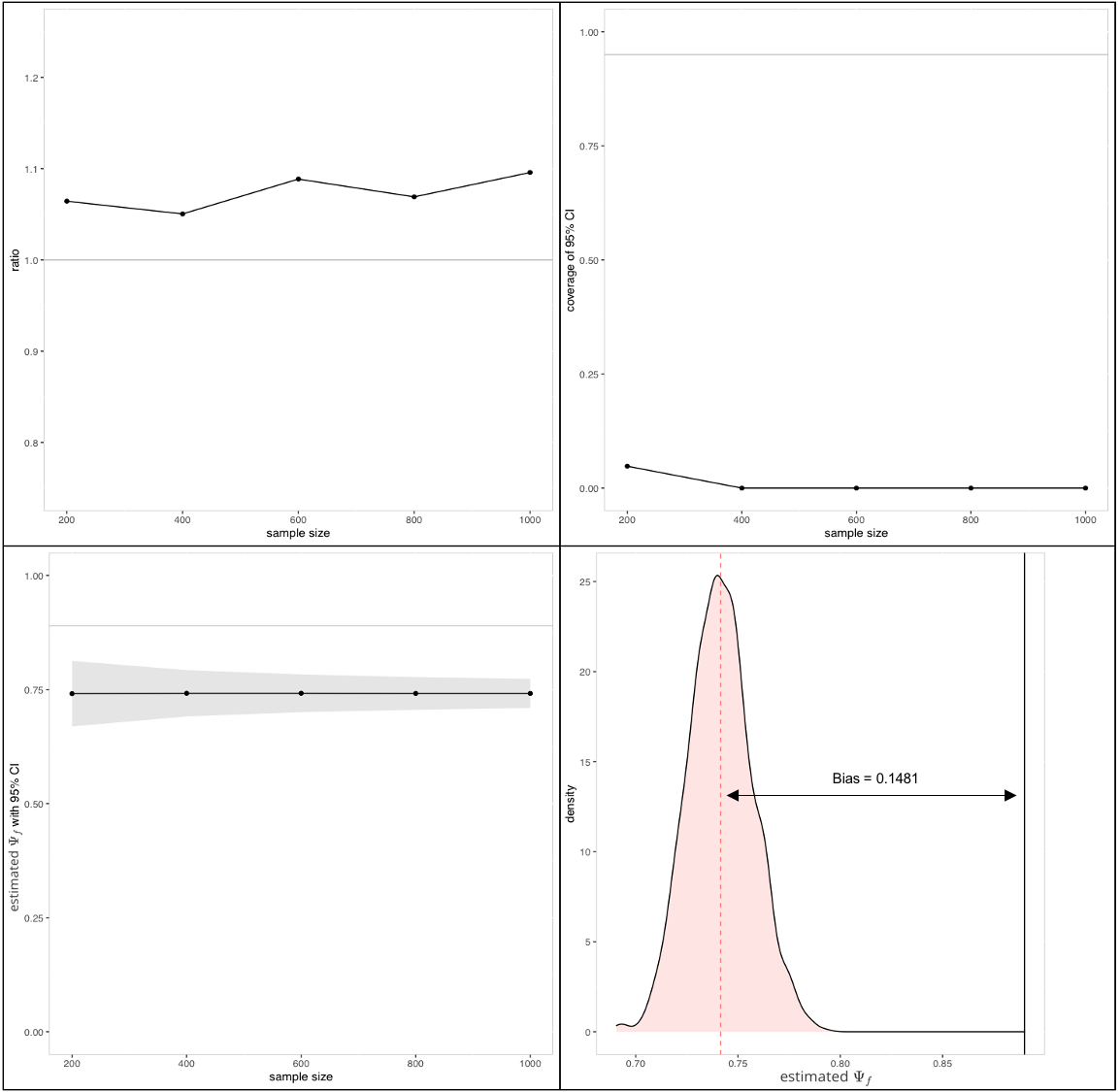
In this section we analyzed the same problem stated in section 5.1, but the identification assumption is violated.
We used the parameters below to generate the underlying distribution. The assumption that the k-way interaction term is violated in this setting().
| 0.11 | 0.1 | 0.05 | 0.08 | -0.2 | -0.2 | -0.1 | 0.2 |
The simulated observed probabilities for all 7 cells are:
| P(0,0,1) | P(0,1,0) | P(0,1,1) | P(1,0,0) | P(1,0,1) | P(1,1,0) | P(1,1,1) |
| 0.2135 | 0.1798 | 0.0449 | 0.2360 | 0.1011 | 0.1978 | 0.0449 |
We can calculate the true value of analytically as , and draw samples to obtain the asymptotic , asymptotic . The asymptotic value is biased by 0.1481.
Figure 7 shows that the linear estimator is biased when the identification assumption is violated.
6.2 Violation of non-linear assumption: independence
Given 3 samples, we suppose that the first and second sample are independent of each other, that is, . Then we can compute and its efficient influence curve as stated above.
Here we illustrate the performance of our estimators with the following underlying distribution:
The probability for all 7 observed cells is given by:
| P(0,0,1) | P(0,1,0) | P(0,1,1) | P(1,0,0) | P(1,0,1) | P(1,1,0) | P(1,1,1) |
| 0.1429 | 0.1429 | 0.1429 | 0.1143 | 0.1143 | 0.1714 | 0.1714 |
We can calculate the true value of analytically as , and draw samples to obtain the asymptotic , asymptotic , the asymptotic value is biased by 0.0794.
Figure 8 shows that violation of the independence assumption will create a significant bias in the results.

6.3 Violation of non-linear assumption: conditional independence
Same as above, our assumption is that given 3 samples, the third sample is independent on the second sample conditional on the first sample . Then we can derive the influence curve same as above.
Here we illustrate the performance of our estimators when the identification assumption does not hold.
The simulated distribution is as follows:
The probability distribution for all 7 observed cells are:
| P(0,0,1) | P(0,1,0) | P(0,1,1) | P(1,0,0) | P(1,0,1) | P(1,1,0) | P(1,1,1) |
| 0.6194 | 0.1749 | 0.0437 | 0.0648 | 0.0648 | 0.0291 | 0.0032 |
The true value of is , and we drew samples and obtained the asymptotic , asymptotic , the asymptotic value is biased by 0.3244.
Figure 9 shows that with a strong violation of conditional independence assumptions, the estimated values will have significant biases.

6.4 Violation of non-linear assumption: K-way interaction term equals zero
Here we illustrate the performance of our estimators when the identification assumption that the k-way interaction term does not hold. We used the parameters below to generate the underlying distribution. The underlying distribution follows the same model as in section 5.3.
| -1.6333 | 0 | 0 | 0 | -1 | -2 | -0.5 | 1 |
The simulated observed probabilities for all 7 observed cells are:
| P(0,0,1) | P(0,1,0) | P(0,1,1) | P(1,0,0) | P(1,0,1) | P(1,1,0) | P(1,1,1) |
| 0.2386 | 0.2386 | 0.0878 | 0.2386 | 0.0323 | 0.1447 | 0.0196 |
Figure 10 and table 7 show that when the assumption is heavily violated, all estimators are significantly biased. The true value of . The bias for estimator is 0.2032, for estimator is 0.1372, for is 0.2055, for estimator is 0.2217, and for estimator is 0.2185. The coverage of 95% asymptotic confidence intervals for estimator is 26%, for estimator is 59%, for is 22%, for and is 0%. Table 8 shows the information on models.

| Estimator | average | lower 95% CI | upper 95% CI | coverage(%) |
|---|---|---|---|---|
| 0.6042 | 0.4491 | 0.7592 | 26.3 | |
| 0.6702 | 0.5261 | 0.8142 | 58.6 | |
| 0.6019 | 0.4516 | 0.7523 | 21.9 | |
| 0.5857 | 0.5416 | 0.6295 | 0 | |
| 0.5889 | 0.5447 | 0.6328 | 0 |
| Estimator | df | AIC | BIC |
|---|---|---|---|
| 5 | 157.720 | 167.535 | |
| 3 | 128.623 | 148.254 |
6.5 Violation of all identification assumptions
In the sections above we showed that if an identification assumption is violated, its corresponding estimators will be biased and their asymptotic confidence intervals will have low coverage. In this section, all the identification assumptions are violated in the simulated distribution, and we analyzed the performance of all the estimators discussed above in this setting.
The underlying distribution of three samples follows the same log-linear model in section 5.3, with the parameters as below.
| -1.1835 | -1 | -1 | -1 | -1.5 | -1 | 2 | 1 |
The simulated observed probability for all 7 observed cells is given by:
| P(0,0,1) | P(0,1,0) | P(0,1,1) | P(1,0,0) | P(1,0,1) | P(1,1,0) | P(1,1,1) |
| 0.1624 | 0.1624 | 0.0133 | 0.1624 | 0.0220 | 0.4414 | 0.0362 |
Figure 11 and table 9 show that all estimators are significantly biased, when none of their identification assumption holds. The true value of . Under the assumption that sample and are independent conditional on (”Conditional Independence” in table 9), the plug-in estimator has a bias of -0.2497. Under the assumption that sample and are independent (”Independence” in table 9), the plug-in estimator has a bias of 0.3760. Under the Under the assumption that the 3-way additive interaction term in the linear model equals zero (”K-way additive interaction equals zero” in table 9), the plug-in estimator has a bias of -0.2627. And under the assumption that the 3-way multiplicative interaction term in the log-linear model equals zero (”K-way multiplicative interaction equals zero” in table 9), the estimator has a bias of 0.2517, the estimator has a bias of -0.1573, the has a bias of -0.1867, the estimator has a bias of -0.1017, and the estimator has a bias of -0.1446. The coverage of 95% asymptotic confidence intervals for all the estimators are far below 95%. Table 10 shows the information on models.

| Assumption | Estimator | Average | Lower 95% CI | Upper 95% CI | Coverage(%) |
|---|---|---|---|---|---|
| Conditional independence | 0.9435 | 0.9313 | 0.9557 | 31.2 | |
| Independence | 0.3223 | 0.2472 | 0.3974 | 0 | |
| Highest-way interaction equals zero (linear) | 0.9565 | 0.8999 | 1.0132 | 0 | |
| Highest-way interaction equals zero (log-linear) | 0.4466 | 0.2519 | 0.6413 | 0 | |
| Highest-way interaction equals zero (log-linear) | 0.8511 | 0.8005 | 0.9017 | 0 | |
| Highest-way interaction equals zero (log-linear) | 0.8805 | 0.8385 | 0.9225 | 31.2 | |
| Highest-way interaction equals zero (log-linear) | 0.7955 | 0.7621 | 0.8269 | 0 | |
| Highest-way interaction equals zero (log-linear) | 0.8384 | 0.8074 | 0.8673 | 0 |
| Estimator | Df | AIC | BIC |
|---|---|---|---|
| 5 | 743.631 | 753.447 | |
| 3 | 391.757 | 411.388 |
7 Data Analysis
Schistosomiasis is an acute and chronic parasitic disease endemic to 78 countries worldwide. Estimates show that at least 229 million people required preventive treatment in 2018 [24]. In China, schistosomiasis is an ongoing public health challenge and the country has set ambitious goals of achieving nationwide transmission interruption [25]. To monitor the transmission of schistosomiasis, China operates three surveillance systems which can be considered as repeated samples of the underlying infected population. The first is a national surveillance system designed to monitor nationwide schistosomiasis prevalence (), which covers 1% of communities in endemic provinces, conducting surveys every 6-9 years. The second is a sentinel system designed to provide longitudinal measures of disease prevalence and intensity in select communities (), and conducts yearly surveys. The third system () comprises routine surveillance of all communities in endemic counties, with surveys conducted on a roughly three-year cycle [25]. In this application, we use case records for schistosomiasis from these three systems for a region in southwestern China [17]. The community, having a population of about 6000, reported a total of 302 cases in 2004: 112 in ; 294 in ; and 167 in ; with 202 cases appearing on more than one system register (figure 12). The three surveillance systems are not independent, and we apply estimators under the four constraints (highest-way interaction equals zero in log-linear model, highest-way interaction equals zero in linear model, independence, and conditional independence)to the data.

The estimated with its 95% asymptotic confidence intervals are shown in table 11. The highest estimate of is 0.9969 (with 95% CI: (0.8041, 0.9829)) under conditional independence assumption, and the lowest is 0.8935 (with 95% CI: (0.9965, 0.9972)) under the linear model with no highest-way interaction assumption (table 11). This analysis illustrates the heavy dependence of estimates of on the arbitrary identification assumptions using real data.
One way to solve this problem is to hold certain identification assumptions true by design. In this case, we could make an effort to design the sentinel system and routine system to be independent of each other conditional on national system . For example, let the sampling surveys in and be done independently, while each of them could borrow information from . In so doing we can assume the conditional independence between the two samples and conduct the analysis correspondingly.
| Assumption | Estimator | Estimated | Lower 95% CI | Upper 95% CI |
|---|---|---|---|---|
| Highest-way interaction equals zero (log-linear) | 0.9212 | 0.8755 | 0.9669 | |
| Highest-way interaction equals zero (log-linear) | 0.9428 | 0.9089 | 0.9768 | |
| Highest-way interaction equals zero (log-linear) | 0.9321 | 0.8959 | 0.9627 | |
| Highest-way interaction equals zero (log-linear) | 0.9934 | 0.9748 | 1 | |
| Highest-way interaction equals zero (linear) | 0.8935 | 0.8041 | 0.9829 | |
| Independence | 0.963 | 0.9326 | 0.9935 | |
| Conditional independence | 0.9969 | 0.9965 | 0.9972 |
| Estimator | Df | AIC | BIC |
|---|---|---|---|
| 5 | 329.383 | 336.804 | |
| 3 | 60.139 | 74.980 |
8 Discussion
8.1 Summary table
In this section we summarise all the estimators we proposed under linear and non-linear constraints as below.
| Identification assumption | Highest-way interaction term in linear model equals zero |
|---|---|
| Constraint | |
| Method | Plug-in |
| Target parameter | |
| Efficient influence curve |
| Identification assumption | Independence between two samples |
|---|---|
| Constraint | |
| Method | Plug-in |
| Target parameter | |
| Efficient influence curve | |
| , | |
| where , | |
| , | |
| Identification assumption | Conditional independence between two samples |
|---|---|
| Constraint | |
| Method | Plug-in |
| Target parameter | |
| Efficient influence curve | , |
| where | |
| Identification assumption | Highest-way interaction term in log-linear model equals zero |
|---|---|
| Constraint | |
| Method | Plug-in (NPMLE), undersmoothed lasso, TMLE based on lasso |
| Target parameter | |
| Efficient influence curve |
We developed a modern method to estimate population size based on capture-recapture designs with a minimal number of constraints or parametric assumptions. We provide the solutions, theoretical support, simulation study and sensitivity analysis for four identification assumptions: independence between two samples, conditional independence between two samples, no highest-way interaction in linear models, and no highest-way interaction in log-linear models. We also developed machine learning algorithms to solve the curse of dimensionality for high dimensional problems under the assumption of no highest-way interaction in log-linear model. Through our analysis, we found that whether the identification assumption holds true plays a vital role in the performance of estimation. When the assumption is violated, all estimators will be biased. This conclusion applies to models of all forms, parametric or non-parametric, simple plug-in estimators or complex machine-learning based estimators. Thus one should always ensure that the chosen identification assumption is known to be true by survey design, otherwise all the estimators will be unreliable. Under the circumstances where the identification assumptions hold true, the performance of our targeted maximum likelihood estimator, , is superior to (identical capture-probabilities, no highest-way interaction in log-linear model), (no interaction terms in log-linear model) and (plugged-in, no highest-way interaction in log-linear model) estimators in several aspects: first, by making the least number of assumptions required for identifiability, the estimator is more robust in empirical data analysis, as there will be no bias due to violations of parametric model assumptions. Second, the estimator is based on a consistent undersmoothed lasso estimator. This property ensures the asymptotic efficiency of TMLE. Third, when there are empty cells, the estimator solves the curse of dimensionality by correcting the bias introduced by the undersmoothed lasso estimator, and gives a more honest asymptotic confidence interval, wider that those from parametric models, and hence a higher coverage.
References
- [1] Anne Chao et al. “The applications of capture-recapture models to epidemiological data” In Statistics in medicine 20.20 Wiley Online Library, 2001, pp. 3123–3157
- [2] Stephen T Buckland et al. “Introduction to distance sampling: estimating abundance of biological populations” Oxford (United Kingdom) Oxford Univ. Press, 2001
- [3] Mathew W Alldredge, Kenneth H Pollock and Theodore R Simons “Estimating detection probabilities from multiple-observer point counts” In The Auk 123.4 Oxford University Press, 2006, pp. 1172–1182
- [4] Anne Chao “An overview of closed capture-recapture models” In Journal of Agricultural, Biological, and Environmental Statistics 6.2 Springer, 2001, pp. 158–175
- [5] Zachary T Kurtz “Local log-linear models for capture-recapture” In arXiv preprint arXiv:1302.0890, 2013
- [6] Janet T Wittes “Applications of a multinomial capture-recapture model to epidemiological data” In Journal of the American Statistical Association 69.345 Taylor & Francis Group, 1974, pp. 93–97
- [7] George Arthur Frederick Seber “The estimation of animal abundance and related parameters” Blackburn press Caldwell, New Jersey, 1982
- [8] Hamparsum Bozdogan “Model selection and Akaike’s information criterion (AIC): The general theory and its analytical extensions” In Psychometrika 52.3 Springer, 1987, pp. 345–370
- [9] Gideon Schwarz “Estimating the dimension of a model” In Annals of statistics 6.2 Institute of Mathematical Statistics, 1978, pp. 461–464
- [10] David Draper “Assessment and propagation of model uncertainty” In Journal of the Royal Statistical Society: Series B (Methodological) 57.1 Wiley Online Library, 1995, pp. 45–70
- [11] Emest B Hook and Ronald R Regal “Validity of methods for model selection, weighting for model uncertainty, and small sample adjustment in capture-recapture estimation” In American journal of epidemiology 145.12 Oxford University Press, 1997, pp. 1138–1144
- [12] Toon Braeye et al. “Capture-recapture estimators in epidemiology with applications to pertussis and pneumococcal invasive disease surveillance” In PloS one 11.8 Public Library of Science San Francisco, CA USA, 2016, pp. e0159832
- [13] Manjari Das and Edward H Kennedy “Doubly robust capture-recapture methods for estimating population size” In arXiv preprint arXiv:2104.14091, 2021
- [14] Mark J Laan and Sherri Rose “Targeted learning: causal inference for observational and experimental data” Springer Science & Business Media, 2011
- [15] Annegret Grimm, Bernd Gruber and Klaus Henle “Reliability of different mark-recapture methods for population size estimation tested against reference population sizes constructed from field data” In PLoS One 9.6 Public Library of Science, 2014, pp. e98840
- [16] Samuel G Rees, Anne E Goodenough, Adam G Hart and Richard Stafford “Testing the effectiveness of capture mark recapture population estimation techniques using a computer simulation with known population size” In Ecological Modelling 222.17 Elsevier, 2011, pp. 3291–3294
- [17] Robert C Spear et al. “Factors influencing the transmission of Schistosoma japonicum in the mountains of Sichuan Province of China” In The American journal of tropical medicine and hygiene 70.1 ASTMH, 2004, pp. 48–56
- [18] Rene Gateaux “Fonctions d’une infinite de variables independantes” In Bulletin de la Societe Mathematique de France 47, 1919, pp. 70–96
- [19] Richard D Gill, Jon A Wellner and Jens Praestgaard “Non-and semi-parametric maximum likelihood estimators and the von mises method (part 1)[with discussion and reply]” In Scandinavian Journal of Statistics JSTOR, 1989, pp. 97–128
- [20] Mark J Laan, David Benkeser and Weixin Cai “Efficient estimation of pathwise differentiable target parameters with the undersmoothed highly adaptive lasso” In arXiv preprint arXiv:1908.05607, 2019
- [21] Richard M Cormack “Log-linear models for capture-recapture” In Biometrics JSTOR, 1989, pp. 395–413
- [22] Sophie Baillargeon and Louis-Paul Rivest “Rcapture: loglinear models for capture-recapture in R” In Journal of Statistical Software 19.5, 2007, pp. 1–31
- [23] Zoe Emily Schnabel “The estimation of the total fish population of a lake” In The American Mathematical Monthly 45.6 Taylor & Francis, 1938, pp. 348–352
- [24] “Schistosomiasis:Key Facts” URL: https://www.who.int/en/news-room/fact-sheets/detail/schistosomiasis
- [25] Song Liang et al. “Surveillance systems for neglected tropical diseases: global lessons from China’s evolving schistosomiasis reporting systems, 1949–2014” In Emerging themes in epidemiology 11.1 Springer, 2014, pp. 19
- [26] Joseph L Doob “The limiting distributions of certain statistics” In The Annals of Mathematical Statistics 6.3 JSTOR, 1935, pp. 160–169
9 Appendix
In the appendix, we formally state the lemmas used in the context and provide the proofs. In section 9.1, we derive the target parameter under identification assumption that the first two samples are independent, given there are three samples in total. In section 9.2 we derive the efficient influence curve for . In section 9.3, we state the lemma on how to derive the efficient influence curve under multidimensional constraint . In section 9.4, we formally state the target parameter under identification assumption that the first two samples are independent conditional on the third samples. In section 9.5 we derive the efficient influence curve for . In section 9.6 we prove the asymptotic efficiency of the TMLE.
9.1 Target parameter under independence assumption
Lemma 1.
For constraint (equation 4), we have the target parameter as:
Proof.
We provide a brief proof of lemma 1 when there are three samples. In this case, is equivalent to
| (17) |
When there are three samples, equation 17 can be expanded as:
| (18) | |||||
Denote , . Equation 18 can be written as:
Plug in , we have
Thus equation 18 can be expressed as:
| (19) |
Here, let , , from equation 19 we know , thus we have
where and ∎
9.2 Efficient influence curve under independence assumption
Lemma 2.
For constraint (equation 4), we have the efficient influence curve as:
| (20) | |||||
Proof.
By the delta method [26], the efficient influence curve of can be written as a function of each components’ influence curve. The efficient influence curves of the three components are presented as follows:
Therefore, we only need to calculate the derivatives to get , and the three parts of derivatives are given by
9.3 Efficient influence curve under multidimensional constraint
Lemma 3.
Consider a model defined by an initial larger model and multivariate constraint function . Suppose that is path-wise differentiable at with efficient influence curve for all . Let be the tangent space at for model , and let be the projection operator onto . The tangent space at for model is given by:
The projection onto is given by:
where is the projection operator on the -dimensional subspace of spanned by the components of . The latter projection is given by the formula:
9.4 Target parameter under conditional independence assumption
Lemma 4.
9.5 Efficient influence curve under conditional independence assumption
Lemma 5.
Proof.
By the delta method [26], the efficient influence curve of can be written as a function of each components’ influence curve. The efficient influence curves of the three components are presented as follows
| (22) | |||||
| (23) | |||||
| (24) | |||||
Therefore, we only need to calculate the derivatives to get , and the three parts of derivatives are given by
where
Plug each part into equation 24, we have that lemma 5 is true. ∎
9.6 Asymptotic efficiency of TMLE
In this section we prove the following theorem 1 establishing asymptotic efficiency of the TMLE. The empirical NPMLE is also efficient since asymptotically all cells are filled up. And TMLE is just a finite sample improvement and asymptotically TMLE acts as the empirical NPMLE. The estimators will be like parametric model MLE and thus converge at rate .
Theorem 1.
Consider the TMLE of defined above, satisfying . We assume for all . If , then is an asymptotically efficient estimator of :
Proof.
Define .Note that
Consider the second order Taylor expansion of at :
where
| (25) | |||||
From equation 25 we know that is a second order term involving square differences for . Thus, we observe that
This proves that
We can apply this identity to so that we obtain . Combining this identity with yields:
We will assume that is consistent for and for all , so that it follows that is uniformly bounded by a with probability tending to 1, an that it falls in a -Donsker class (dimension is finite ), and in probability as . By empirical process theory, it now follows that
We also note that has denominators that are bounded away from zero, so that if (e.g., Euclidean norm). Thus theorem 1 is proved. ∎
10 Acknowledgement
This research was supported by NIH grant R01AI125842 and NIH grant 2R01AI074345.