Estimation of Photometric Redshifts. II. Identification of Out-of-Distribution Data with Neural Networks
Abstract
In this study, we propose a three-stage training approach of neural networks for both photometric redshift estimation of galaxies and detection of out-of-distribution (OOD) objects. Our approach comprises supervised and unsupervised learning, which enables using unlabeled (UL) data for OOD detection in training the networks. Employing the UL data, which is the dataset most similar to the real-world data, ensures a reliable usage of the trained model in practice. We quantitatively assess the model performance of photometric redshift estimation and OOD detection using in-distribution (ID) galaxies and labeled OOD (LOOD) samples such as stars and quasars. Our model successfully produces photometric redshifts matched with spectroscopic redshifts for the ID samples and identifies well the LOOD objects with more than 98% accuracy. Although quantitative assessment with the UL samples is impracticable due to the lack of labels and spectroscopic redshifts, we also find that our model successfully estimates reasonable photometric redshifts for ID-like UL samples and filter OOD-like UL objects. The code for the model implementation is available at https://github.com/GooLee0123/MBRNN_OOD.
1 Introduction
Future astronomical surveys, such as the Legacy Survey of Space and Time (Ivezić et al., 2019), Euclid (Laureijs et al., 2010), and Nancy Grace Roman Space Telescope (Spergel et al., 2013), are expected to explore billions of galaxies whose redshifts should be reliably estimated. The redshifts of galaxies are prerequisites in most extragalactic and cosmological studies (Blake & Bridle, 2005; Bordoloi et al., 2010; Masters et al., 2015). Although spectroscopic measurements yield accurate redshifts of distant galaxies with negligible error (Beck et al., 2016), obtaining spectroscopic redshifts is excessively time-consuming. Moreover, the number of objects to which spectroscopy is applicable is limited because high-quality spectroscopic data are high-priced to acquire particularly for faint objects. The cost of spectroscopic redshifts leads to the use of photometric redshifts as alternatives. Photometric redshifts are less time-intensive and more widely applicable than spectroscopic ones, although their accuracy is generally worse than that of spectroscopic redshifts (Salvato et al., 2019).
Template-based spectral energy distribution (SED) fitting (Bolzonella et al., 2000) and machine-learning inference are two representative approaches for estimating photometric redshifts (Cavuoti et al., 2017). Although the template-based SED fitting provides extensive coverage of redshifts and photometric properties, it can be more computationally expensive than machine-learning inference due to the nature of brute-force search. Besides, the reliance on prior knowledge on SEDs may induce bias in results (Walcher et al., 2011; Tanaka, 2015). Meanwhile, machine-learning approaches enable quick inference of photometric redshifts after training phases (Salvato et al., 2019) as proven in many past studies (Carliles et al., 2010; Gerdes et al., 2010; D’Isanto & Polsterer, 2018; Pasquet-Itam & Pasquet, 2018). Despite this advantage of the machine-learning approaches, the reliability and performance of machine-learning models are guaranteed only when test data follow the distribution of training data in both input and target (i.e., redshift) spaces as in-distribution (ID) data (Goodfellow et al., 2015; Amodei et al., 2016).
It is practically impossible to prepare a training set with complete coverage of the entire input and target (i.e., redshift) spaces extended by the expected real-world data (Domingos, 2012; Yuille & Liu, 2021). The under-represented or unseen galaxies residing outside the property range of training samples for inference of photometric redshifts are drawn from out-of-distribution (OOD) with respect to given machine-learning models (Hendrycks & Gimpel, 2017; Liang et al., 2018; Lee et al., 2018a, b; Ren et al., 2019). The OOD objects in the inference of photometric redshifts can be categorized into two types. One type corresponds to objects such as quasars (QSOs) and stars physically different from galaxies. We call them physically OOD objects. Although the distribution of the physically OOD samples generally deviates from that of ID samples in the input space, some may exist where the ID samples densely populate. For example, the colors of QSOs at some redshifts can be similar to those of galaxies at different redshifts. Hence, the physically OOD samples may be viewed as ID samples from the perspective of the trained model. The second type comprises galaxies unseen or under-represented in training data (hereinafter, under-represented galaxies). The photometric redshifts of under-represented galaxies cannot be successfully inferred by a model due to the nature of inductive reasoning in machine-learning.
In our previous study (Paper I, Lee & Shin (2021)), we focused on the accurate photometric redshift estimation of ID samples that are galaxies well represented by training data, and the trained model successfully inferred photometric redshifts with ID test samples. However, we found that both non-galaxy objects and under-represented galaxies could have an overconfident estimation of photometric redshifts, although the estimation was incorrect. Confidence is a measure of how confident a neural network is about its inference, and it is defined as the maximum value of the probability output for a given sample. Silent failure of trained networks by estimating incorrect photometric redshifts with high confidence for the OOD objects proves that the typical confidence is an unreliable indicator for detecting OODs and may lead to wrong interpretation (Nguyen et al., 2015). Owing to these unreliable results and the vulnerability of trained networks, alternative approaches for OOD detection are required.
In this second paper of a series, we propose a multi-stage-training approach to handle dual tasks: photometric redshift estimation and OOD scoring/detection111We interchangeably use OOD scoring and detection. Specifically, we use the term scoring when emphasizing the sequential property of OOD score and use detection otherwise.. The proposed approach employs unsupervised learning for OOD scoring/detection introduced in Yu & Aizawa (2019) in addition to supervised learning for redshift estimation described in Paper I. Supervised learning requiring labeled samples (i.e., training samples of galaxies with spectroscopic redshifts) in training the model shows a remarkable performance on ID data (Caruana & Niculescu-Mizil, 2006) (see Paper I). We employ unsupervised learning, which trains models with a loss function computable without sample labels (Yamanishi & Takeuchi, 2001; Chui et al., 2004) for using unlabeled (UL) data, presumably containing both ID and OOD data. For inference, we use networks’ outputs from different timelines of the training process to evaluate photometric redshifts and OOD scores. Since the networks trained as such can both detect OOD objects and estimate photometric redshifts, we expect a trained model to perform better with real-world data than a model without handling the OOD samples.
We also expect that our approach employing the UL training data for OOD object detection can achieve a more robust performance regarding the OOD data by handling the more diverse possibility of OOD properties with the UL data than the labeled data. Our trained networks may not be capable of detecting OOD objects populating the regions of the input spaces not covered by the UL data. However, the regions that UL data encompass in the input space can be easily extended because they obviate high costs in labeling training samples.
The rest of the paper is organized as follows. In Section 2, we introduce ID, labeled OOD (LOOD), and UL datasets used for the training and inference of networks. Section 3 describes the proposed multi-stage-training approach for the two tasks: photometric redshift estimation and OOD detection. Section 4 focuses on the performance analysis of the networks for both tasks using ID, LOOD, and UL test datasets. Finally, we summarize our contribution and discuss the future research direction in Section 5.
2 Data
| Dataset name | Number of objects | Selection conditions | Reference |
|---|---|---|---|
| SDSS DR15 | 1294042 | (CLASS GALAXY) and (ZWARNING 0 or 16) and (Z_ERR 0.0) | Aguado et al. (2019) |
| LAMOST DR5 | 116186 | (CLASS GALAXY) and (Z -9000) | Cui et al. (2012) |
| 6dFGS | 45036 | (QUALITY_CODE 4) and (REDSHIFT 1.0) | Jones et al. (2009) |
| PRIMUS | 11012 | (CLASS GALAXY) and (ZQUALITY 4) | Cool et al. (2013) |
| 2dFGRS | 7000 | (Q_Z 4) and (O_Z_EM 1) and (Z 1) | Colless et al. (2001) |
| OzDES | 2159 | (TYPES RadioGalaxy or AGN or QSO or Tertiary) and (FLAG 3 and 6) and (Z 0.0001) | Childress et al. (2017) |
| VIPERS | 1680 | (4 ZFLG 5) or (24 ZFLG 25) | Scodeggio et al. (2018) |
| COSMOS-Z-COSMOS | 985 | ((4 CC 5) or (24 CC 25)) and (REDSHIFT 0.0002) | Lilly et al. (2007, 2009) |
| VVDS | 829 | ZFLAGS 4 or 24 | Le Fèvre et al. (2013) |
| DEEP2 | 540 | (ZBEST 0.001) and (ZERR 0.0) and (ZQUALITY 4) and (CLASS GALAXY) | Newman et al. (2013) |
| COSMOS-DEIMOS | 517 | (REMARKS STAR) and (QF 10) and (Q 1.6) | Hasinger et al. (2018) |
| COMOS-Magellan | 183 | (CLASS nl or a or nla) and (Z_CONF 4) | Trump et al. (2009) |
| C3R2-Keck | 88 | (REDSHIFT 0.001) and (REDSHIFT_QUALITY 4) | Masters et al. (2017, 2019) |
| MUSE-Wide | 3 | No filtering conditions. | Urrutia et al. (2019) |
| UVUDF | 2 | Spectroscopic samples. | Rafelski et al. (2015) |
| Dataset name | Number of objects | Selection conditions | Reference |
|---|---|---|---|
| SDSS DR15 | 290255 | (CLASS QSO) and (ZWARNING 0) and (Z_ERR 0.0) | Aguado et al. (2019) |
| LAMOST DR5 | 32793 | (CLASS QSO) and (Z -9000) | Cui et al. (2012) |
| OzDES | 772 | (TYPES AGN or QSO) and (FLAG 3 and 6) and (Z 0.0025) | Childress et al. (2017) |
| PRIMUS | 155 | (CLASS AGN) and (ZQUALITY 4) | Cool et al. (2013) |
| COMOS-Magellan | 53 | (CLASS bl or bnl or bal) and (Z_CONF 4) | Trump et al. (2009) |
| 6dFGS | 49 | (QUALITY_CODE 6) or (REDSHIFT 1.0) | Jones et al. (2009) |
| COSMOS-DEIMOS | 30 | (QF 10) and (Q 1.6) | Hasinger et al. (2018) |
| VVDS | 16 | ZFLAGS 14 or 214 | Le Fèvre et al. (2013) |
| COSMOS-Z-COSMOS | 5 | (CC 14 or 214) and (REDSHIFT 0.0002) | Lilly et al. (2007, 2009) |
| Dataset name | Number of objects | Selection conditions | Reference |
|---|---|---|---|
| LAMOST DR5 | 4131528 | (CLASS STAR) and (Z -9000) | Cui et al. (2012) |
| SDSS DR15 | 544028 | (CLASS STAR) and (ZWARNING 0) and (Z_ERR 0.0) | Aguado et al. (2019) |
| PRIMUS | 1730 | ZQUALITY -1 | Cool et al. (2013) |
| OzDES | 1138 | FLAG 6 | Childress et al. (2017) |
| COSMOS-DEIMOS | 372 | (REMARKS STAR) and (Q 1.6) | Hasinger et al. (2018) |
| COSMOS-Z-COSMOS | 300 | REDSHIFT 0.0002 | Lilly et al. (2007, 2009) |
| C3R2-Keck | 1 | (REDSHIFT 0.001) and (REDSHIFT_QUALITY 4) | Masters et al. (2017, 2019) |
As described in Paper I, we use the photometric data retrieved from the public data release 1 of the Pan-STARRS1 (PS1) survey as input (Kaiser et al., 2010). The PS1 survey provides photometry in five grizy bands (Chambers et al., 2016). The input data comprise seventeen color-related features: four colors , , , and in PSF measurement, their uncertainties derived using the quadrature rule, the same quantities in Kron measurement, and reddening . We use only valid photometric data, which are found under the condition of ObjectQualityFlags QF_OBJ_GOOD (Flewelling et al., 2020). To make each input feature contribute a similar amount of influence to a model loss function, we rescale input features using min-max normalization in a feature-wise manner.
We use three datasets in training and validating our model: the ID, UL, and LOOD datasets. Each dataset is used for a different purpose. The ID data are galaxy samples used as training data for photometric redshift estimation. We use 1,480,262 galaxies, which are identical to the samples used in Paper I, as summarized in Table 1. The dominant fraction of the training samples comes from the SDSS dataset where about half of them are brighter than 19 magnitude in -band (see Appendix A). We assign 80%, 10%, and 10% of the samples to the training, validation, and test sets (Murphy, 2012) in estimating photometric redshifts for training models, finding the best model, and examining the found model, respectively. Because we randomly split data and have plenty of samples, it is reasonable to assume that the samples allocated to each set follow the same distribution as the ID samples.
The UL data contain UL samples presumably containing both ID and OOD samples, and we do not know their physical classes and spectroscopic redshifts. We use the UL data for the unsupervised training of the model for OOD detection. We construct the entire UL dataset to have 300,055,711 unknown objects following the same selection condition adopted for the ID training samples. From the UL dataset, we evenly draw samples according to right ascension (RA) for unbiased training of the model for OOD detection. We use an RA interval of 10° to divide the UL dataset and randomly choose 1,000,000 samples per RA interval. Hence, 36,000,000 UL samples are drawn from the entire UL dataset. Then, we assign 80%, 10%, and 10% of the samples to the training, validation, and test sets for the purpose of training models, finding optimized models, and investigating the found models as described later, respectively.
The LOOD data comprise physically OOD objects; we define labeled (i.e., spectroscopically classified) QSOs and stars as the LOOD data. We obtain the photometric data of 324,234 QSOs and 4,681,989 stars in the PS1 DR1 following the same selection condition adopted for the ID training samples. The sources of these spectroscopic objects are summarized in Tables 2 and 3. We use the LOOD data for the quantitative assessment of OOD detection performance and exclude them from training the models. Hence, we use the entire LOOD samples as the test data for model validation.
3 Method
To equip the networks with OOD scoring/detection functionality, we train two neural networks and sharing the same structure in a multi-stage-training approach comprising supervised and unsupervised steps (hereinafter, and , respectively) (see Figure 1; Yu & Aizawa (2019)). The two networks are trained differently in to diverge their results on potential OOD samples and evaluate OOD score based on their inference difference. For UL data, one network tries to have a peaked probabilistic distribution of inference on photometric redshifts while the other network intends to generate flat probabilistic distribution as explained later in Section 3.2. The ID data keep the two networks from diverging on ID samples since the training loss using ID samples fosters the two networks to have consistent peaked distributions around the true class, i.e., correct redshift bin.
The training approach consists of three stages: supervised pre-training (training stage-1) with the labeled spectroscopic training samples, iterative supervised and unsupervised training for OOD scoring/detection (training stage-2) with the labeled spectroscopic samples and UL data, respectively, and supervised training for photometric redshift estimation (training stage-3) as the stage-1 conducts. The first two stages of the training procedures are originally proposed in Yu & Aizawa (2019), whereas the third stage is added to improve the model performance for the original task, i.e., photometric redshift estimation, with the added networks for the OOD detection.
We adopt the same supervised learning technique as Paper I in estimating photometric redshifts as and the unsupervised method using two networks introduced by Yu & Aizawa (2019) in OOD detection as . In the following subsections, we outline , , the three-stage training procedure, and assessment metrics to measure model performance. For a more detailed explanation of each training step, refer to Paper I and Yu & Aizawa (2019).
3.1 Supervised Training Step for Photometric Redshift Estimation
In using only ID data, we bin redshift ranges and classify samples into the redshift bins instead of conducting typical regression of redshifts as we name the model the multiple-bin regression with the neural network used in Paper I. We adopt 64 independent bins with a constant width following the performance result in Paper I. Then, the model estimates probabilities that the photometric redshifts of input samples lie in each bin. Using the model output probabilities, we may obtain point-estimation of photometric redshift by averaging the central redshift values of the bins with the output probabilities.
As a training loss of , we use anchor loss . The loss is designed to measure the difference between two given probability distributions considering prediction difficulties due to various reasons, e.g., the lack of data or the similarities among samples belonging to different classes, i.e., redshift bins. The anchor loss assigns the difficult samples for prediction high weights governed by a weighting parameter . For an in-depth definition of the loss, refer to Ryou et al. (2019). Since we train two networks with the same architecture for the dual tasks, the training loss of , which should be minimized, is set as follow:
| (1) |
where and are the model output probability distributions coming from and , respectively, is a redshift bin vector, and is an ID input vector.
3.2 Unsupervised Training Step for Out-of-Distribution Detection
uses the UL data, presumably containing both ID and OOD samples, in training models and employs the disparity of the results from two networks to evaluate the OOD score of the samples. The two networks are trained to maximize disagreement between them in the photometric redshift estimation for the potential OOD samples, pushing the OOD samples outside the manifold of the ID samples. The two networks, which are identically structured and trained on the same ID data via supervised learning, might have different results on OOD samples because of stochastic effects, although the networks are not optimized for OOD detection. Then, by defining discrepancy loss to measure the disagreement and maximizing it, the two networks can be forced to produce divergent results for the potential OOD samples, which generally correspond to the samples in the class (i.e., redshift bin) boundaries and/or are misclassified (i.e., assigned to an incorrect redshift bin). The defined for this purpose is as follows:
| (2) |
where is the entropy for given probability distributions. As the networks are trained to maximize the discrepancy , the entropies from and output increase and decrease, respectively. The network outputs a flat probability distribution (i.e., high entropy; high uncertainty), and the network generates a peaked one (i.e., low entropy; low uncertainty). Notably, the is available in the unsupervised approach using the UL samples since it can be computed without sample labels (i.e., redshifts). The potential ID samples make it difficult for the two networks produce discrepant inference results for photometric redshifts since the inference for the ID samples has a strongly peaked distribution in both networks and as explained below. Meanwhile, the potentially OOD samples can increase as the two networks become easily divergent in the training process.
To prevent divergent results on the ID samples, we employ the sum of and as the training loss of . Although the unsupervised approach using the diverge the model outputs on the probable OOD examples included in the UL dataset, it can also cause discrepant results on the ID samples since the UL data includes ID and OOD samples. Hence, defining the training loss of as the sum help the two network outputs on the ID samples stay as similar as possible since minimizing encourages the network outputs unimodal probability distributions with a peak at the true class on ID samples. Namely, diverges model outputs for OOD samples more than ID ones because OOD samples are out of support of the . The training loss of , which should be minimized in training, is defined as follows:
| (3) |
where is an UL input vector and is a margin. Notably, is maximized as is minimized due to the negative sign. The use of the margin is required to prevent overfitting of the networks by replacing the second term of the unsupervised loss with zero if . We use found as the best parameter in multiple trial runs.
Our usage of as the combination of and can be understood as multi-task learning of both estimating photometric redshifts and evaluating OOD scores. Particularly, this multi-task learning model is a case of transferring the knowledge of supervised learning (i.e., the model with in estimating photometric redshifts) to unsupervised learning (i.e., the model with in evaluating OOD scores) (Pentina & Lampert, 2017). The combined loss in our dual-task learning adopts the parameter , which regularizes the contribution of to the total loss . This is a simple strategy to find balance among multiple tasks as commonly used as weight parameters with multiple losses in multi-task learning (Sener & Koltun, 2018; Gong et al., 2019; Vandenhende et al., 2021).
3.3 Three-Stage Training

We proceed with the three-stage training of the two networks. Each training stage comprises aforementioned and as summarized in Figure 1. Training stage-1 is a pre-training of the two networks with the . The purpose of this stage is to obtain a stable performance of the networks in estimating photometric redshifts. In training stage-2, the two networks are trained for OOD detection using an iterative training procedure comprising one and two s. Although included in helps the disparity between two network outputs on ID samples stay small, the disparity increases as the models are trained by the optimization using UL samples and . Composing the stage-2 as the iterative training procedure incorporating further precludes the disparity on the ID samples from increasing as included in affects the total loss (see Equation 3). Therefore, as the training continues, the disagreement of the network outcomes for the probable OOD samples becomes larger than that for the ID samples because the OOD samples are outside the support of the , which is only applied to the ID galaxies. Then, the measure of disagreement (i.e., ) can be used as an OOD score to flag OOD candidates. At the inference level, the trained networks in training stage-2 are used to score the test samples as OOD.
In addition to training stage-1 and -2, we proceed to an additional supervised training stage, training stage-3, with for photometric redshift estimation. The unsupervised training for OOD detection affects the model performance of the original task (i.e., photometric redshift estimation) because the model in training stage-2 is optimized for two losses described in Equation 3. In practice, training stage-3 might not be needed if the models trained in stage-1 are saved and used for the task of photometric redshift estimation. In this work, we train the two networks again using only after training stage-2. Then, the outputs of the two stage-3 networks are combined by averaging them to estimate photometric redshifts.
3.4 Assessment Metrics
Since our model performs the two tasks together, we need separate metrics to assess model performances on both tasks. As point-estimation metrics in estimating photometric redshifts with photometric redshifts as mean value with probabilistic inference by the trained model, we adopt the ones used in Paper I: bias, MAD, , , NMAD, and . For a detailed explanation of the metrics, refer to Paper I. In short, the bias is measured as the absolute mean of which is difference between photometric redshifts and true spectroscopic redshifts. Similarly, the MAD is the mean of the absolute difference . and corresponds to the standard deviation of and the 68th percentile of , respectively. NMAD is defined to be 1.4826 median of . presents the fraction of data with . Notably, the lower the point-estimation metrics are, the higher the performance is.
Before explaining OOD detection metrics, we first define four measures: true negative (TN), true positive (TP), false negative (FN), and false positive (FP). The Boolean values (i.e., true and false) in the terms indicate whether the predicted class of the sample is correct or incorrect. The negative and positive in the terms mean the true class in which the given sample is included. We, respectively, set ID and OOD as negative and positive since the model performs OOD detection as a task. Hence, for example, the number of true positive cases is the number of correctly classified OOD samples. The numbers of these four cases can be varied with respect to the adopted threshold of the OOD score. Notably, these metrics are used with the LOOD samples not in training the model but in validating the trained model.
We use the central value between the minimum and maximum as the threshold to compute the metrics. Note that this threshold is chosen simply because it can be easily estimated for model assessment. The following is a brief explanation of the detection metrics.
-
•
Accuracy: ratio of the correctly classified samples to the entire samples ,
-
•
Precision: ratio of the correctly classified positive samples to the entire positively classified samples ,
-
•
True Positive Rate (TPR) or recall: fraction between the correctly predicted positive samples and the entire positive samples ,
-
•
: harmonic mean of precision and recall weighted by . The lesser and larger gives more weight to precision and recall, respectively. Typical values for is 0.5, 1.0, and 1.5. In this work, we set () to focus on more recall than precision, paying attention to the number of the correctly classified OOD samples among all OOD samples,
-
•
: area under the receiver operating characteristic (ROC) curve. The ROC curve is a visualized measure of the detection performance for the binary classifier. In the curve, the TPR is plotted as a function of the false positive rate for different thresholds of the OOD score. False Positive Rate is a fraction between the incorrectly predicted negative samples and entire negative samples . The offers a comprehensive measure of the detection performance of the model.
-
•
: area under the precision-recall (PR) curve. Although offers a representative measure of binary detection performance generally, it may produce misleading results for imbalanced data because TPR (i.e., the vertical axis of the ROC curve) depends only on positive cases without considering negative cases. In the PR curve, precision is plotted as a function of recall. Because precision considers both positive and negative samples, may be more informative for imbalanced data.
The higher values of the detection metrics indicate better detection performance of the model. Notably, these OOD detection metrics are evaluated with the labeled ID (i.e., galaxies) and OOD (i.e., stars and QSOs confirmed spectroscopically).
4 Results
We present the results of the model in testing the two tasks. All results in this section are produced with the samples in the test dataset unless otherwise stated.
4.1 Photometric Redshift Estimation on In-Distribution Samples
| Variables | metrics | |||||
|---|---|---|---|---|---|---|
| Case | Bias | MAR | NMAD | |||
| Stage-2 (high entropy) | 0.0306 | 0.0466 | 0.0959 | 0.0343 | 0.0314 | 0.0637 |
| Stage-2 (low entropy) | 0.0015 | 0.0281 | 0.0444 | 0.0293 | 0.0280 | 0.0150 |
| Stage-3 (average) | 0.0020 | 0.0254 | 0.0392 | 0.0272 | 0.0256 | 0.0087 |


We find that the networks in training stage-3 outperform the networks in the stage-2 in terms of photometric redshift estimation. To verify the effectiveness of the additional stage training stage-3, we compare the quality of the photometric redshifts derived from the models in training stage-2 and -3. Table 4 shows the point-estimation metrics evaluated in the high and low entropy models (high and low entropy models, i.e., and , respectively) in training stage-2 and the averaged model in stage-3. Except for the bias, the training stage-3 model outperforms others. It proves that unsupervised training of the networks in training stage-2 for OOD detection affects the quality of photometric redshifts as expected for multi-task learning.
The networks in training stage-2 hold noticeable peculiarities showing deteriorated photometric redshifts. As shown in Figure 2, the photometric redshifts from the high entropy model are overestimated for a large fraction of samples. Meanwhile, the photometric redshifts from the low entropy model show concentrations at and . The peculiarities in the derived photometric redshifts arise from the minimization of during training stage-2, which makes the output probability distributions of the high and low entropy models flat and peaked, respectively. These oddities of the training stage-2 model vanish in the averaged stage-3 model (see Figure 3). The Pearson correlation coefficient affirms that the estimated photometric redshifts match spectroscopic redshifts well.
4.2 Out-of-Distribution Score for Labeled Data
| Step | Accuracy | Precision | Recall | |||
|---|---|---|---|---|---|---|
| Stage-2 | 0.9802 | 0.9987 | 0.9808 | 0.9863 | 0.9938 | 0.9998 |
| Stage-3 | 0.0295 | 0.9990 | 0.0008 | 0.0012 | 0.7547 | 0.9914 |


As we design and expect, training stage-2 model shows better separation between the ID and OOD samples (i.e., physically OOD samples of stars and QSOs) than the stage-3 model. We compare the OOD detection performance of the networks in training stage-2 and -3. The detection metrics of the networks in training stage-2 and -3 are tabulated in Table 5, showing that the OOD detection model is optimized in training stage-2.
Interestingly, the training stage-3 model has higher precision than the stage-2 model, which is due to the high TP values with the small number of samples flagged as OOD by the training stage-3 model; 352,055 samples () among 5,006,223 true OODs are correctly classified as OOD. This small number results in unexpectedly high precision, , and for the training stage-3 model.
The stage-2 model separates well the labeled ID and OOD samples as shown in Figure 4 displaying the distributions of the ID, LOOD, and UL samples in training stage-2. Although most ID samples appear in low ranges, most LOOD samples are distributed in the vicinity of the highest . In addition, most UL samples show high values. There are small portions of the UL and LOOD samples with the low , which represents samples with the input properties similar to those of the ID samples. We infer that the highest proportion of UL samples are more likely to be OOD objects (including physically OOD objects such as stars and QSOs) than ID galaxies although we cannot specify the classes of the samples. The distribution of the in the UL samples makes sense because the largest fraction of sources should be stars in our Galaxy.
The prediction difficulties of photometric redshift estimation and OOD scores for the ID data are related as presented in Figure 5. Although most samples with non-catastrophic (hereinafter, non-cat) estimation (i.e., ) are assigned to the low group, most samples with catastrophic (hereinafter, cat) estimation of photometric redshifts belong to middle or high groups. High samples generally more deviate from the slope-one line than low samples, indicating that the samples with high OOD score can be viewed as OOD-like ID samples and tend to have incorrect photometric redshifts.
The distributions of for the ID non-cat and cat samples shown in Figure 6 also affirm our interpretation of the relation between and the error in photometric redshifts. The distributions show that a higher fraction of cat samples populates in the high ranges than non-cat samples. Although the number of non-cat samples decreases as the increases, the cat samples are almost uniformly distributed over the entire range. The difficulties in estimating photometric redshifts are related to the OOD-like ID samples222In Paper I, we have already found that the lack of training samples causes high errors in photometric redshifts..
The training stage-3 model is unreliable concerning cat samples with high . As shown in Figure 6, the number of non-cat samples with high confidence on photometric redshifts decreases as increases. The cat samples mostly have low confidence on photometric redshifts throughout low and middle ranges. It also shows that the networks in the training stage-3 are well calibrated in estimating photometric redshifts for the cat samples with low and middle presenting the low confidence on them. However, the cat samples with high extend to cases with high confidence which is the indication of overconfident results on the wrong photometric redshift estimation for OOD-like ID cat samples. It also emphasizes the importance of the OOD detection algorithm since we cannot filter the OOD samples simply based on confidence on photometric redshifts without the OOD score.
The distribution of in the space of input features allows us to visually inspect the OOD-like ID samples. In Figure 7333 This visual presentation often used hereafter displays the projected dimensions of the input space with degeneracy of the input features in the higher dimension., most high samples reside in the low-density regions of the training samples. The training stage-2 model is optimized to assign high OOD scores to under-represented galaxies, meaning that these high ID samples are under-represented galaxies from the model perspective.
As we find the ID samples with high , there are LOOD samples with low (i.e., the ID-like LOOD samples). As presented in Figure 8 depicting the distributions for the two types of LOOD objects, i.e., QSOs and stars, a fraction of LOOD samples have low although most samples have high . The points to be noted are as follows: 1) both QSO and star distributions have peaks at the lowest bin, 2) the ratio of the lowest peak to the highest peak for QSO is larger than that of star, and 3) more QSOs are distributed in the low and middle ranges than stars.
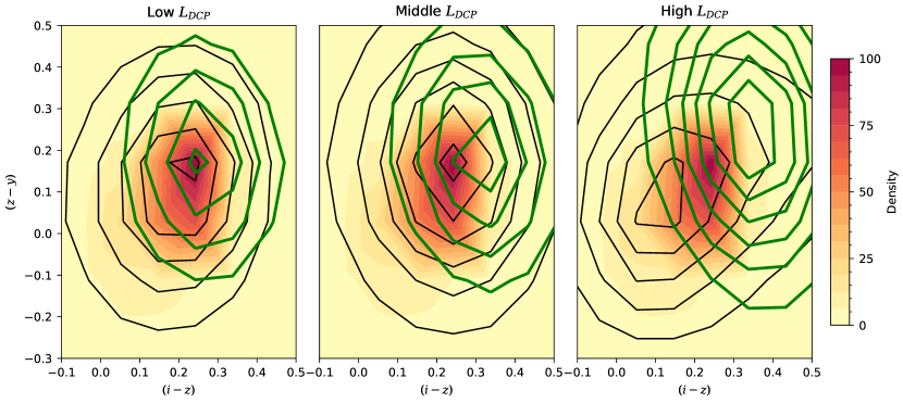
The ID-like LOOD samples locate around the ID sample distribution in the input space. Figure 9 shows that the QSO samples with high overwhelm the ones with low outside the ID sample density contours. However, the number of the low samples for QSOs increases as they approach the ID sample density peak. These ID-like QSOs contribute to the peak at the lowest bin of Figure 8.
As found in Figure 9, some stars certainly reside inside the contours of the ID galaxy samples with respect to the projected input dimension, corresponding to the stars with low (Figure 8). However, most stars have input features significantly deviating from the typical properties of the ID galaxy samples in any one dimension of the input features. Compared with the QSO distribution shown in Figure 9, more stars than QSOs can be sorted out from the ID samples in higher dimensions of input features since the star distribution significantly differs from that of the ID samples. Therefore, the relatively smaller peak of stars at the lowest OOD score and a lower fraction of ID-like stars than QSOs arise as shown in Figure 8.
Filtering out the QSO and star samples with low/middle enables further reliable usage of the trained model for photometric redshifts. As depicted in Figure 10, although the confidence of ID samples gradually reduces as increases, the LOOD objects with high have higher confidence than those with low . Using this distribution difference in the space of and confidence, a considerable number of LOOD samples with low and middle can be filtered by checking their higher confidence than that of ID samples.
4.3 Out-of-Distribution Score and Photometric Redshifts of Unlabeled Data


Because the UL data have no labels and spectroscopic redshifts, we assess the model performance on the UL samples indirectly. To measure the performance of detecting the physically OOD samples in the UL dataset, we first extract the point-source score (hereinafter, ps-score) from Tachibana & Miller (2018) for the UL samples. The ps-score is a machine-learning-based probabilistic inference on being point sources for PS1 objects with the range of [0, 1]. The samples with low ps-score are more likely to be extended sources, i.e., mainly galaxies, and we expect our OOD detection algorithm to produce low for samples with low ps-score.
The distributions of with respect to ps-score are subject to the expected pattern. Figure 11 shows the distribution of the samples under-sampled from the UL dataset within the RA ranges [0, 10], [100, 110], and [170, 180]. The samples within the lowest ps-score interval are mostly distributed near the minimum and maximum values, and the distributions of the higher ps-score samples shift toward high ranges. We conjecture that the middle/high samples with low ps-score are highly likely to be under-represented galaxies residing in the outskirts or low-density parts of the ID distribution (see discussion for Appendix A). Except for this understandable difference, the two machine-learning models reach a consensus on other UL samples which are mainly point-source stars and QSOs.
Figure 12 indirectly proves to be a reliable OOD score for a broad range of input space for the UL samples. The UL samples with low have the most similar distributions to those of the ID samples because the networks assign low to the UL samples with input features comparable with the ID samples. The UL samples with middle begins to display discrepancies from the ID samples in input features distributions. The samples in the high group have a completely different distribution from the ID samples. In the increasing order of the OOD score (i.e., ), the UL data density distributions in the input color spaces deviate more from those of ID samples. As expected from the typical colors of stars (e.g., Jin et al., 2019), the peak in the color distribution for the high- UL samples in Figure 12 corresponds to common stellar colors.
The training stage-3 model adequately produces photometric redshifts for the UL samples. As examined with the ID and LOOD samples, we expect the photometric redshift distributions to be similar to those of ID samples for the UL samples with low and random guessing, i.e., uniform distribution, for the UL samples with high , respectively. As presented in Figure 13, the samples in the low range mostly reside inside the ID sample density contours. On the other hand, the photometric redshifts of the OOD-like samples randomly spread in the spaces without any strong systematic patterns. It certainly shows that the photometric redshift distribution for OOD-like samples are closer to a uniform distribution than ID-like samples. However, most redshifts are in the region . It arises from the fact that approximately % of the training samples for photometric redshifts are found in the region .
We examine the UL samples with the low ps-score and their in the input feature space. These samples generally correspond to galaxies not well represented by the training data. Naturally, the UL samples include more faint galaxies than the spectroscopic training samples because the procedure of selecting spectroscopic targets is generally biased to bright samples. Furthermore, the color and photometric-redshift distributions of the UL samples with the low ps-score and high affirms that these UL samples have input features that are not well represented by the training samples (see Figure 14).
5 Discussion and Conclusion
In this study, we propose a new approach not only to estimate photometric redshifts but also to check the reliability of such redshifts through OOD scoring/detection. The proposed model successfully estimates the photometric redshifts of galaxies using our previous model (presented in Paper I), even with an additional network to detect the OOD samples. Our trained model is available with the Python code, which is based on PyTorch (Paszke et al., 2019), on GitHub444https://github.com/GooLee0123/MBRNN_OOD under an MIT License (Lee & Shin, 2021) for public usage.
The proposed method to detect the OOD data with the photometric redshift inference model shows that the new model can measure how much OOD data deviate from the training data. Most samples with a catastrophic redshift estimation correspond to data with high OOD scores (see Figure 5). However, our model estimating the OOD score cannot replace models that separate galaxies from stars and QSOs. As shown in Figure 10, numerous stars and QSOs exhibit low OOD scores and high confidence values for photometric redshifts in our model although they are physically OOD objects. These objects have indistinguishable input features compared with galaxies in terms of the features used for photometric redshift estimation.
We plan to apply the SED-fitting methods to galaxies with high OOD scores or low confidence values. The machine-learning inference model has limitations that depend on the training samples. Therefore, combining the SED-fitting methods with machine-learning inference models can be an effective strategy to achieve high analysis speed and accuracy. This would have broad applicability in estimating photometric redshifts for numerous galaxies expected for future surveys such as the Legacy Survey of Space and Time (Ivezić et al., 2019).
The current implementation using two networks needs to be improved to see the full benefits of ensemble learning. The multiple anchor loss parameters presented in Paper I are required for more precise estimation of photometric redshifts and evaluation of the OOD scores in a single machine-learning framework. The proposed model in this Paper II excludes multiple inferences of photometric redshifts in ensemble learning. The ensemble model distillation might be a possible technique to accommodate the multiple models included in the ensemble learning as a single combined model (e.g., Malinin et al., 2020) in the current framework combining inference of both photometric redshifts and OOD score. We plan to develop the implementation of the ensemble distillation in the future.
Identifying the influential data among the under-represented galaxies in the UL data can play a key role in improving the quality of photometric redshifts. Including influential data in training can alter the machine-learning model significantly, thereby reducing the fraction of incorrect estimation and/or the uncertainty of estimation (Charpiat et al., 2019; Pruthi et al., 2020). Because the influence of data relies on the model, the future method needs to have a model-dependent algorithm to assess the influence of such data quantitatively. The highly influential data among the OOD samples requires labeling, i.e., acquiring spectroscopic redshifts, to be used as learning samples (Masters et al., 2015; Newman et al., 2015).
Understanding the nature of the under-represented galaxies will be also crucial in improving the evaluation of the OOD score and finding useful samples that need spectroscopic labeling. A large fraction of OOD samples might be produced by effects such as source blending (including physically merging galaxies) and bias in the spectroscopic target selection. When selecting highly influential OOD samples among the UL data, our new algorithm for the OOD score may need a step of filtering out the photometrically unreliable samples such as blended galaxies. The under-represented galaxies might include galaxies with less common physical properties; e.g., extreme dust obstruction, unusual stellar populations, short post-starburst phase, unusually intensively star-forming galaxies, merging galaxies at various evolutionary stages, and galaxies with weak QSO emission.
Semi-supervised learning methods might be an alternative approach to the supervised learning such as our proposed approach. Although semi-supervised learning has its own limitations such as smoothness assumption (Chapelle et al., 2006), semi-supervised learning models intrinsically do not have the OOD problem, except for physically OOD samples. However, the efficacy and reliability of the semi-supervised learning is a new challenge compared with supervised learning methods. Measuring the influence of data on the training and implementation of the algorithm is crucial because the performance of semi-supervised learning methods is strongly subjective to the labeled samples and the weights of UL samples.
Appendix A Example of under-represented galaxies in training data and
We demonstrate a typical case of selection effects based on brightness in spectroscopic training data as an example of considering OOD data. Since the brightness of objects is a main factor affecting target selection in spectroscopy, we examine an extreme case when training samples of spectroscopic redshifts consist of only bright objects, and data for inference include only faint objects. This case undoubtedly demonstrates our model to detect OOD data works well.
Adopting the neural network model in the same way as described in Section 3, we train the model with the bright SDSS spectroscopic objects, which have -band Kron magnitude less than or equal to 19, as supervised training samples. The properties of the 634,928 bright SDSS objects are different from those of the 659,114 faint objects as expected in the SDSS data (see Figure A.1). The bright objects generally have lower redshifts and bluer color than the faint objects have. Therefore, a large fraction of the faint objects should be OOD objects with respect to the trained model as under-represented galaxies in the training data.


The performance in estimating photometric redshifts is much worse for the faint objects than for the bright test samples. As shown in Figure A.2, the trained model cannot estimate correct photometric redshifts for the majority of the faint objects because they are under-represented objects, i.e., OOD objects. The point-estimation metrics also show that the model is not able to infer photometric redshifts for the faint objects. For example, values are 0.0012 and 0.22 for the bright test samples and the faint objects, respectively. The bias value for the bright test samples is about 0.004 while that value for the faint objects is about 0.09.
Our method to evaluate works well in this demonstration. Figure A.3 shows that our method successfully gives the faint objects high . The training data composed of the bright objects do not cover a substantial range of redshifts and input features for the faint test objects as presented in Figure A.1. Most of the faint objects have high as we expect. Because most UL samples are stars in our Galaxy or faint objects, they also show high values in Figure A.3.
Colors as well as their high uncertainties of the faint SDSS objects, which have the high values, display distinct deviation from those of the bright spectroscopic samples (see Figure A.4). Because we use -band magnitude to divide the SDSS spectroscopic samples into the bright and faint sets, redder objects are more likely to be OOD objects as faint objects. As presented in Figure A.4, the faint spectroscopic galaxies showing high have significantly redder and colors than the training samples used to derive the model.
The colors of the UL samples with high are clearly different from those of the faint galaxies with high . In Figure A.4, the peak of the color distribution for the UL samples with high is much bluer than those of both the bright and faint SDSS galaxies with high . Considering the typical distribution of colors for stars, QSOs, and galaxies in the SDSS filter bands (e.g. Finlator et al., 2000; Hansson et al., 2012; Jin et al., 2019), the peak in the color distribution for the UL samples corresponds to the expected colors of stars and low-redshift QSOs.
References
- Aguado et al. (2019) Aguado, D. S., Ahumada, R., Almeida, A., et al. 2019, ApJS, 240, 23, doi: 10.3847/1538-4365/aaf651
- Amodei et al. (2016) Amodei, D., Olah, C., Steinhardt, J., et al. 2016, Concrete Problems in AI Safety. https://arxiv.org/abs/1606.06565
- Beck et al. (2016) Beck, R., Dobos, L., Budavári, T., Szalay, A. S., & Csabai, I. 2016, MNRAS, 460, 1371, doi: 10.1093/mnras/stw1009
- Blake & Bridle (2005) Blake, C., & Bridle, S. 2005, Monthly Notices of the Royal Astronomical Society, 363, 1329, doi: 10.1111/j.1365-2966.2005.09526.x
- Bolzonella et al. (2000) Bolzonella, M., Miralles, J. M., & Pelló, R. 2000, A&A, 363, 476
- Bordoloi et al. (2010) Bordoloi, R., Lilly, S. J., & Amara, A. 2010, Monthly Notices of the Royal Astronomical Society, 406, 881, doi: 10.1111/j.1365-2966.2010.16765.x
- Carliles et al. (2010) Carliles, S., Budavári, T., Heinis, S., Priebe, C., & Szalay, A. S. 2010, The Astrophysical Journal, 712, 511, doi: 10.1088/0004-637x/712/1/511
- Caruana & Niculescu-Mizil (2006) Caruana, R., & Niculescu-Mizil, A. 2006, in Proceedings of the 23rd International Conference on Machine Learning, ICML ’06 (New York, NY, USA: Association for Computing Machinery), 161–168, doi: 10.1145/1143844.1143865
- Cavuoti et al. (2017) Cavuoti, S., Amaro, V., Brescia, M., et al. 2017, MNRAS, 465, 1959, doi: 10.1093/mnras/stw2930
- Chambers et al. (2016) Chambers, K. C., Magnier, E. A., Metcalfe, N., et al. 2016, arXiv e-prints, arXiv:1612.05560. https://arxiv.org/abs/1612.05560
- Chapelle et al. (2006) Chapelle, O., Schölkopf, B., & Zien, A. 2006, Semi-Supervised Learning (Adaptive Computation and Machine Learning) (The MIT Press)
- Charpiat et al. (2019) Charpiat, G., Girard, N., Felardos, L., & Tarabalka, Y. 2019, in Advances in Neural Information Processing Systems 32: Annual Conference on Neural Information Processing Systems 2019, NeurIPS 2019, December 8-14, 2019, Vancouver, BC, Canada, ed. H. M. Wallach, H. Larochelle, A. Beygelzimer, F. d’Alché-Buc, E. B. Fox, & R. Garnett, 5343–5352. https://proceedings.neurips.cc/paper/2019/hash/c61f571dbd2fb949d3fe5ae1608dd48b-Abstract.html
- Childress et al. (2017) Childress, M. J., Lidman, C., Davis, T. M., et al. 2017, MNRAS, 472, 273, doi: 10.1093/mnras/stx1872
- Chui et al. (2004) Chui, H., Rangarajan, A., Zhang, J., & Leonard, C. 2004, IEEE Transactions on Pattern Analysis and Machine Intelligence, 26, 160, doi: 10.1109/TPAMI.2004.1262178
- Colless et al. (2001) Colless, M., Dalton, G., Maddox, S., et al. 2001, MNRAS, 328, 1039, doi: 10.1046/j.1365-8711.2001.04902.x
- Cool et al. (2013) Cool, R. J., Moustakas, J., Blanton, M. R., et al. 2013, ApJ, 767, 118, doi: 10.1088/0004-637X/767/2/118
- Cui et al. (2012) Cui, X.-Q., Zhao, Y.-H., Chu, Y.-Q., et al. 2012, Research in Astronomy and Astrophysics, 12, 1197, doi: 10.1088/1674-4527/12/9/003
- D’Isanto & Polsterer (2018) D’Isanto, A., & Polsterer, K. L. 2018, A&A, 609, A111, doi: 10.1051/0004-6361/201731326
- Domingos (2012) Domingos, P. 2012, Communications of the ACM, 55, 78, doi: 10.1145/2347736.2347755
- Finlator et al. (2000) Finlator, K., Ivezić, Ž., Fan, X., et al. 2000, AJ, 120, 2615, doi: 10.1086/316824
- Flewelling et al. (2020) Flewelling, H. A., Magnier, E. A., Chambers, K. C., et al. 2020, ApJS, 251, 7, doi: 10.3847/1538-4365/abb82d
- Gerdes et al. (2010) Gerdes, D. W., Sypniewski, A. J., McKay, T. A., et al. 2010, The Astrophysical Journal, 715, 823, doi: 10.1088/0004-637x/715/2/823
- Gong et al. (2019) Gong, T., Lee, T., Stephenson, C., et al. 2019, IEEE Access, 7, 141627, doi: 10.1109/ACCESS.2019.2943604
- Goodfellow et al. (2015) Goodfellow, I. J., Shlens, J., & Szegedy, C. 2015, in 3rd International Conference on Learning Representations, ICLR 2015, San Diego, CA, USA, May 7-9, 2015, Conference Track Proceedings, ed. Y. Bengio & Y. LeCun. http://arxiv.org/abs/1412.6572
- Hansson et al. (2012) Hansson, K. S. A., Lisker, T., & Grebel, E. K. 2012, MNRAS, 427, 2376, doi: 10.1111/j.1365-2966.2012.21659.x
- Hasinger et al. (2018) Hasinger, G., Capak, P., Salvato, M., et al. 2018, ApJ, 858, 77, doi: 10.3847/1538-4357/aabacf
- Hendrycks & Gimpel (2017) Hendrycks, D., & Gimpel, K. 2017, in 5th International Conference on Learning Representations, ICLR 2017, Toulon, France, April 24-26, 2017, Conference Track Proceedings (OpenReview.net). https://openreview.net/forum?id=Hkg4TI9xl
- Ivezić et al. (2019) Ivezić, Ž., Kahn, S. M., Tyson, J. A., et al. 2019, ApJ, 873, 111, doi: 10.3847/1538-4357/ab042c
- Jin et al. (2019) Jin, X., Zhang, Y., Zhang, J., et al. 2019, MNRAS, 485, 4539, doi: 10.1093/mnras/stz680
- Jones et al. (2009) Jones, D. H., Read, M. A., Saunders, W., et al. 2009, MNRAS, 399, 683, doi: 10.1111/j.1365-2966.2009.15338.x
- Kaiser et al. (2010) Kaiser, N., Burgett, W., Chambers, K., et al. 2010, Society of Photo-Optical Instrumentation Engineers (SPIE) Conference Series, Vol. 7733, The Pan-STARRS wide-field optical/NIR imaging survey, 77330E, doi: 10.1117/12.859188
- Laureijs et al. (2010) Laureijs, R. J., Duvet, L., Sanz, I. E., et al. 2010, in Space Telescopes and Instrumentation 2010: Optical, Infrared, and Millimeter Wave, ed. J. M. O. Jr., M. C. Clampin, & H. A. MacEwen, Vol. 7731, International Society for Optics and Photonics (SPIE), 453 – 458, doi: 10.1117/12.857123
- Le Fèvre et al. (2013) Le Fèvre, O., Cassata, P., Cucciati, O., et al. 2013, A&A, 559, A14, doi: 10.1051/0004-6361/201322179
- Lee & Shin (2021) Lee, J., & Shin, M.-S. 2021, arXiv e-prints, arXiv:2110.05726. https://arxiv.org/abs/2110.05726
- Lee & Shin (2021) Lee, J., & Shin, M.-S. 2021, Identification of Out-of-Distribution Data with Multiple Bin Regression with Neural Networks, 1.0, Zenodo, doi: 10.5281/zenodo.5611827
- Lee et al. (2018a) Lee, K., Lee, H., Lee, K., & Shin, J. 2018a, in 6th International Conference on Learning Representations, ICLR 2018, Vancouver, BC, Canada, April 30 - May 3, 2018, Conference Track Proceedings (OpenReview.net). https://openreview.net/forum?id=ryiAv2xAZ
- Lee et al. (2018b) Lee, K., Lee, K., Lee, H., & Shin, J. 2018b, in Advances in Neural Information Processing Systems 31: Annual Conference on Neural Information Processing Systems 2018, NeurIPS 2018, December 3-8, 2018, Montréal, Canada, ed. S. Bengio, H. M. Wallach, H. Larochelle, K. Grauman, N. Cesa-Bianchi, & R. Garnett, 7167–7177. https://proceedings.neurips.cc/paper/2018/hash/abdeb6f575ac5c6676b747bca8d09cc2-Abstract.html
- Liang et al. (2018) Liang, S., Li, Y., & Srikant, R. 2018, in 6th International Conference on Learning Representations, ICLR 2018, Vancouver, BC, Canada, April 30 - May 3, 2018, Conference Track Proceedings (OpenReview.net). https://openreview.net/forum?id=H1VGkIxRZ
- Lilly et al. (2007) Lilly, S. J., Le Fèvre, O., Renzini, A., et al. 2007, ApJS, 172, 70, doi: 10.1086/516589
- Lilly et al. (2009) Lilly, S. J., Le Brun, V., Maier, C., et al. 2009, ApJS, 184, 218, doi: 10.1088/0067-0049/184/2/218
- Malinin et al. (2020) Malinin, A., Mlodozeniec, B., & Gales, M. J. F. 2020, in 8th International Conference on Learning Representations, ICLR 2020, Addis Ababa, Ethiopia, April 26-30, 2020 (OpenReview.net). https://openreview.net/forum?id=BygSP6Vtvr
- Masters et al. (2015) Masters, D., Capak, P., Stern, D., et al. 2015, The Astrophysical Journal, 813, doi: 10.1088/0004-637X/813/1/53
- Masters et al. (2017) Masters, D. C., Stern, D. K., Cohen, J. G., et al. 2017, ApJ, 841, 111, doi: 10.3847/1538-4357/aa6f08
- Masters et al. (2019) —. 2019, ApJ, 877, 81, doi: 10.3847/1538-4357/ab184d
- Murphy (2012) Murphy, K. P. 2012, Machine learning - a probabilistic perspective, Adaptive computation and machine learning series (MIT Press)
- Newman et al. (2013) Newman, J. A., Cooper, M. C., Davis, M., et al. 2013, ApJS, 208, 5, doi: 10.1088/0067-0049/208/1/5
- Newman et al. (2015) Newman, J. A., Abate, A., Abdalla, F. B., et al. 2015, Astroparticle Physics, 63, 81, doi: https://doi.org/10.1016/j.astropartphys.2014.06.007
- Nguyen et al. (2015) Nguyen, A. M., Yosinski, J., & Clune, J. 2015, in IEEE Conference on Computer Vision and Pattern Recognition, CVPR 2015, Boston, MA, USA, June 7-12, 2015 (IEEE Computer Society), 427–436, doi: 10.1109/CVPR.2015.7298640
- Pasquet-Itam & Pasquet (2018) Pasquet-Itam, J., & Pasquet, J. 2018, A&A, 611, A97, doi: 10.1051/0004-6361/201731106
- Paszke et al. (2019) Paszke, A., Gross, S., Massa, F., et al. 2019, in Advances in Neural Information Processing Systems 32: Annual Conference on Neural Information Processing Systems 2019, NeurIPS 2019, December 8-14, 2019, Vancouver, BC, Canada, ed. H. M. Wallach, H. Larochelle, A. Beygelzimer, F. d’Alché-Buc, E. B. Fox, & R. Garnett, 8024–8035. https://proceedings.neurips.cc/paper/2019/hash/bdbca288fee7f92f2bfa9f7012727740-Abstract.html
- Pentina & Lampert (2017) Pentina, A., & Lampert, C. H. 2017, in Proceedings of Machine Learning Research, Vol. 70, Proceedings of the 34th International Conference on Machine Learning, ed. D. Precup & Y. W. Teh (PMLR), 2807–2816. http://proceedings.mlr.press/v70/pentina17a.html
- Pruthi et al. (2020) Pruthi, G., Liu, F., Kale, S., & Sundararajan, M. 2020, in Advances in Neural Information Processing Systems, ed. H. Larochelle, M. Ranzato, R. Hadsell, M. F. Balcan, & H. Lin, Vol. 33 (Curran Associates, Inc.), 19920–19930. https://proceedings.neurips.cc/paper/2020/file/e6385d39ec9394f2f3a354d9d2b88eec-Paper.pdf
- Rafelski et al. (2015) Rafelski, M., Teplitz, H. I., Gardner, J. P., et al. 2015, AJ, 150, 31, doi: 10.1088/0004-6256/150/1/31
- Ren et al. (2019) Ren, J., Liu, P. J., Fertig, E., et al. 2019, in Advances in Neural Information Processing Systems 32, ed. H. Wallach, H. Larochelle, A. Beygelzimer, F. d’Alché Buc, E. Fox, & R. Garnett (Curran Associates, Inc.), 14707–14718. http://papers.nips.cc/paper/9611-likelihood-ratios-for-out-of-distribution-detection.pdf
- Ryou et al. (2019) Ryou, S., Jeong, S., & Perona, P. 2019, in 2019 IEEE/CVF International Conference on Computer Vision (ICCV) (Los Alamitos, CA, USA: IEEE Computer Society), 5991–6000, doi: 10.1109/ICCV.2019.00609
- Salvato et al. (2019) Salvato, M., Ilbert, O., & Hoyle, B. 2019, Nature Astronomy, 3, 212, doi: 10.1038/s41550-018-0478-0
- Scodeggio et al. (2018) Scodeggio, M., Guzzo, L., Garilli, B., et al. 2018, A&A, 609, A84, doi: 10.1051/0004-6361/201630114
- Sener & Koltun (2018) Sener, O., & Koltun, V. 2018, in Advances in Neural Information Processing Systems, ed. S. Bengio, H. Wallach, H. Larochelle, K. Grauman, N. Cesa-Bianchi, & R. Garnett, Vol. 31 (Curran Associates, Inc.). https://proceedings.neurips.cc/paper/2018/file/432aca3a1e345e339f35a30c8f65edce-Paper.pdf
- Spergel et al. (2013) Spergel, D., Gehrels, N., Breckinridge, J., et al. 2013, arXiv e-prints, arXiv:1305.5422. https://arxiv.org/abs/1305.5422
- Tachibana & Miller (2018) Tachibana, Y., & Miller, A. A. 2018, Publications of the Astronomical Society of the Pacific, 130, 128001, doi: 10.1088/1538-3873/aae3d9
- Tanaka (2015) Tanaka, M. 2015, ApJ, 801, 20, doi: 10.1088/0004-637X/801/1/20
- Trump et al. (2009) Trump, J. R., Impey, C. D., Elvis, M., et al. 2009, ApJ, 696, 1195, doi: 10.1088/0004-637X/696/2/1195
- Urrutia et al. (2019) Urrutia, T., Wisotzki, L., Kerutt, J., et al. 2019, A&A, 624, A141, doi: 10.1051/0004-6361/201834656
- Vandenhende et al. (2021) Vandenhende, S., Georgoulis, S., Van Gansbeke, W., et al. 2021, IEEE Transactions on Pattern Analysis and Machine Intelligence, 1, doi: 10.1109/TPAMI.2021.3054719
- Walcher et al. (2011) Walcher, J., Groves, B., Budavári, T., & Dale, D. 2011, Ap&SS, 331, 1, doi: 10.1007/s10509-010-0458-z
- Yamanishi & Takeuchi (2001) Yamanishi, K., & Takeuchi, J.-i. 2001, in Proceedings of the Seventh ACM SIGKDD International Conference on Knowledge Discovery and Data Mining, KDD ’01 (New York, NY, USA: Association for Computing Machinery), 389–394, doi: 10.1145/502512.502570
- Yu & Aizawa (2019) Yu, Q., & Aizawa, K. 2019, in 2019 IEEE/CVF International Conference on Computer Vision, ICCV 2019, Seoul, Korea (South), October 27 - November 2, 2019 (IEEE), 9517–9525, doi: 10.1109/ICCV.2019.00961
- Yuille & Liu (2021) Yuille, A. L., & Liu, C. 2021, Int. J. Comput. Vis., 129, 781, doi: 10.1007/s11263-020-01405-z