Estimation of Partially Conditional Average Treatment Effect by Hybrid Kernel-covariate Balancing
Abstract
We study nonparametric estimation for the partially conditional average treatment effect, defined as the treatment effect function over an interested subset of confounders. We propose a hybrid kernel weighting estimator where the weights aim to control the balancing error of any function of the confounders from a reproducing kernel Hilbert space after kernel smoothing over the subset of interested variables. In addition, we present an augmented version of our estimator which can incorporate estimations of outcome mean functions. Based on the representer theorem, gradient-based algorithms can be applied for solving the corresponding infinite-dimensional optimization problem. Asymptotic properties are studied without any smoothness assumptions for propensity score function or the need of data splitting, relaxing certain existing stringent assumptions. The numerical performance of the proposed estimator is demonstrated by a simulation study and an application to the effect of a mother’s smoking on a baby’s birth weight conditioned on the mother’s age.
Keywords: Augmented weighting estimator; Causal inference; Reproducing kernel Hilbert space; Treatment effect heterogeneity
1 Introduction
Causal inference often concerns not only the average effect of the treatment on the outcome but also the conditional average treatment effect (CATE) given a set of individual characteristics, when treatment effect heterogeneity is expected or of interest. Specifically, let be the treatment assignment, for control and for active treatment, a vector of all pre-treatment confounders, and the outcome of interest. Following the potential outcomes framework, let be the potential outcome, possibly contrary to fact, had the unit received treatment . Then, the individual treatment effect is , and the (fully) CATE can be characterized through , . Due to the fundamental problem in causal inference that the potential outcomes are not jointly observable, identification and estimation of the CATE in observational studies require further assumptions. A common assumption is the no unmeasured confounding (UNC) assumption, requiring to capture all confounding variables that affect the treatment assignment and outcome. This often results in a multidimensional . Given the UNC assumption, many methods have been proposed to estimate (Nie and Wager, 2017; Wager and Athey, 2018; Kennedy, 2020). However, in clinical settings, researchers may only concern the variation of treatment effect over the change of a small subset of covariates , not necessarily the full set . For example, researchers are interested in estimating the CATE of smoking (treatment) on birth weight (outcome) given mother’s age but not mother’s educational attainment, although this variable can be a confounder. In this article, we focus on estimating for , which we refer to as the partially conditional average treatment effect (PCATE). When is taken to be , becomes the fully conditional average treatment effect (FCATE) . Despite our major focus on cases when is a proper subset of , the proposed method in this paper does not exclude the setting with , which results in the FCATE.
When contains discrete covariates, one can divide the whole sample into different groups by constricting the same values of discrete covariates of in the same group. Then, as long as there are enough samples in such stratum, can be obtained by estimating the PCATE over the remaining continuous covariates in separately for every stratum. Therefore, for simplicity, we focus on the setups with continuous (Abrevaya et al., 2015; Lee et al., 2017; Fan et al., 2020; Zimmert and Lechner, 2019; Semenova and Chernozhukov, 2020) while keeping in mind that the proposed method can be used to handle that consists of continuous and discrete variables. The typical estimation strategy involves two steps. The first step is to estimate nuisance parameters including the propensity score function and the outcome mean functions for the construction of adjusted responses (through weighting and augmentation) that are (asymptotically) unbiased for given . The nuisance parameters can be estimated by parametric, nonparametric, or even machine learning models. This step serves to adjust for confounding biases. In the second step, existing methods typically adopt nonparametric regression over using the adjusted responses obtained from the first step. However, these methods suffer from many drawbacks. Firstly, all parametric methods are potentially sensitive to model misspecification especially when the CATE is complex. On the other hand, although nonparametric and machine learning methods are flexible, the first-step estimator of with high-dimensional requires stringent assumptions for the possibly low-dimensional PCATE estimation to achieve the optimal convergence rate. For example, Abrevaya et al. (2015), Zimmert and Lechner (2019), Fan et al. (2020) and Semenova and Chernozhukov (2020) specify restrictive requirements for the convergence rate of the estimators of the nuisance parameters. Detailed discussions are provided in Remarks 3 and 6.
Instead of separating confounding adjustment and kernel smoothing in two steps, we propose a new framework that unifies the confounding adjustment and kernel smoothing in the weighting step. In particular, we generalize the idea of covariate balancing weighting in the average treatment effect (ATE) estimation literature (Qin and Zhang, 2007; Hainmueller, 2012; Imai and Ratkovic, 2014; Zubizarreta, 2015; Wong and Chan, 2018). This generalization, however, is non-trivial because we require covariate balancing in terms of flexible outcome models between the two treatment groups given all possible values of . We assume that the outcome models lie in the reproducing kernel Hilbert space (RKHS, Wahba, 1990), a fairly flexible class of functions of . We then propose covariate function balancing (CFB) weights that are capable of controlling the balancing error with respect to the -norm of any function with a bounded norm over the RKHS after kernel smoothing. The construction of the proposed weights specifically involves two kernels — the reproducing kernel of the RKHS and the kernel of the kernel smoothing — and the goal of these weights can be understood as to balance covariate functions generated by the hybrid of these two kernels. Our method does not require any smoothness assumptions on the propensity score model, in sharp contrast to existing methods, and only require mild smoothness assumptions for the outcome models. Invoking the well-known representer theorem, a finite-dimensional representation form of optimization objective can be derived and it can be solved by a gradient-based algorithm. Asymptotic properties of the proposed estimator are derived under the complex dependency structure of weights and kernel smoothing. In addition, our proposed weighting estimator can be slightly modified to incorporate the estimation of the outcome mean functions, similar to the augmented inverse probability weighting (AIPW) estimator. We show that the augmentation of the outcome models relaxes the selection of tuning parameters theoretically.
The rest of paper is organized as follows. Section 2 provides the basic setup for the CATE estimation. Section 3 introduces our proposed CFB weighting estimator, together with the computation techniques. Section 4 introduces an augmented version of our proposed estimator. In Section 5, the asymptotic properties of the proposed estimators are developed. A simulation study and a real data application are presented in Sections 6 and 7, respectively.
2 Basic setup
Suppose are independent and identically distributed copies of . We assume that the observed outcome is for . Thus, the observed data are also independent and identically distributed. For simplicity, we drop the subscript when no confusion arises.
We focus on the setting satisfying treatment ignorability in observational studies (Rosenbaum and Rubin, 1983).
Assumption 1 (No unmeasured confounding).
Assumption 1 rules out latent confounding between the treatment and outcome. In observational studies, its plausibility relies on whether or not the observed covariates include all the confounders that affect the treatment as well as the outcome.
Most of the existing works (Nie and Wager, 2017; Wager and Athey, 2018; Kennedy, 2020; Semenova and Chernozhukov, 2020) focus on estimating the CATE given the full set of , i.e., , , which we refer to as the FCATE. However, to ensure Assumption 1 holds, is often multidimensional, leading to a multidimensional CATE function that is challenging to estimate. Indeed, it is common that some covariates in are simply confounders but not treatment effect modifiers of interest. Therefore, a more sensible way is to allow the conditioning variables to be a subset of confounders (Abrevaya et al., 2015; Zimmert and Lechner, 2019; Fan et al., 2020). Instead of , we focus on estimating the PCATE
where is a subset of . It is worth noting that is also allowed, and therefore can be estimated by our framework. For simplicity, we assume is a continuous random vector for the rest of the paper. When contains discrete random variables, one can divide the sample into different strata, of which the units have the same level of discrete covariates. Then can be estimated by estimating the PCATE at every strata.
In addition to Assumption 1, we require sufficient overlap between the treatment groups. Let be the propensity score. Throughout this paper, we also assume that the propensity score is strictly bounded above zero and below one to ensure overlap.
Assumption 2.
The propensity score is uniformly bounded away from zero and one. That is, there exist a constant , such that for all .
Under Assumptions 1 and 2, is identifiable based on the following formula
First suppose are known. Common procedures construct adjusted responses and apply kernel smoother to the data . Specifically, let be a kernel function and be a bandwidth parameter (with technical conditions specified in Section 5.1). The above strategy leads to the following estimator for :
| (1) |
where
In observational studies, the propensity scores , are often unknown. Abrevaya et al. (2015) propose to estimate these scores using another kernel smoother, and construct the adjusted responses based on the estimated propensity scores. There are two drawbacks with this approach. First, it is well known that inverting the estimated propensity scores can result in instability, especially when some of the estimated propensity scores are close to zero or one. Second, this procedure relies on the propensity score model to be correctly specified or sufficiently smooth to approximate well.
To overcome these issues, instead of obtaining the weights by inverting the estimated propensity scores, we focus on estimating the proper weights directly. In the next section, we adopt the idea of covariate balancing weighting, which has been recently studied in the context of average treatment effect (ATE) estimation (e.g., Hainmueller, 2012; Imai and Ratkovic, 2014; Zubizarreta, 2015; Chan et al., 2016; Wong and Chan, 2018; Zhao et al., 2019; Kallus, 2020; Wang and Zubizarreta, 2020).
3 Covariate function balancing weighting for PCATE estimation
3.1 Motivation
To motivate the proposed estimator, suppose we are given the covariate balancing weights . We express the adjusted response as
| (2) |
Combining (1) and (2), the estimator of is
| (3) |
One can see that the estimator (3) is a difference between two terms, which are the estimates of and , respectively. For simplicity, we focus on the first term and discuss the estimation of the corresponding weights in the treated group. The same discussion applies to the second term and the estimation of weights in the control group.
We assume such that the ’s are independent random errors with and . Focusing on the first term of (3), we obtain the following decomposition
| (4) | ||||
In the last equality, only the first two terms depend on the weights. The second term will be handled by controlling the variability of the weights. The challenge lies in controlling the first term, which requires the control of the (empirical) balance of a kernel-weighted function class because , are unknown. This requirement makes achieving covariate balance significantly more challenging than those for estimating the ATE, i.e., when is deterministic (e.g., Hainmueller, 2012; Imai and Ratkovic, 2014; Zubizarreta, 2015; Chan et al., 2016; Wong and Chan, 2018; Zhao et al., 2019; Kallus, 2020; Wang and Zubizarreta, 2020), for multiple reasons: (i) covariate balance is required for all in a continuum, and (ii) the bandwidth in kernel smoothing is required to diminish with respect to the sample size .
3.2 Balancing via empirical residual moment operator
Suppose , where is an RKHS with reproducing kernel and norm . Also, let the squared empirical norm be for any . Intuitively, from the first term of , we aim to find weights to ensure the following function balancing criteria:
for all where the left and right hand sides are regarded as functions of . To quantify such an approximation, we define the operator mapping an element of to a function on by
which we call the empirical residual moment operator with respect to the weights in . The approximation and hence the balancing error can be measured by
| (5) |
where is a generic metric applied to a function defined on . Typical examples of a metric are -norm (), -norm () and empirical norm (). If one has non-uniform preference over , weighted -norm and weighted empirical norm are also applicable. In the following, we focus on the balancing error based on -norm:
| (6) |
We will return to the discussion of other norms in Section 5. Ideally, our target is to minimize uniformly over a sufficiently complex space . As soon as one attempts to do this, one may find that for any , which indicates a scaling issue about . Therefore, we will standardize the magnitude of and restrict the space to as in Wong and Chan (2018). Also, to overcome overfitting, we add a penalty on with respect to and focus on controlling the balancing error over smoother functions. Inspired by the discussion for (4), we also introduce another penalty term
| (7) |
to control the variability of the weights.
In summary, given any , our CFB weights is constructed as follows:
| (8) |
where and are tuning parameters ( and ). Note that (8) does not depend on the weights of the control group, and the optimization is only performed with respect to .
Remark 1.
By standard representer theorem, we can show that the solution of the inner optimization satisfies that belongs to . See also Section LABEL:sec:reparameterization in the supplementary material. Therefore, by the definition of , the weights are determined by achieving balance of the covariate functions generated by the hybrid of the two reproducing kernel and the smoothing kernel .
Remark 2.
Wong and Chan (2018) adopt a similar optimization form as in (8) to obtain weights. The key difference between their estimator and ours is the choice of balancing error tailored to the target quantity. In Wong and Chan (2018), the choice of balancing error is , which is designed for estimating the scalar ATE. There is no guarantee that the resulting weights will ensure enough balance for the estimation of the PCATE, a function of . Heuristically, one can regard the balancing error in Wong and Chan (2018) as the limit of as . For finite , two fundamental difficulties emerge that do not exist in Wong and Chan (2018). First, changes with , and so the choice of involves a metric for a function of in (6). This is directly related to the fact that our target is a function (PCATE) instead of a scalar (ATE). For reasonable metrics, the resulting balancing errors measure imbalances over all (possibly infinite) values of , which is significantly more difficult than the imbalance control required for ATE. Second, for each , the involvement of kernel function in suggests that the effective sample size used in the corresponding balancing is much smaller than . There is no theoretical guarantee for the weights of Wong and Chan (2018) to ensure enough balance required for the PCATE, since the proposed weights are designed to balance a function instead of a scalar. We show that the proposed CFB weighting estimator achieves desirable properties both theoretically (Section 5) and empirically (Section 6).
3.3 Computation
Applying the standard representer theory, (8) can be reformulated as
| (9) |
where is the element-wise product of two vectors, , represents the maximum eigenvalue of a symmetric matrix , consists of the singular vectors of gram matrix of rank , is the diagonal matrix such that , and
The detailed derivation can be found in Section LABEL:sec:reparameterization in the supplementary material.
As for the computation, Lemma 1, whose proof can be found in Section LABEL:sec:proof_convex in the supplementary material, indicates that the underlying optimization is convex.
Lemma 1.
The optimization (8) is convex.
Therefore, generic convex optimization algorithms are applicable. We note that the corresponding gradient has a closed-form expression111when the maximum eigenvalue in the objective function is of multiplicity 1. Thus, gradient based algorithms can be applied efficiently to solve this problem.
Next we discuss several practical strategies to speed up the optimization. When optimizing (9), we need to compute the dominant eigenpair of an matrix (for computing the gradient). Since common choices of the reproducing kernel are smooth, the corresponding Gram matrix can be approximated well by a low-rank matrix. When is large, to facilitate computation, one can use an with much smaller than , such that the eigen decomposition of gram matrix approximately holds. This would significantly reduce the burden of computing the dominant eigenpair of the matrix. Although the form of may seem complicated, this does not change with . Therefore, for each , we can precompute once at the beginning of an algorithm for the optimization (9). However, when the integral does not possess a known expression, one generally has to perform a large number of numerical integrations for the computation of , when is large. But, for smooth choices of , is also a smooth function. When is large, we could evaluate , at smaller subsets and . Then typical interpolation methods (Harder and Desmarais, 1972) can be implemented to approximate unevaluated integrals in to ease the computation burden.
4 Augmented estimator
Inspired by the augmented inverse propensity weighting (AIPW) estimators in the ATE literature, we also propose an augmented estimator that directly adjusts for the outcome models and .
Recall that the outcome regression functions and are assumed to be in an RKHS , kernel-based estimators and can be employed. We can then perform augmentation and obtain the adjusted response in (2) as
| (10) |
Correspondingly, the decomposition in (4) becomes
Now, our goal is to control the difference between and . The weight estimators in Section 3.2 can be adopted similarly to control this difference. It can be shown that the term can achieve a faster rate of convergence than does with the same estimated weights as long as is a consistent estimator. However, this property does not improve the final convergence rate of the PCATE estimation. This is because the term dominates other terms, and thus the final rate can never be faster than the optimal non-parametric rate. See Remark 4 for more details. Our theoretical results reveal that the benefit of using the augmentations lies in the relaxed order requirement of the tuning parameters to achieve the optimal convergence rate. Therefore, the performance of the augmented estimator is expected to be more robust to the tuning parameter selection.
Unlike other AIPW-type estimators (Lee et al., 2017; Fan et al., 2020; Zimmert and Lechner, 2019; Semenova and Chernozhukov, 2020) which often rely on data splitting for estimating the propensity score and outcome mean functions to relax technical conditions, our estimator does not require data splitting to facilitate the convergence with augmentation. See also Remark 7. We defer the theoretical comparison between our estimator and the existing AIPW-type estimators in Remark 6 in Section 5.
Last, we note that there are existing work using weights to balance the residuals (e.g. Athey et al., 2016; Wong and Chan, 2018), which is similar to what we consider here for the proposed augmented estimator. These estimators are designed for ATE estimation and the balancing weights cannot be directly adopted here with theoretical guarantee.
5 Asymptotic properties
In this section, we conduct an asymptotic analysis for the proposed estimator. For simplicity, we assume . To facilitate our theoretical discussion in terms of smoothness, we assume the RKHS is contained in a Sobolev space (see Assumption 3). Our results can be extended to other choices of if the corresponding entropy result and boundedness condition for the unit ball are provided. Recall that we focus on . Similar analysis can be applied to and finally the PCATE.
5.1 Regularity conditions
Let be a positive integer. For any function defined on , the the Sobolev norm is , where for a multi-index . The Sobolev space consists of functions with finite Sobolev norm. For , we denote by the -covering number of a set with respect to some norm . Next, we list the assumptions that are useful for our asymptotic results.
Assumption 3.
The unit ball of is a subset of a ball in the Sobolev space , with the ratio less than 2.
Assumption 4.
The regression function .
Assumption 5.
(a) K is symmetric, , and there exists a constant such that for all . Moreover, and . (b) Take . There exist constants and such that .
Assumption 6.
The density function of the random variable is continuous, differentiable, and bounded away from zero, i.e., there exist constants and such that .
Assumption 7.
and , as .
Assumption 8.
The joint density of and the conditional expectation are continuous.
Assumption 9.
The errors are uncorrelated, with and for all . Furthermore, are independent of and .
Assumption 3 is a common condition in the literature of smoothing spline regression. Assumptions 5–8 comprise standard conditions for kernel smoother (e.g., Mack and Silverman, 1982; Einmahl et al., 2005; Wasserman, 2006) except that we require instead of to ensure the difference between and is asymptotically negligible. Assumption 5(b) is satisfied whenever with being a polynomial in variables and being a real-valued function of bounded variation (Van der Vaart, 2000).
5.2 -norm balancing
Given two sequences of positive real numbers and , represents that there exists a positive constant such that as ; represents that as , and represents and .
Theorem 1 specifies the control of the balancing error and the weight variability. They can be used to derive the convergence rate of the proposed estimator in the following theorem.
The proof can be found in Section LABEL:sec:proof_prep and LABEL:sec:proof_decomp in the supplementary material. Since we require , the best convergence rate that we can achieve in Theorem 2 is arbitrarily close to the optimal rate . It is unclear if this arbitrarily small gap is an artifact of our proof structure. However, in Theorem 4 below, we show that this gap can be closed by using the proposed augmented estimator.
Remark 3.
Abrevaya et al. (2015) adopt an inverse probability weighting (IPW) method to estimate the PCATE, where the propensity scores are approximated parametrically or by kernel smoothing. They provide point-wise convergence result for their estimators, as opposed to convergence in our theorem. For their nonparametric propensity score estimator, their result is derived based on a strong smoothness assumption of the propensity score. More specifically, it requires high-order kernels (the order should not be less than ) in estimating both the propensity score and the later PCATE in order to achieve the optimal convergence rate. Compared to their results, our proposed estimator does not involve such a strong smoothness assumption nor a parametric specification of the propensity score.
5.3 -norm balancing
In Section 3.2, we mention several choices of the metric in the balancing error (6). In this subsection, we provide a theoretical investigation of an important case with -norm. We note that efficient computation of the corresponding weights is challenging, and thus is not pursued in the current paper. Nonetheless, it is theoretically interesting to derive the convergence result for the proposed estimator with -norm. More specifically, the estimator of interest in this subsection is defined by replacing the -norm in and with the -norm. Instead of convergence rate (Theorem 2), we can obtain the uniform convergence rate of this estimator in the following theorem.
Theorem 3.
We provide the proof outline in Section LABEL:sec:proof_sup in the supplementary material.
5.4 Augmented estimator
We also derive the asymptotic property of the augmented estimator.
Remark 4.
In Theorem 2, to obtain the best convergence rate that is arbitrarily close to , we require and to be arbitrarily close to and respectively. While in Theorem 4, as long as and , the optimal convergence rate is achievable. Therefore, with the help of augmentation, we can relax the order requirement of the tuning parameters for achieving the optimal rate. As a result, it is “easier” to tune and with augmentation.
Remark 5.
Several existing works focus on estimating the FCATE given the full set of covariates (Kennedy, 2020; Nie and Wager, 2017). While one could partially marginalize their estimate of to obtain an estimate of , it is not entirely clear whether the convergence rate of is optimal, even when is rate-optimal non-parametrically. The main reason is that the estimation error are dependent across different values of . Note that is a -dimensional function and the optimal rate is slower than the optimal rate that we achieve for , a -dimensional function, when . So the partially marginalizing step needs to be shown to speed up the convergence significantly, in order to be comparable to our rate result.
Remark 6.
To directly estimate the PCATE , a common approach is to apply smoothing methods to the adjusted responses with respect to instead of . Including ours, most papers follow this approach. The essential difficulty discussed in Remark 5 remains and hence the analyses are more challenging than those for the FCATE , if the optimal rate is sought. In the existing work (Lee et al., 2017; Semenova and Chernozhukov, 2017; Zimmert and Lechner, 2019; Fan et al., 2020) that adopts augmentation, estimations of both propensity score and outcome mean functions, referred to as nuisance parameters in below, are required. Lee et al. (2017) adopt parametric modeling for both nuisance parameters and achieve double robustness; i.e., only one nuisance parameter is required to be consistent to achieve the optimal rate for . However, parametric modeling is a strong assumption and may be restrictive. Semenova and Chernozhukov (2017); Zimmert and Lechner (2019); Fan et al. (2020) adopt nonparametric nusiance modeling. Importantly, to achieve optimal rate of , these works require consistency of both nuisance parameter estimations. In other words, the correct specification of both nuisance parameter models are required. Fan et al. (2020) require both nuisance parameters to be estimated consistently with respect to norm. While Semenova and Chernozhukov (2017) and Zimmert and Lechner (2019) implicitly require the product convergence rates from the two estimators to be faster than to achieve the optimal rate of the PCATE estimation. In other words, if one nuisance estimator is not consistent, the other nuisance estimator has to converge faster than . Unlike these existing estimators, our estimators does not rely on restrictive parametric modeling nor consistency of both nuisance parameter estimation.
Remark 7.
Moreover, most existing work (discussed in Remark 6) require data-splitting or cross-fitting to remove the dependence between nuisance parameter estimations and the smoothing step for estimating , which is crucial in their theoretical analyses. Zheng and van der Laan (2011) first propose cross-fitting in the context of Target Maximum Likelihood Estimator and Chernozhukov et al. (2017) subsequently apply to estimating equations. This technique can be used to relax the Donsker conditions required for the class of nuisance functions. Kennedy (2020) applies cross-fitting to FCATE estimation for similar purposes. While data-splitting and cross-fitting are beneficial in theoretical development, they are not generally a favorable modification, due to criticism of increased computation and fewer data for the estimation of different components (nuisance parameter estimation and smoothing). However, our estimators do not require data-splitting in both theory and practice. Our asymptotic analyses are non-standard and significantly different than these existing work since, without data-splitting, the estimated weights are intimately related with each others and an additional layer of smoothing further complicates the dependence structure.
6 Simulation
We evaluate the finite-sample properties of various estimators with sample size . The covariate is generated by , , and with Uniform for . The conditioning variable of interest is set to be . The treatment is generated by , and the outcome is generated by . To assess the estimators, we consider two different choices for each of and , summarized in Table 1. In Settings 1 and 2, the outcome mean functions are relatively easy to estimate, as they are linear with respect to covariates . While in Settings 3 and 4, the outcome mean functions are nonlinear and more complex. Propensity score function is set to be linear with respect to in Settings 1 and 3, and nonlinear in Settings 2 and 4. The corresponding PCATEs are nonlinear and shown in Figure 1.
| Setting | |||
|---|---|---|---|
| 1 | |||
| 2 | |||
| 3 | |||
| 4 |

In our study, we compare the following estimators for :
-
a)
Proposed: the proposed estimator using the tensor product of second-order Sobolev kernel as the reproducing kernel .
- b)
-
c)
IPW: the inverse propensity weighting estimator from Abrevaya et al. (2015) with a logistic regression model for the propensity score. In Settings 1 and 3, the propensity score model is correctly specified.
-
d)
Augmented estimators by augmenting the estimators in a)–c) by the outcome models. We consider two outcome models: linear regression (LM) and kernel ridge regression (KRR).
-
e)
REG: the estimator that uses outcome regressions. It directly smooths to estimate the PCATE, where and are estimated with outcome models considered in d).
For all estimators, a kernel smoother with Gaussian kernel is applied to the adjusted responses. For IPW, the bandwidth is set as , where is a commonly used optimal bandwidth in the literature such as the direct plug-in method (Ruppert, Sheather, and Wand, 1995; Wand and Jones, 1994; Calonico, Cattaneo, and Farrell, 2019). Throughout our analysis, is computed via the R package “nprobust”. The same bandwidth formula is also considered by Lee et al. (2017) and Fan et al. (2020) to estimate the CATE. For the proposed estimator, a bandwidth should be given prior to estimate the weights. We first compute the adjusted response by using weights from Wong and Chan (2018), and then obtain the bandwidth as the input to our proposed estimator.
| Setting 1 | Setting 2 | Setting 3 | Setting 4 | ||||||
|---|---|---|---|---|---|---|---|---|---|
| Augmentation | Method | AISE | MeISE | AISE | MeISE | AISE | MeISE | AISE | MeISE |
| No | IPW | 80.212 (16.19) | 25.706 | 40.898 (6.75) | 18.838 | 105.509 (31.66) | 31.146 | 49.04 (9.34) | 20.989 |
| ATERKHS | 16.136 (0.77) | 9.633 | 9.653 (0.46) | 6.139 | 18.458 (0.93) | 10.264 | 11.367 (0.59) | 7.257 | |
| Proposed | 4.223 (0.22) | 2.725 | 2.232 (0.06) | 1.997 | 4.769 (0.26) | 3.229 | 3.214 (0.08) | 3.006 | |
| LM | IPW | 1.167 (0.04) | 0.958 | 1.066 (0.03) | 0.893 | 5.431 (1.37) | 2.405 | 3.74 (0.78) | 2.001 |
| ATERKHS | 1.156 (0.03) | 1.011 | 1.112 (0.03) | 1.003 | 3.471 (0.19) | 2.237 | 2.276 (0.06) | 1.924 | |
| Proposed | 1.095 (0.03) | 0.947 | 0.977 (0.02) | 0.868 | 2.966 (0.17) | 2.014 | 1.856 (0.05) | 1.596 | |
| REG | 0.843 (0.03) | 0.716 | 0.767 (0.02) | 0.67 | 5.431 (0.18) | 4.368 | 4.254 (0.05) | 4.107 | |
| KRR | IPW | 1.25 (0.04) | 1.048 | 1.039 (0.03) | 0.905 | 3.203 (0.19) | 2.096 | 2.313 (0.14) | 1.645 |
| ATERKHS | 1.289 (0.04) | 1.092 | 1.152 (0.03) | 0.993 | 3.07 (0.13) | 2.213 | 2.125 (0.06) | 1.827 | |
| Proposed | 1.203 (0.04) | 1.023 | 1.012 (0.03) | 0.856 | 2.658 (0.12) | 1.911 | 1.843 (0.05) | 1.53 | |
| REG | 1.137 (0.03) | 0.953 | 0.905 (0.02) | 0.797 | 3.778 (0.12) | 3.213 | 2.796 (0.06) | 2.634 | |
Table 2 shows the average integrated squared error (AISE) and median integrated squared error (MeISE) of above estimators over 500 simulated datasets. Without augmentation, Proposed has significantly smaller AISE and MeISE than other methods among all four settings. All methods are improved by augmentations. In Settings 1 and 2, REG has the best performance. In these two settings, the outcome models are linear and thus can be estimated well by both LM and KRR. However, the differences between REG and Proposed are relatively small. As for Settings 3 and 4 where outcome mean functions are more complex, Proposed achieves the best performance and shows a significant improvement over REG, especially when outcome models are misspecified (See Settings 3 and 4 with LM augmentation). As ATERKHS is only designed for marginal covariate balancing, its performance is worse than Proposed across all scenarios.
7 Application
We apply the estimators in Section 6 to estimate the effect of maternal smoking on birth weight as a function of mother’s age, by re-analyzing a dataset of mothers in Pennsylvania in the USA (http://www.stata-press.com/data/r13/cattaneo2.dta). Following Lee et al. (2017), we focus on white and non-Hispanic mothers, resulting in the sample size . The outcome is the infant birth weight measured in grams and the treatment indicator is whether the mother is a smoker. For the treatment ignorability, we include the following covariates: mother’s age, an indicator variable for alcohol consumption during pregnancy, an indicator for the first baby, mother’s educational attainment, an indicator for the first prenatal visit in the first trimester, the number of prenatal care visits, and an indicator for whether there was a previous birth where the newborn died. Due to the boundary effect of the kernel smoother, we focus on for , which ranges from quantile to quantile of mothers’ ages in the sample.
We compute various estimators of the PCATE in Section 6. For all the following IPW related estimators, logistic regression is adopted to estimate propensity scores. Following Abrevaya et al. (2015), we include IPW: the IPW estimator with no augmentation. Following Lee et al. (2017), we include IPW(LM): the IPW estimator with LM augmentation. We include Proposed: the proposed estimators with KRR augmentation here as it performs the best in the simulation study and aligns with our assumption for the outcome mean functions. For completeness, we also include IPW(KRR): the IPW estimator with KRR augmentation; REG(KRR): the REG estimator where the outcome mean functions are estimated by KRR; REG(LM): the REG estimator where the outcome mean functions are estimated by LM. For both the KRR augmentation and the weights estimations in Proposed, we consider a tensor product RKHS, with the second order Sobolev space kernel for continuous covariates and the identity kernel for binary covariates.
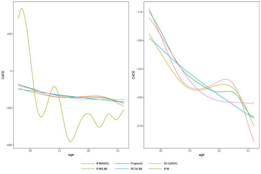
Figure 2 shows the estimated PCATEs from different methods. From the left panel in Figure 2, IPW has large variations compared to other estimators. The significantly positive estimates before age 20 conflict with the results from various established research works indicating that smoking has adverse effect on birth weights (Kramer, 1987; Almond et al., 2005; Abrevaya, 2006; Abrevaya and Dahl, 2008). From the right panel in Figure 2, the remaining four estimators show a similar pattern that the effect becomes more severe as mother’s age increases, which aligns with the existing literature (Fox et al., 1994; Walker et al., 2007). The REG(LM) estimator shows a linearly decreasing pattern, while the REG(KRR) estimator stops decreasing after age 30. For three weighted estimators, the effects are stable around age 27 to 32, but tend to decrease quickly after age 32. Compared to IPW(LM) and IPW(KRR), Proposed does not show the increasing tendency before age 30 and the decrease after age 32 is relatively smoother.
8 Discussions
The PCATE characterizes subgroup treatment effects and provides insights about how treatment effect varies across the characteristics of interest. We develop a novel nonparametric estimator for the PCATE under treatment ignorability. The proposed hybrid kernel weighting is a non-trivial extension of covariate balancing weighting in the ATE estimation literature in that it aims to achieve approximate covariate balancing for all flexible outcome mean functions and for all subgroups defined based on continuous variables. In contrast to existing estimators, we do not require any smoothness assumption on the propensity score, and thus our weighting approach is particularly useful in studies when the treatment assignment mechanism is quite complex.
We conclude with several interesting and important extensions of the current estimator as future research directions. First, an improved data-adaptive bandwidth selection procedure is worth investigating as it plays an important role in smoothing. In addition, instead of local constant regression, other alternatives such as linear or spline smoothers can be considered. Third, given the appealing theoretical properties, we will investigate efficient computation of the proposed weighting estimators with -norm. Furthermore, the asymptotic distribution of proposed estimator is worth studying so that inference procedures can be developed.
Acknowledgement
The work of Raymond K. W. Wong is partially supported by the National Science Foundation (DMS-1711952 and CCF-1934904). The work of Shu Yang is partially supported by the National Institute on Aging (1R01AG066883) and the National Science Foundation (DMS-1811245). The work of Kwun Chuen Gary Chan is partially supported by the National Heart, Lung, and Blood Institute (R01HL122212) and the National Science Foundation (DMS-1711952).
References
- Abrevaya (2006) Abrevaya, J. (2006). Estimating the effect of smoking on birth outcomes using a matched panel data approach. Journal of Applied Econometrics 21(4), 489–519.
- Abrevaya and Dahl (2008) Abrevaya, J. and C. M. Dahl (2008). The effects of birth inputs on birthweight: evidence from quantile estimation on panel data. Journal of Business & Economic Statistics 26(4), 379–397.
- Abrevaya et al. (2015) Abrevaya, J., Y.-C. Hsu, and R. P. Lieli (2015). Estimating conditional average treatment effects. Journal of Business & Economic Statistics 33(4), 485–505.
- Almond et al. (2005) Almond, D., K. Y. Chay, and D. S. Lee (2005). The costs of low birth weight. The Quarterly Journal of Economics 120(3), 1031–1083.
- Athey et al. (2016) Athey, S., G. W. Imbens, and S. Wager (2016). Approximate residual balancing: De-biased inference of average treatment effects in high dimensions. arXiv preprint arXiv:1604.07125.
- Calonico et al. (2019) Calonico, S., M. D. Cattaneo, and M. H. Farrell (2019). nprobust: Nonparametric kernel-based estimation and robust bias-corrected inference. arXiv preprint arXiv:1906.00198.
- Chan et al. (2016) Chan, K. C. G., S. C. P. Yam, and Z. Zhang (2016). Globally efficient non-parametric inference of average treatment effects by empirical balancing calibration weighting. Journal of the Royal Statistical Society. Series B, Statistical methodology 78(3), 673.
- Chernozhukov et al. (2017) Chernozhukov, V., D. Chetverikov, M. Demirer, E. Duflo, C. Hansen, W. Newey, J. Robins, et al. (2017). Double/debiased machine learning for treatment and causal parameters. Technical report.
- Einmahl et al. (2005) Einmahl, U., D. M. Mason, et al. (2005). Uniform in bandwidth consistency of kernel-type function estimators. The Annals of Statistics 33(3), 1380–1403.
- Fan et al. (2020) Fan, Q., Y.-C. Hsu, R. P. Lieli, and Y. Zhang (2020). Estimation of conditional average treatment effects with high-dimensional data. Journal of Business & Economic Statistics (just-accepted), 1–39.
- Fox et al. (1994) Fox, S. H., T. D. Koepsell, and J. R. Daling (1994). Birth weight and smoking during pregnancy-effect modification by maternal age. American Journal of Epidemiology 139(10), 1008–1015.
- Hainmueller (2012) Hainmueller, J. (2012). Entropy balancing for causal effects: A multivariate reweighting method to produce balanced samples in observational studies. Political analysis, 25–46.
- Harder and Desmarais (1972) Harder, R. L. and R. N. Desmarais (1972). Interpolation using surface splines. Journal of aircraft 9(2), 189–191.
- Imai and Ratkovic (2014) Imai, K. and M. Ratkovic (2014). Covariate balancing propensity score. Journal of the Royal Statistical Society: Series B: Statistical Methodology, 243–263.
- Kallus (2020) Kallus, N. (2020). Generalized optimal matching methods for causal inference. Journal of Machine Learning Research 21(62), 1–54.
- Kennedy (2020) Kennedy, E. H. (2020). Optimal doubly robust estimation of heterogeneous causal effects. arXiv preprint arXiv:2004.14497.
- Kramer (1987) Kramer, M. S. (1987). Intrauterine growth and gestational duration determinants. Pediatrics 80(4), 502–511.
- Lee et al. (2017) Lee, S., R. Okui, and Y.-J. Whang (2017). Doubly robust uniform confidence band for the conditional average treatment effect function. Journal of Applied Econometrics 32(7), 1207–1225.
- Mack and Silverman (1982) Mack, Y.-p. and B. W. Silverman (1982). Weak and strong uniform consistency of kernel regression estimates. Zeitschrift für Wahrscheinlichkeitstheorie und verwandte Gebiete 61(3), 405–415.
- Nie and Wager (2017) Nie, X. and S. Wager (2017). Quasi-oracle estimation of heterogeneous treatment effects. arXiv preprint arXiv:1712.04912.
- Qin and Zhang (2007) Qin, J. and B. Zhang (2007). Empirical-likelihood-based inference in missing response problems and its application in observational studies. Journal of the Royal Statistical Society: Series B (Statistical Methodology) 69(1), 101–122.
- Rosenbaum and Rubin (1983) Rosenbaum, P. R. and D. B. Rubin (1983). The central role of the propensity score in observational studies for causal effects. Biometrika 70(1), 41–55.
- Ruppert et al. (1995) Ruppert, D., S. J. Sheather, and M. P. Wand (1995). An effective bandwidth selector for local least squares regression. Journal of the American Statistical Association 90(432), 1257–1270.
- Semenova and Chernozhukov (2017) Semenova, V. and V. Chernozhukov (2017). Estimation and inference about conditional average treatment effect and other structural functions. arXiv, arXiv–1702.
- Semenova and Chernozhukov (2020) Semenova, V. and V. Chernozhukov (2020). Debiased machine learning of conditional average treatment effects and other causal functions. The Econometrics Journal.
- Van der Vaart (2000) Van der Vaart, A. W. (2000). Asymptotic Statistics, Volume 3. Cambridge university press.
- Wager and Athey (2018) Wager, S. and S. Athey (2018). Estimation and inference of heterogeneous treatment effects using random forests. Journal of the American Statistical Association 113(523), 1228–1242.
- Wahba (1990) Wahba, G. (1990). Spline Models for Observational Data. SIAM.
- Walker et al. (2007) Walker, M., E. Tekin, and S. Wallace (2007). Teen smoking and birth outcomes. Technical report, National Bureau of Economic Research.
- Wand and Jones (1994) Wand, M. P. and M. C. Jones (1994). Kernel Smoothing. Crc Press.
- Wang and Zubizarreta (2020) Wang, Y. and J. R. Zubizarreta (2020). Minimal dispersion approximately balancing weights: asymptotic properties and practical considerations. Biometrika 107(1), 93–105.
- Wasserman (2006) Wasserman, L. (2006). All of Nonparametric Statistics. Springer Science & Business Media.
- Wong and Chan (2018) Wong, R. K. and K. C. G. Chan (2018). Kernel-based covariate functional balancing for observational studies. Biometrika 105(1), 199–213.
- Zhao et al. (2019) Zhao, Q. et al. (2019). Covariate balancing propensity score by tailored loss functions. The Annals of Statistics 47(2), 965–993.
- Zheng and van der Laan (2011) Zheng, W. and M. J. van der Laan (2011). Cross-validated targeted minimum-loss-based estimation. In Targeted Learning, pp. 459–474. Springer.
- Zimmert and Lechner (2019) Zimmert, M. and M. Lechner (2019). Nonparametric estimation of causal heterogeneity under high-dimensional confounding. arXiv preprint arXiv:1908.08779.
- Zubizarreta (2015) Zubizarreta, J. R. (2015). Stable weights that balance covariates for estimation with incomplete outcome data. Journal of the American Statistical Association 110(511), 910–922.