Estimation of one-dimensional discrete-time quantum walk parameters by using machine learning algorithms
Abstract
Estimation of the coin parameter(s) is an important part of the problem of implementing more robust schemes for quantum simulation using quantum walks. We present the estimation of the quantum coin parameter used for one-dimensional discrete-time quantum walk evolution using machine learning algorithms on their probability distributions. We show that the models we have implemented are able to estimate these evolution parameters to a good accuracy level. We also implement a deep learning model that is able to predict multiple parameters simultaneously. Since discrete-time quantum walks can be used as quantum simulators, these models become important when extrapolating the quantum walk parameters from the probability distributions of the quantum system that is being simulated.
I Introduction
Quantum walks R58 ; F86 are the quantum counterparts of classical random walks, and are therefore used as the basis to generate relevant models for controlled quantum dynamics of a particle. Much like a classical random walk, the formalism for quantum walks has also developed in two forms - the discrete-time quantum walk (DTQW) and the continuous-time quantum walk (CTQW). Both the formalisms exhibit features that enable them to effectively realise quantum computational tasks DW08 ; C09 ; A07 ; MSS07 ; BS06 ; FGG07 ; K08 . Quantum superposition and interference have the effect of allowing the quantum walker to have a quadratically faster spread in position space in comparison to a classical walker P88 ; ADZ93 ; M96 ; K03 ; CCD03 ; CG04 ; VA12 . This has applications in modelling dynamics of several quantum systems, like quantum percolation CB14 ; KKNJ12 ; CAC19 , energy transport in photosynthesis ECR07 ; MRLA08 , graph isomorphism DW08 , quantum algorithms CMC20 ; PMCM13 , and even in generating a scheme for universal quantum computation SCSC19 ; SCASC20 .
Much like a classical walk, the dynamics of a walker undergoing CTQW can be described only by a position Hilbert space, whereas a walker performing DTQW requires an additional degree of freedom to express its controlled dynamics. This is realised by the coin Hilbert space, which is an internal state of the walker, and provides the relevant additional degree of freedom for the walker. Tuning the parameters and evolution operators of a DTQW enables the walker to simulate several quantum mechanical phenomena, such as topological phases COB15 ; SRFL08 ; KRBD10 ; AO13 , relativistic quantum dynamics S06 ; CBS10 ; MC16 ; C13 ; MBD13 ; MBD14 ; AFF16 ; P16 ; RLBL05 , localization J12 ; C12 ; CB15 , and neutrino oscillations MMC17 ; MP16 . Quantum walks have been experimentally implemented in various physical systems, such as photonic systems SCP10 ; BFL10 ; P10 , nuclear magnetic resonance systems RLBL05 , trapped ion systems SRS09 ; ZKG10 , and cold atoms KFCSWMW09 .
It is known that the coin parameters of a quantum walk play a significant role in determining the overall dynamics of the system. For instance, the coin parameters of a split-step quantum walk determine topological phases COB15 ; SRFL08 ; KRBD10 , neutrino oscillation MMC17 ; MP16 , and the mass of a Dirac particle MC16 . Thus the coin parameter is an important piece of the puzzle while using a quantum walk as a quantum simulation scheme. It thus becomes a crucial problem to be able to estimate the parameters of a quantum walk in order to facilitate better quantum simulations and also for further research into modelling realistic quantum dynamics.
In this regard, the problem partially becomes one of finding a pattern hidden in this complex data, and an effective approach is to use an algorithm that automates its learning process. In this context, the term ’learning’ aptly described in Mitchell97 : A computer program is said to learn from experience E with respect to some class of tasks T and performance measure P, if its performance at tasks in T, as measured by P, improves with experience E. The task T in this particular case is defined as, to output a function , such that the input vector corresponds to the known probability distribution after steps and the output corresponds to the parameter . It may, however, be noted that due to the No Free Lunch theorem W96 , the machine learning strategies for different types of quantum walks are not likely to be the same as for this particular case.
It is known that the Quantum Fisher Information (QFI) P11 ; TP13 ; S13 ; TA14 of a quantum walker’s position quantifies a bound to the amount of information that can be extracted from the probability distribution P12 ; SCP19 . It has also been shown that it is indeed possible to estimate the coin parameter of a DTQW with a single-parameter coin. However, the approaches that rely on QFI to predict the parameters in a DTQW share a similar constraint, viz, even though is a continuous, single-valued function over , the variations in the plot are small, and thus contribute to the error in determining SCP19 . In this work, we train various machine learning models and demonstrate that such models can indeed estimate the quantum walk parameters to a good accuracy. We also estimate the coin parameter and the number of steps for a DTQW simultaneously with a multilayer perceptron model, and demonstrate that it performs much better than a baseline model that does not learn with experience.
This paper is structured as follows. In section II we introduce a standard DTQW, an SSQW, and describe the evolution operators that determine their dynamics. We give a brief overview of the machine learning models used and their parameters in Section III. Section IV details our results of training the machine learning algorithms and their performance. We wrap up the paper in section V with a small discussion on our results and conclusions drawn.
II Discrete-time quantum walk
The evolution of a walker executing DTQW is defined in a Hilbert space , where and are the walker’s coin and position Hilbert spaces, respectively. The coin Hilbert space has the basis states , and the position Hilbert space is defined by the basis states , where . The evolution is described by two unitary operators, known as the coin and shift operations. The coin operator affects the coin Hilbert space, and the shift operator evolves the walker in a superposition of position states, the amplitudes of which are determined by the coin operation. In case of the one-dimensional DTQW, the most general unitary coin operator is an matrix, which has three independent parameters. That said, even one- and two-parameter coins are very useful while simulating various systems. As an example, the single-parameter split step DTQW is very effective to simulate neutrino oscillations MMC17 , topological phases COB15 , and the Dirac equation MC16 .
In a one-dimensional DTQW, the coin operation is an matrix, defined as,
| (1) |
The shift operation is defined as,
| (2) |
The initial internal state of the walker is defined as,
| (3) |
and the complete evolution equation will be in the form,
| (4) |
where is the number of steps taken by the walker.
To obtain the the one-parameter coin form from Eq. (1), we fix the values and . This is the convention adopted in the remainder of this text. The one-parameter coin operator is thus given as,
| (5) |
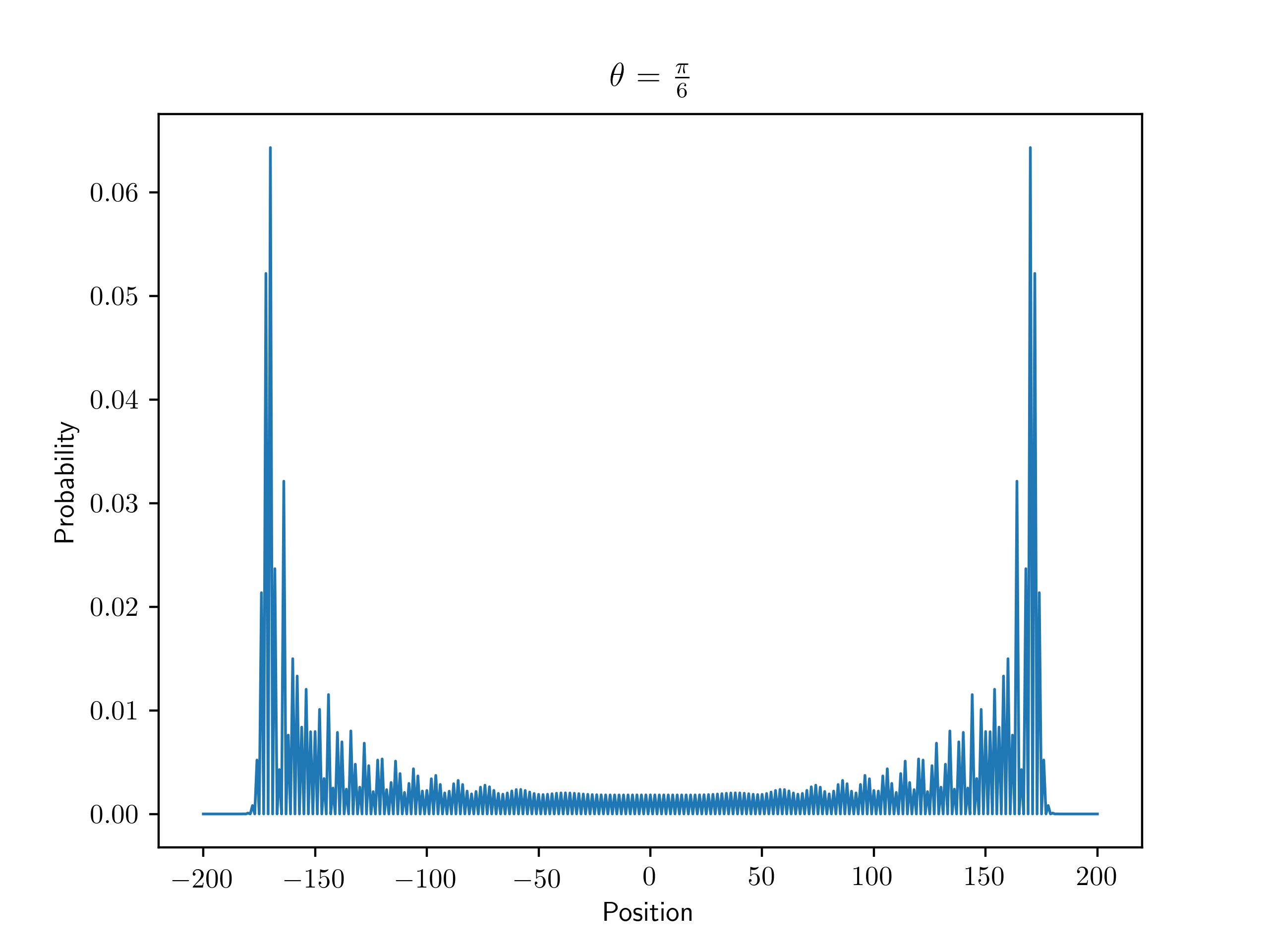
Fig. 1 shows the probability distributions in position space of a walker performing a DTQW with different values of as in Eq. (5).
 |
 |
| (a) | (b) |
 |
 |
| (c) | (d) |
A special case of a DTQW is the split-step quantum walk (SSQW), in which case the evolution operator is given by a composition of two half-steps,
| (6) |
Where represent the two coin operations, which are defined in the same form as in Eq. (5), and are directed shift operations, defined as,
| (7) |
In a one-dimensional visualisation, an SSQW implements the case when the components that are in the direction of experience a different coin () than the components in the direction, which experience the coin . The evolution of the walk is still in the form as shown in Eq. (4), with the appropriate walk operator substituted from Eq. (6).
Fig. 2 shows the probability distributions obtained by a walker executing a SSQW with multiple combinations of and . Unlike the two peak probability distribution from the single coin DTQW, SSQW can results in four peak probability distribution.
 |
 |
| (a) | (b) |
 |
 |
| (c) | (d) |
III A brief note on machine learning
Machine learning was originally created to try and create solutions to problems which were hard to define formally, such as recognizing faces in images, or cognition of spoken words. This necessitated the creation of algorithms that could learn from experience of examples supplied to them, so the programmer was absolved of the requirement to formally specify all knowledge needed to solve the problem beforehand.
While the hardcoded knowledge methods worked very well for small, relatively sterile environments such as the world of chess CHH02 , such programs face difficulties in subjective and intuitive tasks such as understanding speech or object recognition. Inference-based methods have been suggested and implemented as a possible solution to this type of problem, but have not had much success LG89 ; D15 . Modern approaches circumvent this difficulty by implementing algorithms that have the capability of recognising patterns in raw data on their own GBC16 - a trait now known as machine learning.
Linear regression
Linear regression takes an input vector of features and outputs a vector , which is to be interpreted as a prediction for the actual vector . The model is named linear regression as it attempts to find a linear function from the input vector to the output. More mathematically, linear regression models calculate the prediction as
| (8) |
where is a matrix of weights and is known as the bias vector. The weight essentially determines how the feature affects the prediction . The bias vector is the value that this function tends to take in the absence of an input, and thus ensures that the mapping of features to predictions is an affine function.
Ridge regression
Due to the large sizes of the input vectors, a case may arise where the input variables may have near-linear relationships, a phenomenon known as multicollinearity B07 . Multicollinearity leads to unbiased linear regression estimates, but with high variances. Ridge regression is a method to improve estimation by adding a small amount of bias M98 .
Assume that one requires the estimates of a vector , as in Eq. (8). A traditional linear regression-based method would seek to minimize the sum of squared residuals , where represents the Euclidean norm. Ridge regression introduces a regularization term in this in order to guide the solution towards preferred properties. Thus, the final minimization looks like,
| (9) |
Nearest-neighbour regression
The -Nearest Neighbour algorithm was proposed as a nonparametric method for pattern recognition, and is used for both classification and regression analyses CH67 ; A92 . In our case, the task is that of regression, and therefore the output is the average of k closest examples in the feature space of the training set. The algorithm proceeds as follows:
-
1.
Load the training data and initialize to the chosen number of neighbours.
-
2.
For each example in the training data,
-
(a)
Calculate the distance between the query and the current example from the data.
-
(b)
Add the distance and index of this example to an ordered collection
-
(a)
-
3.
Sort the ordered collection in ascending order of distances.
-
4.
Pick the labels of first entries in this collection, and return the mean of the these labels.
This algorithm defers all computation until function evaluation, and only locally approximates the said function. Thus it is also a valid example of instance-based learning PE20 ; H01 . As it uses the training examples in the local neighbourhood of the query to generate a prediction, it is extremely sensitive to the local structure of the data BGRS99 . Since only the closest training examples nearest to a query are considered to generate the prediction for it, this algorithm does not require an explicit training step.
Multilayer Perceptron Models
Multilayer perceptron (MLP) models are a class of artificial neural networks, which are algorithms modelled after biological neural networks in animal brains MP43 ; K56 . These algorithms learn by example, and consist of units known as neurons, which are loosely modelled after their biological counterparts. Fig. 3 shows a basic MLP model with 3 neurons in the input layer, 2 hidden layers of four neurons each, and an output layer of 3 neurons. In this paper, the MLP model used has 200 neurons in the input layer, 200 in the hidden layer, and 2 in the output layer. The input and hidden layer neurons use a rectified linear unit (ReLU) as their activation function, and the output layer uses an exponential activation function.
 |
 |
| (a) | (b) |
The goal of this model is to approximate a function by creating a mapping and then learning the parameters so that approximates as closely as possible. This is a type of feedforward model GBC16 , as there are no inputs that are fed back to the input from the output of the model. The model is provided a certain amount of labelled examples, which consist of both the input and the output (also known as the training set). The model uses these to tweak the parameters the best it can, and then predicts corresponding to unlabelled values of (also known as the testing set). This technique is known as supervised learning.
Our MLP model uses the cross-entropy between training data and the predictions made by the model as the cost function, and attempts to minimize it via an optimized gradient descent method. In our model, the optimizer used is Nadam. The Nadam (Nesterov-accelerated Adaptive Moment estimation) computes adaptive learning rates for each parameter by combining the approaches of Nesterov accelerated gradients and adaptive moment estimation algorithms D16 ; N83 ; KB15 ; R17 .
Performance metric
We measure the performance of our model by computing the mean square error of the model on the testing set, defined as,
| (10) |
where is the number of elements in the testing set, and is the length of the output vector. Eq. (10) may also be written in terms of Euclidean distance,
| (11) |
of the predicted values and the actual values of . It is important to note here that the error is considered over the testing set and not the training set.
IV Results
In this work, we have used machine learning algorithms and trained an MLP model in an attempt to estimate the parameters of a one-dimensional DTQW. The models were trained on DTQW with , and varying from to , at an interval of . The dataset consists of DTQW distributions that resulted after using these parameters in conjunction with a symmetric initial state as,
| (12) |
We have chosen the ratio of training to testing data as () for this dataset. As a result, randomly selected probability distributions are used to train our algorithm, and the rest are used to test its performance. Three regression models, namely, K-nearest neighbours, linear regression and ridge regression, were trained on this data, and their performance was evaluated by the mean square error (MSE) of their predictions. The results are shown as in Table 1. It is observed that while all the models return a very low MSE, but the performance of the linear regression model is a few orders of magnitude better than the next best performing model (k-nearest neighbours).
| Model | Mean-squared error |
|---|---|
| Linear Regression | 2.501 x |
| K-Nearest Neighbours (k = 5) | 2.058 x |
| Ridge Regression ( = 0.01) | 2.783 x |
Using the same training data as specified above, the model was tasked to predict the value of , and given the testing data corresponding to , which is outside the range used to generate the training data. Table 2 details the predictions by each of these models.
| Model | Expected | Predicted | Error (%) |
|---|---|---|---|
| Linear Regression | 0.048% | ||
| K-Nearest Neighbours (k = 5) | 0.046% | ||
| Ridge Regression ( = 0.01) | 0.401% |
We also implemented an MLP model (detailed in section III) to try and predict two parameters ( and ) of a 1D-DTQW simultaneously via deep learning. The model contains layers, out of which there is hidden layer. The model uses rectified linear units as the activation function for the first two layers (i.e. the input and hidden layers, respectively), and an exponential activation for the output layer. The neural net uses the Nadam optimizer. Other possible optimizers that can be used here are AdaGrad, AdaDelta and Adam. AdaGrad offers the benefit of eliminating the need of manually tuning the learning rate, but has the weakness that it accumulates a sum of squared gradients in its denominator over time, causing the learning rate to shrink and eventually become infinitesimally small, and the algorithm stop learning at this point. AdaDelta aims to reduce the aggressive decay of the learning rate in AdaGrad by fixing a window size of the accumulated past gradients. Adam tries to improve on both AdaGrad and AdaDelta by considering an exponentially decaying average of past gradients to adjust its learning rates. Nadam, however, improves on the performance of Adam by using Nesterov-accelerated gradients, and was chosen as the best fit for this case.
To train this network, we generated a new dataset, which contained all possible combinations of the parameters and , varying between and respectively, with a step size of for , and for . The dataset thus comprised of different probability distributions. The training-testing split was chosen to be the same as the earlier case (), and the training set thus consisted of a randomly selected probability distributions of the total.
In order to judge the effectiveness of this model, we also designed a baseline model, which would always predict the mean of all supplied training values of and ( and respectively, for this case), for any input distribution. The MSE from this baseline model was found to be .
Our neural network gave an output MSE of , which is a reduction of on the baseline error. This proves that the neural network is able to effectively learn and reproduce the patterns found in the DTQW probability distributions in order to reasonably estimate both the parameters of a 1D-DTQW.
We also tried to estimate selected parameters of an SSQW. A one-dimensional SSQW with two single-parameter coins as defined in Eq. (5) which typically has 3 parameters, , , and . For the purposes of this task, we varied in the range at an interval of , while keeping , and fixed. We trained a linear regression model on this data, as well as a K-nearest neighbour model. The parameter was estimated with a good accuracy, as is seen from the contents of Table 3.
| Model | Mean-squared error |
|---|---|
| K-Nearest Neighbour (k = 5) | |
| Linear Regression |
V Conclusions
In this work, we have demonstrated the effectiveness of machine learning models while estimating the coin parameter in a DTQW and an SSQW. We have applied these models on the one-dimensional DTQW and SSQW, and attempted to estimate the parameters from these walks.
In the case of DTQW, we applied three different models in order to estimate the coin parameter , and conclude that a machine learning-based approach is indeed able to estimate the parameter very well. We also attempt to use a neural network in order to try and predict the two parameters at once, and show that its prediction error reduces by a significant amount from the baseline error, implying that the network is able to distinguish and replicate patterns found in this data. We also use two different models in order to estimate one of the coin parameters of a SSQW.
It is important to keep in mind that the accuracy of the predictions will vary with the amount of training data it is given. Typically, larger datasets improve the accuracy. The accuracy is also very dependent on the model itself under consideration. There is no single known machine learning algorithm that may outperform all others, and it is thus important to choose the algorithm for implementation with care.
Acknowledgment: CMC would like to thank Department of Science and Technology, Government of India for the Ramanujan Fellowship grant No.:SB/S2/RJN-192/2014. We also acknowledge the support from Interdisciplinary Cyber Physical Systems (ICPS) programme of the Department of Science and Technology, India, Grant No.:DST/ICPS/QuST/Theme-1/2019/1 and US Army ITC-PAC contract no. FA520919PA139.
References
- (1) G. V. Riazanov, “The Feynman path integral for the Dirac equation”, Zh. Eksp. Teor. Fiz. 33, 1437 (1958), [Sov. Phys. JETP 6, 1107-1113 (1958)].
- (2) R. P. Feynman,“Quantum mechanical computers”, Found. Phys. 16, 507-531 (1986).
- (3) B. L. Douglas and J. B. Wang, “A classical approach to the graph isomorphism problem using quantum walks,” J. Phys. A: Math. Theor. 41, 7, 075303 (2008)
- (4) A. M. Childs, “Universal computation by quantum walk,” Phys. Rev. Lett. 102, 18, 180501 (2009).
- (5) A. Ambainis, “Quantum walk algorithm for element distinctness,” SIAM J. Comput. 37 (1), pp. 210–239 (2007).
- (6) F. Magniez, M. Santha, and M. Szegedy, “Quantum algorithms for the triangle problem,” SIAM J. Comput. 37, no. 2, pp. 413–424 (2007).
- (7) H. Buhrman and R. Spalek, “Quantum verification of matrix products,” Proceedings of the annual ACM-SIAM SODA, pp. 880–889 (2006).
- (8) E. Farhi, J. Goldstone, and S. Gutmann, “A quantum algorithm for the Hamiltonian NAND tree,” arXiv:quant-ph/0702144 (2007).
- (9) N. Konno, “Quantum walks,” Quantum potential theory, pp. 309–452, Springer (2008).
- (10) K. R. Parthasarathy, “The passage from random walk to diffusion in quantum probability,” J. App. Prob. 25, pp. 151–166, 1988.
- (11) Y. Aharonov, L. Davidovich, and N. Zagury, “Quantum random walks,” Phys. Rev. A 48, 1687-1690 (1993).
- (12) D. A. Meyer, “From quantum cellular automata to quantum lattice gases,” J. Stat. Phys. 85, no. 5-6, pp. 551–574 (1996).
- (13) J. Kempe, “Quantum random walks: an introductory overview”, Contemp. Phys 44.4, 307-327 (2003).
- (14) S. E. Venegas-Andraca, “Quantum walks: a comprehensive review”, Quantum. Info. Process 11, 1015 (2012).
- (15) A. M. Childs, R. Cleve, E. Deotto, E. Farhi, S. Gutmann, and D. A. Spielman, “Exponential algorithmic speedup by a quantum walk,” Proceedings of the annual ACM symposium on Theory of computing, pp. 59–68, ACM (2003).
- (16) A. M. Childs and J. Goldstone, “Spatial search by quantum walk,” Phys. Rev. A 70 2, 022314 (2004).
- (17) C. Chandrashekar and T. Busch, “Quantum percolation and transition point of a directed discrete-time quantum walk,” Sci. rep., 4, 6583 (2014).
- (18) B. Kollár, T. Kiss, J. Novotnỳ, and I. Jex, “Asymptotic dynamics of coined quantum walks on percolation graphs,” Phys. Rev. Let. 108 23, 230505 (2012)
- (19) P. Chawla, C. V. Ambarish, C. M. Chandrashekar, “Quantum percolation in quasicrystals using continuous-time quantum walk,” J.Phys. Comm. 3, 125004, (2019).
- (20) G. S. Engel, T. R. Calhoun, E. L. Read, T.-K. Ahn, T. Manc̆al, Y.-C. Cheng, R. E. Blankenship, and G. R. Fleming, “Evidence for wavelike energy transfer through quantum coherence in photosynthetic systems,” Nat., 446, 7137, (2007).
- (21) M. Mohseni, P. Rebentrost, S. Lloyd, and A. Aspuru Guzik, “Environment-assisted quantum walks in photosynthetic energy transfer,” J. Chem. Phys. 129, 174106 (2008).
- (22) P. Chawla, R. Mangal, C. M. Chandrashekar, “Discrete-time quantum walk algorithm for ranking nodes on a network,” Quantum Inf. Proc. 19, 158 (2020).
- (23) G. Paparo, M. Müller, F. Comellas, M. A. Martin-Delgado, “Quantum Google in a Complex Network,” Sci. Rep. 3, 2773 (2013).
- (24) S. Singh, P. Chawla, A. Sarkar, C. M. Chandrashekar, “Computational power of single qubit discrete-time quantum walk,” arXiv:1907.04084. (2019).
- (25) S. Singh, P. Chawla, A. Agarwal, S. Srinivasan, C. M. Chandrashekar, “Universal quantum computation using single qubit discrete-time quantum walk,” arXiv:2004.05956 (2020)..
- (26) C. M. Chandrashekar, H. Obuse, T. Busch, “Entanglement properties of localized states in 1D topological quantum walks,” arXiv:1502.00436 [quant-ph] (2015)..
- (27) A. P. Schnyder, S. Ryu, A. Furusaki, A. W. W. Ludwig, “Classification of topological insulators and superconductors in three spatial dimensions,” Phys. Rev. B 78, 195125 (2008).
- (28) T. Kitagawa, M. Rudner, E. Berg, E. Demler, “Exploring Topological Phases with quantum walks,” Phys. Rev. A 82, 033429 (2010).
- (29) J. K. Asbóth , H. Obuse, “Bulk-boundary correspondence for chiral symmetric quantum walks,” Phys. Rev. B 88, 121406(R) (2013).
- (30) F. W. Strauch, “Relativistic quantum walks,” Phys. Rev. A 73 5, 054302, (2006).
- (31) C. Chandrashekar, S. Banerjee, and R. Srikanth, “Relationship between quantum walks and relativistic quantum mechanics,” Phys. Rev. A 81, 6, 062340, (2010).
- (32) A. Mallick, C. M. Chandrashekar, “Dirac cellular automaton from split-step quantum walk,” Sci. Rep. 6, 25779 (2016).
- (33) C. M. Chandrashekar, “Two-component dirac-like hamiltonian for generating quantum walk on one-, two-and three-dimensional lattices,” Sci. Rep. 3, 2829 (2013).
- (34) G. Di Molfetta, M. Brachet, and F. Debbasch, “Quantum walks as massless dirac fermions in curved space-time,” Phys. Rev. A 88, 4, 042301 (2013).
- (35) G. Di Molfetta, M. Brachet, and F. Debbasch, “Quantum walks in artificial electric and gravitational fields,” Phys. A: Stat. Mech. App 397, pp. 157–168 (2014).
- (36) P. Arrighi, S. Facchini, and M. Forets, “Quantum walking in curved spacetime,” Quantum Inf. Proc. 15, 8, pp. 3467–3486 (2016).
- (37) A. Pèrez, “Asymptotic properties of the dirac quantum cellular automaton,” Phys. Rev. A 93, 1, 012328 (2016).
- (38) C. A. Ryan, M. Laforest, J.-C. Boileau, and R. Laflamme, “Experimental implementation of a discrete-time quantum random walk on an NMR quantum-information processor,” Phys. Rev. A 72 , 062317 (2005).
- (39) A. Joye, “Dynamical localization for d-dimensional random quantum walks,” Quantum Inf. Proc. 11, 5, 1251–1269 (2012).
- (40) C. M. Chandrashekar, “Disorder induced localization and enhancement of entanglement in one-and two-dimensional quantum walks,” arXiv:1212.5984 (2012).
- (41) C. Chandrashekar and T. Busch, “Localized quantum walks as secured quantum memory,” EuroPhys. Lett., 110, 1, 10005 (2015).
- (42) A. Mallick, S. Mandal, and C. Chandrashekar, “Neutrino oscillations in discrete-time quantum walk framework,” J. Eur. Phys. C 77, 2, 85 (2017).
- (43) G. Di Molfetta and A. Pèrez, “Quantum walks as simulators of neutrino oscillations in a vacuum and matter,” N. J. Phys. 18, 10, 103038 (2016).
- (44) A. Schreiber, K. N. Cassemiro, V. Potocek, A. Gabris, P. J. Mosley, E. Andersson, I. Jex, Ch. Silberhorn, “Photons Walking the Line: A quantum walk with adjustable coin operations,” Phys. Rev. Lett. 104, 050502 (2010).
- (45) M. A. Broome, A. Fedrizzi, B. P. Lanyon, I. Kassal, A. Aspuru-Guzik, & A. G. White, “Discrete Single-Photon Quantum Walks with Tunable Decoherence,” Phys. Rev. Lett. 104, 153602 (2010).
- (46) A. Peruzzo et. al , “Quantum Walks of Correlated Photons,” Science 329, 1500 (2010).
- (47) H. Schmitz, R. Matjeschk, Ch. Schneider, J. Glueckert, M. Enderlein, T. Huber, & T. Schaetz,“ Quantum walk of a trapped ion in phase space,” Phys. Rev. Lett 103, 090504 (2009).
- (48) F. Zahringer, G. Kirchmair, R. Gerritsma, E. Solano, R. Blatt, C. F. & Roos, “Realization of a Quantum Walk with One and Two Trapped Ions,” Phys. Rev. Lett 104, 100503 (2010).
- (49) M. Karski, L. F‘̀orster, J-M. Choi, A. Steffen, W. Alt, D. Meschede, A. & Widera, “Quantum Walk in Position Space with Single Optically Trapped Atoms,” Science 325, 5937, 174-177 (2009).
- (50) T. Mitchell, “Machine Learning.” McGraw-Hill, New York, New York, 1997.
- (51) D. H. Wolpert, “The Lack of A Priori Distinctions Between Learning Algorithms,” Neur. Comput. 8 (7), 1341-1390 (1996).
- (52) M. G. A. Paris, “Quantum Estimation for Quantum Technology“, Int. J. Quant. Inf. 07 (supp01), 125–137 (2009).
- (53) G. Tóth, D. Petz, “Extremal properties of the variance and the quantum Fisher information“. Phys. Rev. A 87, 3, 032324 (2013).
- (54) Yu, Sixia, “Quantum Fisher Information as the Convex Roof of Variance“. arXiv:1302.5311 (2013).
- (55) G. Tóth, I. Apellaniz,“Quantum metrology from a quantum information science perspective“. J. Phys. A: Math. Theor. 47, 42 424006 (2014).
- (56) P. Hyllus, “Fisher information and multiparticle entanglement“. Phys. Rev. A 85, 2, 022321 (2012).
- (57) S. Singh, C. M. Chandrashekar, M. G. A. Paris, “Quantum walker as a probe for its coin parameter” Phys. Rev. A 99, 052117 (2019).
- (58) M. Campbell, A.J. Hoane Jr., F. Hsu. “Deep Blue,” Art. Int. 134 1-2, pp 54-83 (2002).
- (59) D. B. Lenat, R. V. Guha, “Building Large Knowledge-Based Systems; Representation and Inference in the Cyc Project” (1st ed.). Boston, MA, USA: Addison-Wesley Longman Publishing Co., Inc. (1989).
- (60) P. Domingos, “The Master Algorithm: How the Quest for the Ultimate Learning Machine Will Remake Our World,” New York, New York, Basic Books (2015)
- (61) I. Goodfellow, Y. Bengio, A. Courville, “Deep Learning”, MIT Press, MA, USA (2016).
- (62) R. M. O‘Brien, “A Caution Regarding Rules of Thumb for Variance Inflation Factors“. Qual. Quant. 41, 673–690. (2007).
- (63) M. Gruber, “Improving Efficiency by Shrinkage: The James–Stein and Ridge Regression Estimators.” Boca Raton: CRC Press. (1998).
- (64) A. N. Tikhonov, “Solution of incorrectly formulated problems and the regularization method.” Dokl. Akad. Nauk SSSR 151, 3, 501-504 (1963).
- (65) A. N. Tikhonov, A. Goncharsky, V. V. Stepanov, A. G. Yagola, “Numerical Methods for the Solution of Ill-Posed Problems”. Netherlands: Springer Netherlands (1995).
- (66) R. Tibshirani, “Regression Shrinkage and Selection via the lasso,” J. R. Stat. Soc. Ser. B (meth.) 58 , 1 267–88 (1996).
- (67) T. M. Cover, P. E. Hart, “Nearest neighbor pattern classification,” IEEE Trans. Inf. Theor. 13, 1, 21–27 (1967).
- (68) N. S. Altman, “An introduction to kernel and nearest-neighbor nonparametric regression,” Amer. Stat. 46, 3, 175–185 (1992).
- (69) S. M. Piryonesi, T. E. El-Diraby, “Role of Data Analytics in Infrastructure Asset Management: Overcoming Data Size and Quality Problems,” J. Trans. Engg. Part B: Pavements 146, 2, 04020022 (2020).
- (70) T. Hastie, R. Tibshirani, J. H. Friedman, “The elements of statistical learning : data mining, inference, and prediction,” Springer, New York (2001).
- (71) K. Beyer, J. Goldstein, R. Ramakrishnan, U. Shaft, “When Is ’Nearest Neighbor‘ Meaningful?” ICDT 1999, Lec. Notes in Comp. Sc. 1540 Springer, Berlin, Heidelberg (1999).
- (72) W. McCulloch, W. Pitts, “A Logical Calculus of Ideas Immanent in Nervous Activity,” Bull. Math. Biophy. 5, 4, 115–133 (1943).
- (73) S. C. Kleene, “Representation of Events in Nerve Nets and Finite Automata,” Ann. Math. St. 34 (Automata Studies), Princeton University Press, pp. 3–42 (1956).
- (74) T. Dozat, “Incorporating Nesterov Momentum into Adam,” Proceedings of the ICLR Workshop, (2016).
- (75) Yurii Nesterov, “A method for unconstrained convex minimization problem with the rate of convergence (1/),” Dok. ANSSSR (trans. Soviet. Math. Docl.) 269 pp. 543–547 (1983).
- (76) D. P. Kingma, J. L. Ba, “Adam: A Method for Stochastic Optimization.” ICLR Conf. Proc., pp. 1–13 (2015).
- (77) S. Ruder, “An overview of gradient descent optimization algorithms”, arXiv:1609.04747 [cs.LG] (2016)