Estimation and inference for the Wasserstein distance between mixing measures in topic models
Abstract
The Wasserstein distance between mixing measures has come to occupy a central place in the statistical analysis of mixture models. This work proposes a new canonical interpretation of this distance and provides tools to perform inference on the Wasserstein distance between mixing measures in topic models. We consider the general setting of an identifiable mixture model consisting of mixtures of distributions from a set equipped with an arbitrary metric , and show that the Wasserstein distance between mixing measures is uniquely characterized as the most discriminative convex extension of the metric to the set of mixtures of elements of . The Wasserstein distance between mixing measures has been widely used in the study of such models, but without axiomatic justification. Our results establish this metric to be a canonical choice. Specializing our results to topic models, we consider estimation and inference of this distance. Although upper bounds for its estimation have been recently established elsewhere, we prove the first minimax lower bounds for the estimation of the Wasserstein distance between mixing measures, in topic models, when both the mixing weights and the mixture components need to be estimated. Our second main contribution is the provision of fully data-driven inferential tools for estimators of the Wasserstein distance between potentially sparse mixing measures of high-dimensional discrete probability distributions on points, in the topic model context. These results allow us to obtain the first asymptotically valid, ready to use, confidence intervals for the Wasserstein distance in (sparse) topic models with potentially growing ambient dimension .
keywords:
1 Introduction
This work is devoted to estimation and inference for the Wasserstein distance between the mixing measures associated with mixture distributions, in topic models.
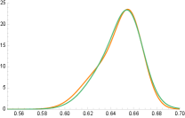
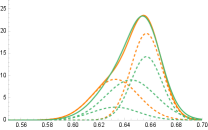
Our motivation stems from the general observation that standard distances (Hellinger, Total Variation, Wasserstein) between mixture distributions do not capture the possibility that similar distributions may arise from mixing completely different mixture components, and have therefore different mixing measures. Figure 1 illustrates this possibility.
In applications of mixture models in sciences and data analysis, discovering differences between mixture components is crucial for model interpretability. As a result, the statistical literature on finite mixture models largely focuses on the underlying mixing measure as the main object of interest, and compares mixtures by measuring distances between their corresponding mixing measures. This perspective has been adopted in the analysis of estimators for mixture models [42, 49, 31, 17, 48], in Bayesian mixture modeling [45, 44], and in the design of model selection procedures for finite mixtures [47]. The Wasserstein distance is a popular choice for this comparison [49, 31], as it is ideally suited for comparing discrete measures supported on different points of the common space on which they are defined.
Our first main contribution is to give an axiomatic justification for this distance choice, for any identifiable mixture models.
Our main statistical contribution consists in providing fully data driven inferential tools for the Wasserstein distance between mixing measures, in topic models. Optimal estimation of mixing measures in particular mixture models is an area of active interest (see, e.g., [42, 49, 31, 17, 48, 35, 69]).
In parallel, estimation and inference of distances between discrete distributions has begun to receive increasing attention [30, 65].
This work complements both strands of literature and we provide solutions to the following open problems:
(i) Minimax lower bounds for the estimation of the Wasserstein distance between mixing measures in topic models, when both the mixture weights and the mixture components are estimated from the data;
(ii) Fully data driven inferential tools for the Wasserstein distance between topic-model based, potentially sparse, mixing measures.
Our solution to (i) complements recently derived upper bounds on this distance [8], thereby confirming that near-minimax optimal estimation of the distance is possible, while the inference problem (ii), for topic models, has not been studied elsewhere, to the best of our knowledge. We give below specific necessary background and discuss our contributions, as well as the organization of the paper.
2 Our contributions
2.1 The Sketched Wasserstein Distance (SWD) between mixture distributions equals the Wasserstein distance between their mixing measures
Given a set of probability distributions on a Polish space , consider the set of finite mixtures of elements of . As long as mixtures consisting of elements of are identifiable, we may associate any with a unique mixing measure , which is a probability measure on .
We assume that is equipped with a metric . This may be one of the classic distances on probability measures, such as the Total Variation (TV) or Hellinger distance, or it may be a more exotic distance, for instance, one computed via a machine learning procedure or tailored to a particular data analysis task. As mentioned above, given mixing measures and , corresponding to mixture distributions and , respectively, it has become common in the literature to compare them by computing their Wasserstein distance with respect to the distance (see, e.g., [49, 31]). It is intuitively clear that computing a distance between the mixing measures will indicate, in broad terms, the similarity or dissimilarity between the mixture distributions; however, it is not clear whether using the Wasserstein distance between the mixing measures best serves this goal, nor whether such a comparison has any connection to a bona fide distance between the mixture distributions themselves.
As our first main contribution, we show that, indeed, the Wassersetin distance between mixing measures is a fundamental quantity to consider and study, but we arrive at it from a different perspective. In Section 3 we introduce a new distance, the Sketched Wasserstein Distance () on , between mixture distributions which is defined and uniquely characterized as the largest—that is, most discriminative—jointly convex metric on for which the inclusion is an isometry. Despite the abstractness of this definition, we show, in Theorem 1 below that
This fact justifies our name Sketched Wasserstein Distance for the new metric—it is a distance on mixture distributions that reduces to a Wasserstein distance between mixing measures, which may be viewed as “sketches” of the mixtures. We use the results of Section 3 as further motivation for developing inferential tools for the Wasserstein distance between mixing measures, in the specific setting provided by topic models. We present this below.
2.2 Background on topic models
To state our results, we begin by introducing the topic model, as well as notation that will be used throughout the paper. We also give in this section relevant existing estimation results for the model. They serve as partial motivation for the results of this paper, summarized in the following sub-sections.
Topic models are widely used modeling tools for linking discrete, typically high dimensional, probability vectors. Their motivation and name stems from text analysis, where they were first introduced [13], but their applications go beyond that, for instance to biology [15, 18]. Adopting a familiar jargon, topic models are used to model a corpus of documents, each assumed to have been generated from a maximum of topics. Each document is modeled as a set of words drawn from a discrete distribution supported on the set of words , where is the dictionary size. One observes independent, -dimensional word counts for and assumes that
| (1) |
For future reference, we let denote the associated word frequency vector.
The topic model assumption is that the matrix , with columns , the expected word frequencies of each document, can be factorized as , where the matrix has columns in the probability simplex , corresponding to the conditional probabilities of word occurrences, given a topic. The matrix collects probability vectors with entries corresponding to the probability with which each topic is covered by document , for each . The only assumption made in this factorization is that is common to the corpus, and therefore document independent: otherwise the matrix factorization above always holds, by a standard application of Bayes’s theorem. Writing out the matrix factorization one column at a time
| (2) |
one recognizes that each (word) probability vector is a discrete mixture of the (conditional) probability vectors , with potentially sparse mixture weights , as not all topics are expected to be covered by a single document . Each probability vector can be written uniquely as in (2) if uniqueness of the topic model factorization holds. The latter has been the subject of extensive study and is closely connected to the uniqueness of non-negative matrix factorization. Perhaps the most popular identifiability assumption for topic models, owing in part to its interpretability and constructive nature, is the so called anchor word assumption [25, 4], coupled with the assumption that the matrix has rank . We state these assumptions formally in Section 4.1. For the remainder of the paper, we assume that we can write uniquely as in (2), and refer to as the true mixture weights, and to , , as the mixture components. Then the collection of mixture components defined in the previous section becomes and the mixing measure giving rise to is
which we view as a probability measure on the metric space obtained by equipping with a metric .
Computationally tractable estimators of the mixture components collected in have been proposed by [4, 3, 61, 54, 9, 10, 67, 38], with finite sample performance, including minimax adaptive rates relative to and obtained by [61, 9, 10]. In Section 4.1 below we give further details on these results.
In contrast, minimax optimal, sparsity-adaptive estimation of the potentially sparse mixture weights has only been studied very recently in [8]. Given an estimator with for all , this work advocates the usage of an MLE-type estimator ,
| (3) |
If were treated as known, and replaced by , the estimator in (3) reduces to , the MLE of under the multinomial model (1).
Despite being of MLE-type, the analysis of , for , is non-standard, and [8] conducted it under the general regime that we will also adopt in this work. We state it below, to facilitate contrast with the classical set-up.
| Classical Regime | General Regime | |
|---|---|---|
| (a) is known | (a’) is estimated from samples of size each | |
| (b) is independent of | (b’) can grow with (and ). | |
| (c) , for all | (c’) can be sparse. | |
| (d) , for all | (d’) can be sparse. |
The General Regime stated above is natural in the topic model context. The fact that must be estimated from the data is embedded in the definition of the topic model. Also, although one can work with a fixed dictionary size, and fixed number of topics, one can expect both to grow as more documents are added to the corpus. As already mentioned, each document in a corpus will typically cover only a few topics, so is typically sparse. When is also sparse, as it is generally the case [10], then can also be sparse. To see this, take and write . If document covers topic 1 (), but not topic 2 (), and the probability of using word 1, given that topic 1 is covered, is zero (), then .
Under the General Regime above, [8, Theorem 10] shows that, whenever is sparse, the estimator is also sparse, with high probability, and derive the sparsity adaptive finite-sample rates for summarized in Section 4.1 below. Furthermore, [8] suggests estimating by , with
| (4) |
for given estimators , and of their population-level counterparts, and . Upper bounds for these distance estimates are derived [8], and re-stated in a slightly more general form in Theorem 2 of Section 4.2. The work of [8], however, does not study the optimality of their upper bound, and motivates our next contribution.
2.3 Lower bounds for the estimation of the Wasserstein distance between mixing measures in topic models
In Theorem 3 of Section 4.3, we establish a minimax optimal bound for estimating , for any pair , from a collection of independent multinomial vectors whose collective cell probabilities satisfy the topic model assumption. Concretely, for any on that is bi-Lipschitz equivalent to the TV distance (c.f. Eq. 26), we have
where , and denotes the norm of a vector, counting the number of its non-zero elements, For simplicity of presentation we assume that , although this is not needed for either theory or practice. The two terms in the above lower bound quantify, respectively, the smallest error of estimating the distance when the mixture components are known, and the smallest error when the mixture weights are known.
We also obtain a slightly sharper lower bound for the estimation of the mixing measures and themselves in the Wasserstein distance:
As above, these two terms reflect the inherent difficulty of estimating the mixture weights and mixture components, respectively. As we discuss in Section 4.3, a version of this lower bound with additional logarithmic factors follows directly from the lower bound presented above for the estimation of . For completeness, we give the simple argument leading to this improved bound in Appendix D of [7].
The upper bounds obtained in [8] match the above lower bounds, up to possibly sub-optimal logarithmic terms. Together, these results show that the plug-in approach to estimating the Wasserstein distance is nearly optimal, and complement a rich literature on the performance of plug-in estimators for non-smooth functional estimation tasks [41, 16]. Our lower bounds complement those recently obtained for the minimax-optimal estimation of the TV distance for discrete measures [36], but apply to a wider class of distance measures and differ by an additional logarithmic factor; whether this logarithmic factor is necessary is an interesting open question. The results we present are the first nearly tight lower bounds for estimating the class of distances we consider, and our proofs require developing new techniques beyond those used for the total variation case. More details can be found in Section 4.3. The results of this section are valid for any . In particular, the ambient dimension , and the number of mixture components are allowed to grow with the sample sizes .
2.4 Inference for the Wasserstein distance between sparse mixing measures in topic models
To the best of our knowledge, despite an active interest in inference for the Wasserstein distance in general [46, 22, 23, 19, 20, 21] and the Wasserstein distance between discrete measures, in particular [57, 59], inference for the Wasserstein between sparse discrete mixing measures, in general, and in particular in topic models, has not been studied.
Our main statistical contribution is the provision of inferential tools for , for any pair , in topic models. To this end:
-
(1)
In Section 5.2, Theorem 5, we derive a distributional limit for an appropriate estimator of the distance.
-
(2)
In Section 5.3, Theorem 6, we estimate consistently the parameters of the limit, thereby providing theoretically justified, fully data driven, estimates for inference. We also contrast our suggested approach with a number of possible bootstrap schemes, in our simulation study of Section F.4 in [7], revealing the benefits of our method.
Our approach to (1) is given in Section 5. In Proposition 1 we show that, as soon as that error in estimating can be appropriately controlled in probability, for instance by employing the estimator given in Section 4.1, the desired limit of a distance estimator hinges on inference for the potentially sparse mixture weights . Perhaps surprisingly, this problem has not been studied elsewhere, under the General Regime introduced in Section 2.2 above. Its detailed treatment is of interest in its own right, and constitutes one of our main contributions to the general problem of inference for the Wasserstein distance between mixing measures in topic models. Since our asymptotic distribution results for the distance estimates rest on determining the distributional limit of -dimensional mixture weight estimators, the asymptotic analysis will be conducted for fixed. However, we do allow the ambient dimension to depend on the sample sizes and .
2.4.1 Asymptotically normal estimators for sparse mixture weights in topic models, under general conditions
We construct estimators of the sparse mixture weights that admit a Gaussian limit under the General Regime, and are asymptotically efficient under the Classical Regime. The challenges associated with this problem under the General Regime inform our estimation strategy, and can be best seen in contrast to the existing solutions offered in the Classical Regime. In what follows we concentrate on inference of for some arbitrarily picked .
In the Classical Regime, the estimation and inference for the MLE of , in a low dimensional parametrization of a multinomial probability vector , when is a known function and lies in an open set of , with , have been studied for over eighty years. Early results go back to [52, 53, 11], and are reproduced in updated forms in standard text books, for instance Section 16.2 in [1]. Appealing to these results for , with known, the asymptotic distribution of the MLE of under the Classical Regime is given by
| (5) |
where the asymptotic covariance matrix is
| (6) |
a matrix of rank . By standard MLE theory, under the Classical Regime, any sub-vector of is asymptotically efficient, for any interior point of .
However, even if conditions (a) and (b) of the Classical Regime hold, but conditions (c) and (d) are violated, in that the model parameters are on the boundary of their respective simplices, the standard MLE theory, which is devoted to the analysis of estimators of interior points, no longer applies. In general, an estimator , restricted to lie in , cannot be expected to have a Gaussian limit around a boundary point (see, e.g., [2] for a review of inference for boundary points).
Since inference for the sparse mixture weights is only an intermediate step towards inference on the Wasserstein distance between mixing distributions, we aim at estimators of the weights that have the simplest possible limiting distribution, Gaussian in this case. Our solution is given in Theorem 4 of Section 5.1. We show, in the General Regime, that an appropriate one-step update , that removes the asymptotic bias of the (consistent) MLE-type estimator given in (3) above, is indeed asymptotically normal:
| (7) |
where the asymptotic covariance matrix is
| (8) |
with } and being the square root of its generalized inverse. We note although the dimension of is fixed, its entries are allowed to grow with and , under the General Regime.
We benchmark the behavior of our proposed estimator against that of the MLE, in the Classical Regime. We observe that, under the Classical Regime, we have , and reduces to , the limiting covariance matrix of the MLE, given by (6). This shows that, in this regime, our proposed estimator enjoys the same asymptotic efficiency properties as the MLE.
In Remark 5 of Section 5.1 we discuss other natural estimation possibilities. It turns out that a weighted least squares estimator of the mixture weights is also asymptotically normal, however it is not asymptotically efficient in the Classical Regime (cf. Theorem 15 in Appendix H, where we show that the covariance matrix of the limiting distribution of the weighted least squares does not equal ). As a consequence, the simulation results in Section F.3 show that the resulting distance confidence intervals are slightly wider than those corresponding to our proposed estimator. For completeness, we do however include a full theoretical treatment of this natural estimator in Appendix H.
2.4.2 The limiting distribution of the distance estimates and consistent quantile estimation
Having constructed estimators of the mixture weights admitting Gaussian limits, we obtain as a consequence the limiting distribution of our proposed estimator for . The limiting distribution is non-Gaussian and involves an auxiliary optimization problem based on the Kantorovich–Rubinstein dual formulation of the Wasserstein distance: namely, under suitable conditions we have
where is a Gaussian vector and is a certain polytope in . The covariance of and the polytope depend on the parameters of the problem.
To use this theorem for practical inference, we provide a consistent method of estimating the limit on the right-hand side, and thereby obtain the first theoretically justified, fully data-driven confidence intervals for . We refer to Theorem 6 and Section 5.3.2 for details.
Furthermore, a detailed simulation study presented in Appendix F of [7], shows that, numerically, (i) our method compares favorably with the -out-of- bootstrap [26], especially in small samples, while also avoiding the delicate choice of ; (ii) our method has comparable performance to the much more computationally expensive derivative-based bootstrap [28]. This investigation, combined with our theoretical guarantees, provides strong support in favor of the potential of our proposal for inference problems involving the Wasserstein distance between potentially sparse mixing measures in large topic models.
3 A new distance for mixture distributions
In this section, we begin by focusing on a given subset of probability measures on , and consider mixtures relative to this subset. The following assumption guarantees that, for a mixture , the mixing weights are identifiable.
Assumption 1.
The set is affinely independent.
As discussed in Section 2.2 above, in the context of topic models, it is necessary to simultaneously identify the mixing weights and the mixture components ; for this reason, the conditions for identifiability of topic models (3 in Section 4.1) is necessarily stronger than 1. However, the considerations in this section apply more generally to finite mixtures of distributions on an arbitrary Polish space. In the following sections, we will apply the general theory developed here to the particular case of topic models, where the set is unknown and has to be estimated along with the mixing weights.
We assume that is equipped with a metric . Our goal is to define a metric based on and adapted to on the space , the set of mixtures arising from the mixing components . That is to say, the metric should retain geometric features of the original metric , while also measuring distances between elements of relative to their unique representation as convex combinations of elements of . Specifically, to define a new distance between elements of , we propose that it satisfies two desiderata:
-
R1:
The function should be a jointly convex function of its two arguments.
-
R2:
The function should agree with the original distance on the mixture components i.e., for .
We do not specifically impose the requirement that be a metric, since many useful measure of distance between probability distributions, such as the Kullback–Leibler divergence, do not possess this property; nevertheless, in Corollary 1, we show that our construction does indeed give rise to a metric on .
R1 is motivated by both mathematical and practical considerations. Mathematically speaking, this property is enjoyed by a wide class of well behaved metrics, such as those arising from norms on vector spaces, and, in the specific context of probability distributions, holds for any -divergence. Metric spaces with jointly convex metrics are known as Busemann spaces, and possess many useful analytical and geometrical properties [37, 58]. Practically speaking, convexity is crucial for both computational and statistical purposes, as it can imply, for instance, that optimization problems involving are computationally tractable and that minimum-distance estimators using exist almost surely. R2 says that the distance should accurately reproduce the original distance when restricted to the original mixture components, and therefore that should capture the geometric structure induced by .
To identify a unique function satisfying R1 and R2, note that the set of such functions is closed under taking pointwise suprema. Indeed, the supremum of convex functions is convex [see, e.g., 32, Proposition IV.2.1.2], and given any set of functions satisfying R2, their supremum clearly satisfies R2 as well. For , we therefore define by
| (9) |
This function is the largest—most discriminative—quantity satisfying both R1 and R2.
Under 1, we can uniquely associate a mixture with the mixing measure , which is a probability measure on the metric space . Our first main result shows that agrees precisely with the Wasserstein distance on this space.
Theorem 1.
Under Assumption 1, any all ,
where denotes the Wasserstein distance between the mixing measures corresponding to , respectively.
Proof.
The proof can be found in Section B.1.1. ∎
Theorem 1 reveals a surprising characterization of the Wasserstein distances for mixture models. On a convex set of measures, the Wasserstein distance is uniquely specified as the largest jointly convex function taking prescribed values at the extreme points. This characterization gives an axiomatic justification of the Wasserstein distance for statistical applications involving mixtures.
The study of the relationship between the Wasserstein distance on the mixing measures and the classical probability distances on the mixtures themselves was inaugurated by [49].
Clearly, if the Wasserstein distance between the mixing measures is zero, then the mixture distributions agree as well, but the converse is not generally true.
This line of research has therefore sought conditions under which the Wasserstein distance on the mixing measures is comparable with a classical probability distance on the mixtures.
In the context of mixtures of continuous densities on , [49] showed that a strong identifiability condition guarantees that the total variation distance between the mixtures is bounded below by the squared Wasserstein distance between the mixing measures, as long as the number of atoms in the mixing measures is bounded.
Subsequent refinements of this result (e.g., [33, 34]) obtained related comparison inequalities under weaker identifiability conditions.
This work adopts a different approach, viewing the Wasserstein distance between mixing measures as a bona fide metric, the Sketched Wasserstein Distance, on the mixture distributions themselves.
Our Theorem 1 can also be viewed as an extension of a similar result in the nonlinear Banach space literature: Weaver’s theorem [66, Theorem 3.3 and Lemma 3.5] identifies the norm defining the Arens–Eells space, a Banach space into which the Wasserstein space isometrically embeds, as the largest seminorm on the space of finitely supported signed measures which reproduces the Wasserstein distance on pairs of Dirac measures.
Corollary 1.
Under 1, is a complete metric space.
The proof appears in Appendix B.1.2.
4 Near-Optimal estimation of the Wasserstein distance between mixing measures in topic models
Finite sample upper bounds for estimators of , when is either the total variation distance or the Wasserstein distance on discrete probability distributions supported on points have been recently established in [8]. In this section we investigate the optimality of these bounds, by deriving minimax lower bounds for estimators of this distance, a problem not previously studied in the literature.
For clarity of exposition, we begin with a review on estimation in topic models in Section 4.1, state existing upper bounds on estimation in Section 4.2, then prove the lower bound in Section 4.3.
4.1 Review of topic model identifiability conditions and of related estimation results
In this section, we begin by reviewing (i) model identifiability and the minimax optimal estimation of the mixing components , and (ii) estimation and finite sample error bounds for the mixture weights for . Necessary notation, used in the remainder of the paper, is also introduced here.
4.1.1 Identifiability and estimation of
Model identifiability in topic models is a sub-problem of the larger class devoted to the study of the existence and uniqueness of non-negative matrix factorization. The latter has been studied extensively in the past two decades. One popular set of identifiability conditions involve the following assumption on :
Assumption 3.
For each , there exists at least one such that and for all .
It is informally referred to as the anchor word assumption, as it postulates that every topic has at least one word solely associated with it. 3 in conjunction with ensures that both and are identifiable [25], therefore guaranteeing the full model identifiability. In particular, 3 implies 1. 3 is sufficient, but not necessary, for model identifiability, see, e.g., [29]. Nevertheless, all known provably fast algorithms make constructive usage of it. Furthermore, 3 improves the interpretability of the matrix factorization, and the extensive empirical study in [24] shows that it is supported by a wide range of data sets where topic models can be employed.
We therefore adopt this condition in our work. Since the paper [13], estimation of has been studied extensively from the Bayesian perspective (see, [12], for a comprehensive review of this class of techniques). A recent list of papers [4, 3, 6, 61, 9, 10, 38, 67] have proposed computationally fast algorithms of estimating , from a frequentist point of view, under 3. Furthermore, minimax optimal estimation of under various metrics has also been well understood [61, 9, 10, 38, 67]. In particular, under 3, by letting denote the number of words that satisfy 3, the work of [9] has established the following minimax lower bound
| (11) |
for all estimators , over the parameter space
| (12) |
with , being some absolute constant. Above for all is assumed for convenience of notation, and will be adopted in this paper as well, while noting that all the related theoretical results continue to hold in general.
The estimator of proposed in [9] is shown to be minimax-rate adaptive, and computationally efficient. Under the conditions collected in [8, Appendix K.1]), this estimator satisfies
| (13) |
and is therefore minimax optimal up to a logarithmic factor of . This factor comes from a union bound over the whole corpus and all words. Under the same set of conditions, we also have the following normalized sup-norm control (see, [8, Theorem K.1])
| (14) |
We will use this estimator of as our running example for the remainder of this paper. For the convenience of the reader, Section A of [7] gives its detailed construction. All our theoretical results are still applicable when is replaced by any other minimax-optimal estimator such as [61, 10, 38, 67] coupled with a sup-norm control as in (14).
4.1.2 Mixture weight estimation
We review existing finite sample error bounds for the MLE-type estimator defined above in (3), for , arbitrary fixed. Recall that . The estimator is valid and analyzed for a generic in [8], and the results pertain, in particular, to all estimators mentioned in Section 4.1. For brevity, we only state below the results for an estimator calculated relative to the estimator in [9].
The conditions under which is analyzed are lengthy, and fully explained in [8]. To improve readability, while keeping this paper self-contained, we opted for stating them in Appendix G, and we introduce here only the minimal amount of notation that will be used first in Section 4.3, and also in the remainder of the paper.
Let be any integer and consider the following parameter space associated with the sparse mixture weights,
| (15) |
For with any , let denote the vector of observed frequencies of , with
Define
| (16) |
These sets are chosen such that (see, for instance, [8, Lemma I.1])
Let and define
| (17) |
Another important quantity appearing in the results of [8] is the restricted condition number of defined, for any integer , as
| (18) |
with Let
| (19) |
For future reference, we have
| (20) |
Under conditions in Appendix G for and , Theorems 9 & 10 in [8] show that
| (21) |
The statement of the above result, included in Appendix G, of [8, Theorems 9 & 10] is valid for any generic estimator of that is minimax adaptive, up to a logarithmic factor of .
We note that the first term (21) reflects the error of estimating the mixture weights, if were known, whereas the second one is the error in estimating .
4.2 Review on finite sample upper bounds for
For any estimators and , plug-in estimators of with and defined in (4) can be analyzed using the fact that
| (22) |
with , whenever the following hold
| (23) |
and
| (24) |
for some deterministic sequences and . The notation is mnemonic of the fact that the estimation of mixture weights depends on the estimation of .
Inequality (22) follows by several appropriate applications of the triangle inequality and, for completeness, we give the details in Section B.2.1. We also note that (22) holds for based on any estimator .
When and are the MLE-type estimators given by (3), [8] used this strategy to bound the left hand side in (22) for any estimator , and then for a minimax-optimal estimator of , when is either the total variation distance or the Wasserstein distance on .
We reproduce the result [8, Corollary 13] below, but we state it in the slightly more general framework in which the distance on only needs to satisfy
| (25) |
for some . This holds, for instance, if is an norm with on (with ), or the Wasserstein distance on (with ). Recall that and are defined in (12) and (15). Further recall from (19) and .
Theorem 2 (Corollary 13, [8]).
Let and be obtained from (3) by using the estimator in [9]. Grant conditions in Appendix G for and . Then for any satisfying (25) with , we have
In the next section we investigate the optimality of this upper bound by establishing a matching minimax lower bound on estimating .
4.3 Minimax lower bounds for the Wasserstein distance between topic model mixing measures
Theorem 3 below establishes the first lower bound on estimating , the Wasserstein distance between two mixing measures, under topic models. Our lower bounds are valid for any distance on satisfying
| (26) |
with some .
Theorem 3.
Grant topic model assumptions and assume and for some universal constants . Then, for any satisfying (26) with some , we have
Here the infimum is taken over all distance estimators.
Proof.
The proof can be found in Section B.2.2. ∎
The lower bound in Theorem 3 consists of two terms that quantify, respectively, the estimation error of estimating the distance when the mixture components, , are known, and that when the mixture weights, , are known. Combined with Theorem 2, this lower bound establishes that the simple plug-in procedure can lead to near-minimax optimal estimators of the Wasserstein distance between mixing measures in topic models, up to the condition numbers of , the factor and multiplicative logarithmic factors of .
Remark 2 (Optimal estimation of the mixing measure in Wasserstein distance).
The proof of Theorem 2 actually shows that the same upper bound holds for ; that is, that the rate in Theorem 2 is also achievable for the problem of estimating the mixing measure in Wasserstein distance. Our lower bound in Theorem 3 indicates that the plug-in estimator is also nearly minimax optimal for this task. Indeed, if we let and be arbitrary estimators of and , respectively, then
Therefore, the lower bound in Theorem 3 also implies a lower bound for the problem of estimating the measures and in Wasserstein distance. In fact, a slightly stronger lower bound, without logarithmic factors, holds for the latter problem. We give a simple argument establishing this improved lower bound in Appendix D.
Remark 3 (New minimax lower bounds for estimating a general metric on discrete probability measures).
The proof of Theorem 3 relies on a new result, stated in Theorem 10 of Appendix C, which is of interest on its own. It establishes minimax lower bounds for estimating a distance between two probability measures on a finite set based on i.i.d. samples from and . Our results are valid for any distance satisfying
| (27) |
with some , including the Wasserstein distance as a particular case.
Prior to our work, no such bound even for estimating the Wasserstein distance was known except in the special case where the metric space associated with the Wasserstein distance is a tree [5, 65]. Proving lower bounds on the rate of estimation of the Wasserstein distance for more general metrics is a long standing problem, and the first nearly-tight bounds in the continuous case were given only recently [50, 43].
More generally, the lower bound in Theorem 10 adds to the growing literature on minimax rates of functional estimation for discrete probability measures (see, e.g., [36, 68]). The rate we prove is smaller by a factor of than the optimal rate of estimation of the total variation distance [36]; on the other hand, our lower bounds apply to any metric which is bi-Lipschitz equivalent to the total variation distance. We therefore do not know whether this additional factor of is spurious or whether there in fact exist metrics in this class for which the estimation problem is strictly easier. At a technical level, our proof follows a strategy of [50] based on reduction to estimation in total variation, for which we prove a minimax lower bound based on the method of “fuzzy hypotheses” [62]. The novelty of our bounds involves the fact that we must design priors which exhibit a large multiplicative gap in the functional of interest, whereas prior techniques [36, 68] are only able to control the magnitude of the additive gap between the values of the functionals. Though additive control is enough to prove a lower bound for estimating total variation distance, this additional multiplicative control is necessary if we are to prove a bound for any metric satisfying (27).
5 Inference for the Wasserstein distance between mixing measures in topic models, under the General Regime
We follow the program outlined in the Introduction and begin by giving our general strategy towards obtaining a asymptotic limit for a distance estimate. Throughout this section is considered fixed, and does not grow with or . However, the dictionary size is allowed to depend on both and . As in the Introduction, we let purely for notational convenience. We let and be (pseudo) estimators of and , that we will motivate below, and give formally in (41). Using the Kantorovich-Rubinstein dual formulation of (see, Eq. 61), we propose distance estimates of the type
| (28) |
for
| (29) |
constructed, for concreteness, relative to the estimator described in Section 4.1. Proposition 1, stated below, and proved in Section B.3.1, gives our general approach to inference for based on .
Proposition 1.
Assume access to:
-
(i)
Estimators that satisfy
(30) for , with some positive semi-definite covariance matrix .
-
(ii)
Estimators of such that defined in (24) satisfies
(31)
Then, we have the following convergence in distribution as ,
| (32) |
where
| (33) |
with
| (34) |
Proposition 1 shows that in order to obtain the desired asymptotic limit (32) it is sufficient to control, separately, the estimation of the mixture components, in probability, and that of the mixture weight estimators, in distribution. Since estimation of is based on all documents, each of size , all the limits in Proposition 1 are taken over both and to ensure that the error in estimating becomes negligible in the distributional limit. For our running example of , constructed in Section A of [7],
for , when is either the Total Variation distance, or the Wasserstein distance, as shown in [8].
The proof of Proposition 1 shows that, when (31) holds, as soon as (30) is established, the desired (32) follows by an application of the functional -method, recognizing (see, Proposition 2 in Section B.3.1) that the function defined as is Hadamard-directionally differentiable at with derivative defined as
| (35) |
The last step of the proof has also been advocated in prior work [56, 26, 28], and closest to ours is [57]. This work estimates the Wasserstein distance between two discrete probability vectors of fixed dimension by the Wasserstein distance between their observed frequencies. In [57], the equivalent of (30) is the basic central limit theorem for the empirical estimates of the cell probabilities of a multinomial distribution. In topic models, and in the Classical Regime, that in particular makes, in the topic model context, the unrealistic assumption that is known, one could take , the MLE of . Then, invoking classical results, for instance, [1, Section 16.2], the convergence in (30) holds, with given above in (6).
In contrast, constructing estimators of the potentially sparse mixture weights for which (30) holds, under the General Regime, in the context of topic models, requires special care, is a novel contribution to the literature, and is treated in the following section. Their analysis, coupled with Proposition 1, will be the basis of Theorem 5 of Section 5.2 in which we establish the asymptotic distribution of our proposed distance estimator in topic models.
5.1 Asymptotically normal estimators of sparse mixture weights in topic models, under the General Regime
We concentrate on one sample, and drop the superscript from all relevant quantities. To avoid any possibility of confusion, in this section we also let denote the true population quantity.
As discussed in Section 2.2 of the Introduction, under the Classical Regime, the MLE estimator of is asymptotically normal and efficient, a fact which cannot be expected to hold under General Regime for an estimator restricted to , especially when is on the boundary of . We exploit the KKT conditions satisfied by , defined in (3), to motivate the need for its correction, leading to a final estimator that will be a “de-biased” version of , in a sense that will be made precise shortly.
Recall that is the maximizer, over , of , with , for the observed frequency vector . Let
| (36) |
We have with probability equal to one. To see this, note that if for some we would have , and then would not be a maximizer.
Observe that the KKT conditions associated with , for dual variables satisfying , for all , and arising from the non-negativity constraints on in the primal problem, imply that
| (37) |
By adding and subtracting terms in (37) (see also the details of the proof of Theorem 9), we see that satisfies the following equality
| (38) |
where
| (39) |
On the basis of (38), standard asymptotic principles dictate that the asymptotic normality of would follow by establishing that converges in probability to a matrix that will contribute to the asymptotic covariance matrix, the term converges to a Gaussian limit, and vanishes, in probability. The latter, however, cannot be expected to happen, in general, and it is this term that creates the first difficulty in the analysis. To see this, writing the right hand side in (37) as
we obtain from (37) that
| (40) |
We note that, under the Classical Regime, , which implies that, with probability tending to one, thus and . Consequently, Eq. 40 yields , which is expected to vanish asymptotically. This is indeed in line with classical analyses, in which the asymptotic bias term, , is of order .
However, in the General Regime, we do not expect this to happen as we allow . Since we show in Lemma 3 of Section B.3.4 that, with high probability, , we therefore have . Thus, one cannot ensure that vanishes asymptotically, because the last term in (40) is non-zero, and we do not have direct control on the dual variables either. It is worth mentioning that the usage of is needed as the naive estimator of is not consistent in general when , whereas is; see, Lemma 3 of Section B.3.4.
The next natural step is to construct a new estimator, by removing the bias of . We let be a matrix that will be defined shortly, and denote by its generalized inverse. Define
| (41) |
and observe that it satisfies
| (42) |
a decomposition that no longer contains the possibly non-vanishing bias term in (38). The (lengthy) proof of Theorem 9 stated in [7] shows that, indeed, after appropriate scaling, the first term in the right hand side of (42) vanishes asymptotically, and the second one has a Gaussian limit, as soon as is appropriately chosen.
As mentioned above, the choice of is crucial for obtaining the desired asymptotic limit, and is given by
| (43) |
This choice is motivated by using defined in (8) as a benchmark for the asymptotic covariance matrix of the limit, as we would like that the new estimator not only be valid in the General Regime, but also not lose the asymptotic efficiency of the MLE, in the Classical Regime. Indeed, the proof of Theorem 9 shows that the asymptotic covariance matrix of is nothing but . Notably, from the decomposition in (42), it would be tempting to use , given by (39), with replaced by , instead of . However, although this matrix has the desired asymptotic behavior, we find in our simulations that its finite sample performance relative to is sub-par.
Our final estimator is therefore given by (41), with given by (43). We show below that this estimator is asymptotically normal. The construction of in (41) has the flavor of a Newton–Raphson one-step correction of (see, [40]), relative to the estimating equation . However, classical general results on the asymptotic distribution of one-step corrected estimators such as Theorem 5.45 of [63] cannot be employed directly, chiefly because, when translated to our context, they are derived for deterministic . In our problem, after determining the appropriate de-biasing quantity and the appropriate , the main remaining difficulty in proving asymptotic normality is in controlling the (scaled) terms in the right hand side of (42). A key challenge is the delicate interplay between and , which are dependent, as they are both estimated via the same sample. This difficulty is further elevated in the General Regime, when not only , but also the entries of and (thereby the quantities , , and , defined in Section 4.1.2), can grow with and . In this case, one needs careful control of their interplay.
We state and prove results pertaining to this general situation in Section B.3.4: Theorem 8 is our most general result, proved for any estimator whose estimation errors, defined by the left hand sides of (13) and (14), can be well controlled, in a sense made precise in the statement of Theorem 8. As an immediate consequence, Theorem 9 in Section B.3.4 establishes the asymptotic normality of under the specific control given by the right hand sides of (13) and (14).
We recall that, for instance, these upper bounds are valid for the estimator given in Section A of [7].
We state below a version of our results, corresponding to an estimator of that satisfies (13) and (14), by making the following simplifying assumptions: the condition numbers , the signal strength , and are bounded. The latter means that we assume that the number of positive entries in that fall below is bounded. We also assume, in this simplified version of our results, that the magnitude of the entries of does not grow with either or . We stress that we do not make any of these assumptions in Section B.3.4, and use them here for clarity of exposition only.
Recall that is defined in (8). Let be the Moore-Penrose inverse of and let be its matrix square root.
Theorem 4.
Then
| (44) |
The proof of Theorem 4 is obtained as a direct consequence of the general Theorem 9, stated and proved in Section B.3.4. Theorem 4 holds under a mild requirement on , the document length, and on a requirement on , the number of documents, that is expected to hold in topic model contexts, when is typically (much) larger than the dictionary size .
Remark 4.
In line with classical theory, joint asymptotic normality of mixture weights estimators, as in Theorem 4, can only be established when does not grow with either or .
In problems in which is expected to grow with the ambient sample sizes, although joint asymptotic results such as Eq. 78 become ill-posed, one can still study the marginal distributions of , over any subset of constant dimension. In particular, a straightforward modification of our analysis yields the limiting distribution of each component of : for any ,
The above result can be used to construct confidence intervals for any entry of , including those with zero values.
Remark 5 (Alternative estimation of the mixture weights).
Another natural estimator of the mixture weights is the weighted least squares estimators, defined as
| (45) |
with The use of the pre-conditioner in the definition of is reminiscent of the definition of the normalized Laplacian in graph theory: it moderates the size of the -th entry of each mixture estimate, across the mixtures, for each .
The estimator can also be viewed as an (asymptotically) de-biased version of a restricted least squares estimator, obtained as in (45), but minimizing only over (see Remark 11 in Appendix H). It therefore has the same flavor as our proposed estimator . In Theorem 14 of Appendix H we further prove that under suitable conditions, as ,
for some matrix that does not equal the covariance matrix given by (8).
The asymptotic normality of together with Proposition 1 shows that inference for the distance between mixture weights can also be conducted relative to a distance estimate (28) based on . Note however that the potential sub-optimality of the limiting covariance matrix of this mixture weight estimator also affects the length of the confidence intervals for the Wasserstein distance, see our simulation results in Section F.3. We therefore recommend the usage of the asymptotically debiased, MLE-type estimators analyzed in this section, with being a second best.
5.2 The limiting distribution of the proposed distance estimator
As a consequence of Proposition 1 and Theorem 9, we derive the limiting distribution of our proposed estimator of the distance in Theorem 5 below.
Let be defined as (28) by using and the de-biased estimators in (41). Let
| (46) |
where we assume that
| (47) |
exists with defined in (8). Here we rely on the fact that is independent of and to define the limit, but allow the model parameters , and to depend on both and .
Theorem 5.
The proof of Theorem 5 immediately follows from Proposition 1 and Theorem 9 together with and (13). The requirement of Proposition 1 in this context reduces to , which holds when: (i) is fixed, and grows, a situation encountered when the dictionary size is not affected by the growing size of the corpus; (ii) is independent of but grows with, and slower than, , as we expect that not many words are added to an initially fixed dictionary as more documents are added to the corpus; (iii) , which reflects the fact that the dictionary size can depend on the length of the document, but again should grow slower than the number of documents.
Our results in Theorem 5 can be readily generalized to the cases where is different from . We refer to Appendix E for the precise statement in this case.
5.3 Fully data driven inference for the Wasserstein distance between mixing measures
To utilize Theorem 5 in practice for inference on , for instance for constructing confidence intervals or conducting hypothesis testing, we provide below consistent quantile estimation for the limiting distribution in Theorem 5.
Other possible data-driven inference strategies are bootstrap-based. The table below summarizes the pros and cons of these procedures, in contrast with our proposal (in green). The symbol means that the procedure is not available in a certain scenario, while means that it is, and \colorgreen means that the procedure has best performance, in our experiments.
| Procedures | Make use of the form of the limiting distribution | Any | Only |
| (1) Classical bootstrap | No | ||
| (2) -out-of- bootstrap | No | ||
| (3) Derivative-based bootstrap | Yes | ||
| (4) Plug-in estimation | Yes | \colorgreen | \colorgreen |
| Performance for constructing confidence intervals ( means better) | (4) ¿ (2) | (3) (4) ¿ (2) | |
5.3.1 Bootstrap
The bootstrap [27] is a powerful tool for estimating a distribution. However, since the Hadamard-directional derivative of w.r.t. () is non-linear (see Eq. 35), [26] shows that the classical bootstrap is not consistent. The same paper also shows that this can be corrected by a version of -out-of- bootstrap, for and . Unfortunately, the optimal choice of is not known, which hampers its practical implementation, as suggested by our simulation result in Section F.7. Moreover, our simulation result in Section F.4 also shows that the -out-of- bootstrap seems to have inferior finite sample performance comparing to other procedures described below.
An alternative to the -out-of- bootstrap is to use a derivative-based bootstrap [28] for estimating the limiting distribution in Theorem 5, by plugging the bootstrap samples into the Hadamard-directional derivative (HDD) on the right hand side of (48). As proved in [28] and pointed out by [57], this procedure is consistent at the null in which case (see (34) and (33)) hence the HDD is a known function. However, this procedure is not directly applicable when since the HDD depends on which needs to be consistently estimated. Nevertheless, we provide below a consistent estimator of which can be readily used in conjunction with the derivative-based bootstrap. For the reader’s convenience, we provide details of both the -out-of- bootstrap and the derivative-based bootstrap in Section F.6.
5.3.2 A plug-in estimator for the limiting distribution of the distance estimate
In view of Theorem 5, we propose to replace the population level quantities that appear in the limit by their consistent estimates. Then, we estimate the cumulative distribution function of the limit via Monte Carlo simulations.
To be concrete, for a specified integer , let be i.i.d. samples from where, for ,
| (49) |
with and . We then propose to estimate the limiting distribution on the right hand side of (48) by the empirical distribution of
| (50) |
where, for some tuning parameter ,
| (51) |
Let be the empirical cumulative density function (c.d.f.) of (50) and write for the c.d.f. of the limiting distribution on the right hand side of (48). The following theorem states that converges to in probability for all . Its proof is deferred to Section B.3.10.
Theorem 6.
Remark 6 (Confidence intervals).
Theorem 6 in conjunction with [63, Lemma 21.2] ensures that any quantile of the limiting distribution on the right hand side of (48) can also be consistently estimated by its empirical counterpart of (50), which, therefore by Slutsky’s theorem, can be used to provide confidence intervals of . This is summarized in the following corollary. Let be the quantile of (50) for any .
Corollary 2.
Grant conditions in Theorem 6. For any , we have
Remark 7 (Hypothesis testing at the null ).
In applications where we are interested in inference for , the above plug-in procedure can be simplified. There is no need for the tuning parameter , since one only needs to compute the empirical distribution of
Remark 8 (The tuning parameter ).
The rate of in Theorem 6 is stated for the MLE-type estimators of and as well as the estimator of satisfying (13).
Recall and from (23) and (24). For a generic estimator and , Lemma 14 of Section B.3.10 requires the choice of to satisfy and as .
To ensure consistent estimation of the limiting c.d.f., we need to first estimate the set given by (33) consistently, for instance, in the Hausdorff distance. Although consistency of the plug-in estimator given by (29) of can be done with relative ease, proving the consistency of the plug-in estimator of the facet requires extra care. We introduce in (51) mainly for technical reasons related to this consistency proof. Our simulations reveal that simply setting yields good performance overall.
Supplement to “Estimation and inference for the Wasserstein distance between mixing measures in topic models” \sdescriptionThe supplement [7] contains all the proofs, additional theoretical results, all numerical results and review of the error bound of the MLE-type estimators of the mixture weights.
References
- [1] {bbook}[author] \bauthor\bsnmAgresti, \bfnmAlan\binitsA. (\byear2013). \btitleCategorical Data Analysis, \beditionthird ed. \bseriesWiley Series in Probability and Statistics. \bpublisherWiley-Interscience [John Wiley & Sons], Hoboken, NJ. \bmrnumber3087436 \endbibitem
- [2] {barticle}[author] \bauthor\bsnmAndrews, \bfnmDonald W. K.\binitsD. W. K. (\byear2002). \btitleGeneralized method of moments estimation when a parameter is on a boundary. \bjournalJ. Bus. Econom. Statist. \bvolume20 \bpages530–544. \bnoteTwentieth anniversary GMM issue. \bdoi10.1198/073500102288618667 \bmrnumber1945607 \endbibitem
- [3] {binproceedings}[author] \bauthor\bsnmArora, \bfnmSanjeev\binitsS., \bauthor\bsnmGe, \bfnmRong\binitsR., \bauthor\bsnmHalpern, \bfnmYonatan\binitsY., \bauthor\bsnmMimno, \bfnmDavid M.\binitsD. M., \bauthor\bsnmMoitra, \bfnmAnkur\binitsA., \bauthor\bsnmSontag, \bfnmDavid A.\binitsD. A., \bauthor\bsnmWu, \bfnmYichen\binitsY. and \bauthor\bsnmZhu, \bfnmMichael\binitsM. (\byear2013). \btitleA practical algorithm for topic modeling with provable guarantees. In \bbooktitleProceedings of the 30th International Conference on Machine Learning, ICML 2013, Atlanta, GA, USA, 16-21 June 2013. \bseriesJMLR Workshop and Conference Proceedings \bvolume28 \bpages280–288. \bpublisherJMLR.org. \endbibitem
- [4] {binproceedings}[author] \bauthor\bsnmArora, \bfnmSanjeev\binitsS., \bauthor\bsnmGe, \bfnmRong\binitsR. and \bauthor\bsnmMoitra, \bfnmAnkur\binitsA. (\byear2012). \btitleLearning topic models - Going beyond SVD. In \bbooktitle53rd Annual IEEE Symposium on Foundations of Computer Science, FOCS 2012, New Brunswick, NJ, USA, October 20-23, 2012 \bpages1–10. \bpublisherIEEE Computer Society. \bdoi10.1109/FOCS.2012.49 \endbibitem
- [5] {barticle}[author] \bauthor\bsnmBa, \bfnmKhanh Do\binitsK. D., \bauthor\bsnmNguyen, \bfnmHuy L.\binitsH. L., \bauthor\bsnmNguyen, \bfnmHuy N.\binitsH. N. and \bauthor\bsnmRubinfeld, \bfnmRonitt\binitsR. (\byear2011). \btitleSublinear time algorithms for earth mover’s distance. \bjournalTheory Comput. Syst. \bvolume48 \bpages428–442. \bdoi10.1007/S00224-010-9265-8 \endbibitem
- [6] {binproceedings}[author] \bauthor\bsnmBansal, \bfnmTrapit\binitsT., \bauthor\bsnmBhattacharyya, \bfnmChiranjib\binitsC. and \bauthor\bsnmKannan, \bfnmRavindran\binitsR. (\byear2014). \btitleA provable SVD-based algorithm for learning topics in dominant admixture corpus. In \bbooktitleAdvances in Neural Information Processing Systems 27: Annual Conference on Neural Information Processing Systems 2014, December 8-13 2014, Montreal, Quebec, Canada (\beditor\bfnmZoubin\binitsZ. \bsnmGhahramani, \beditor\bfnmMax\binitsM. \bsnmWelling, \beditor\bfnmCorinna\binitsC. \bsnmCortes, \beditor\bfnmNeil D.\binitsN. D. \bsnmLawrence and \beditor\bfnmKilian Q.\binitsK. Q. \bsnmWeinberger, eds.) \bpages1997–2005. \endbibitem
- [7] {barticle}[author] \bauthor\bsnmBing, \bfnmXin\binitsX., \bauthor\bsnmBunea, \bfnmFlorentina\binitsF. and \bauthor\bsnmNiles-Weed, \bfnmJonathan\binitsJ. (\byear2024). \btitleSupplement to “Estimation and inference for the Wasserstein distance between mixing measures in topic models”. \endbibitem
- [8] {barticle}[author] \bauthor\bsnmBing, \bfnmXin\binitsX., \bauthor\bsnmBunea, \bfnmFlorentina\binitsF., \bauthor\bsnmStrimas-Mackey, \bfnmSeth\binitsS. and \bauthor\bsnmWegkamp, \bfnmMarten\binitsM. (\byear2022). \btitleLikelihood estimation of sparse topic distributions in topic models and its applications to Wasserstein document distance calculations. \bjournalAnn. Statist. \bvolume50 \bpages3307–3333. \bdoi10.1214/22-AOS2229 \endbibitem
- [9] {barticle}[author] \bauthor\bsnmBing, \bfnmXin\binitsX., \bauthor\bsnmBunea, \bfnmFlorentina\binitsF. and \bauthor\bsnmWegkamp, \bfnmMarten\binitsM. (\byear2020). \btitleA fast algorithm with minimax optimal guarantees for topic models with an unknown number of topics. \bjournalBernoulli \bvolume26 \bpages1765–1796. \bdoi10.3150/19-BEJ1166 \bmrnumber4091091 \endbibitem
- [10] {barticle}[author] \bauthor\bsnmBing, \bfnmXin\binitsX., \bauthor\bsnmBunea, \bfnmFlorentina\binitsF. and \bauthor\bsnmWegkamp, \bfnmMarten\binitsM. (\byear2020). \btitleOptimal estimation of sparse topic models. \bjournalJ. Mach. Learn. Res. \bvolume21 \bpagesPaper No. 177, 45. \bmrnumber4209463 \endbibitem
- [11] {barticle}[author] \bauthor\bsnmBirch, \bfnmM. W.\binitsM. W. (\byear1964). \btitleA new proof of the Pearson-Fisher theorem. \bjournalAnn. Math. Statist. \bvolume35 \bpages817–824. \bdoi10.1214/aoms/1177703581 \bmrnumber169324 \endbibitem
- [12] {barticle}[author] \bauthor\bsnmBlei, \bfnmDavid M.\binitsD. M. (\byear2012). \btitleProbabilistic topic models. \bjournalCommun. ACM \bvolume55 \bpages77–84. \bdoi10.1145/2133806.2133826 \endbibitem
- [13] {barticle}[author] \bauthor\bsnmBlei, \bfnmDavid M.\binitsD. M., \bauthor\bsnmNg, \bfnmAndrew Y.\binitsA. Y. and \bauthor\bsnmJordan, \bfnmMichael I.\binitsM. I. (\byear2003). \btitleLatent dirichlet allocation. \bjournalJ. Mach. Learn. Res. \bvolume3 \bpages993–1022. \endbibitem
- [14] {bbook}[author] \bauthor\bsnmBonnans, \bfnmJ. Frédéric\binitsJ. F. and \bauthor\bsnmShapiro, \bfnmAlexander\binitsA. (\byear2000). \btitlePerturbation Analysis of Optimization Problems. \bseriesSpringer Series in Operations Research. \bpublisherSpringer-Verlag, New York. \bdoi10.1007/978-1-4612-1394-9 \bmrnumber1756264 \endbibitem
- [15] {barticle}[author] \bauthor\bsnmBravo González-Blas, \bfnmCarmen\binitsC., \bauthor\bsnmMinnoye, \bfnmLiesbeth\binitsL., \bauthor\bsnmPapasokrati, \bfnmDafni\binitsD., \bauthor\bsnmAibar, \bfnmSara\binitsS., \bauthor\bsnmHulselmans, \bfnmGert\binitsG., \bauthor\bsnmChristiaens, \bfnmValerie\binitsV., \bauthor\bsnmDavie, \bfnmKristofer\binitsK., \bauthor\bsnmWouters, \bfnmJasper\binitsJ. and \bauthor\bsnmAerts, \bfnmStein\binitsS. (\byear2019). \btitlecisTopic: cis-regulatory topic modeling on single-cell ATAC-seq data. \bjournalNat. Methods \bvolume16 \bpages397–400. \endbibitem
- [16] {barticle}[author] \bauthor\bsnmCai, \bfnmT. Tony\binitsT. T. and \bauthor\bsnmLow, \bfnmMark G.\binitsM. G. (\byear2011). \btitleTesting composite hypotheses, Hermite polynomials and optimal estimation of a nonsmooth functional. \bjournalAnn. Statist. \bvolume39 \bpages1012–1041. \bdoi10.1214/10-AOS849 \bmrnumber2816346 \endbibitem
- [17] {barticle}[author] \bauthor\bsnmChen, \bfnmJia Hua\binitsJ. H. (\byear1995). \btitleOptimal rate of convergence for finite mixture models. \bjournalAnn. Statist. \bvolume23 \bpages221–233. \bdoi10.1214/aos/1176324464 \bmrnumber1331665 \endbibitem
- [18] {barticle}[author] \bauthor\bsnmChen, \bfnmSisi\binitsS., \bauthor\bsnmRivaud, \bfnmPaul\binitsP., \bauthor\bsnmPark, \bfnmJong H.\binitsJ. H., \bauthor\bsnmTsou, \bfnmTiffany\binitsT., \bauthor\bsnmCharles, \bfnmEmeric\binitsE., \bauthor\bsnmHaliburton, \bfnmJohn R.\binitsJ. R., \bauthor\bsnmPichiorri, \bfnmFlavia\binitsF. and \bauthor\bsnmThomson, \bfnmMatt\binitsM. (\byear2020). \btitleDissecting heterogeneous cell populations across drug and disease conditions with PopAlign. \bjournalProc. Natl. Acad. Sci. U.S.A. \bvolume117 \bpages28784–28794. \bdoi10.1073/pnas.2005990117 \endbibitem
- [19] {barticle}[author] \bauthor\bparticledel \bsnmBarrio, \bfnmEustasio\binitsE., \bauthor\bsnmGiné, \bfnmEvarist\binitsE. and \bauthor\bsnmMatrán, \bfnmCarlos\binitsC. (\byear1999). \btitleCentral limit theorems for the Wasserstein distance between the empirical and the true distributions. \bjournalAnn. Probab. \bvolume27 \bpages1009–1071. \bdoi10.1214/aop/1022677394 \bmrnumber1698999 \endbibitem
- [20] {barticle}[author] \bauthor\bparticledel \bsnmBarrio, \bfnmEustasio\binitsE., \bauthor\bsnmGonzález Sanz, \bfnmAlberto\binitsA. and \bauthor\bsnmLoubes, \bfnmJean-Michel\binitsJ.-M. (\byear2024). \btitleCentral limit theorems for semi-discrete Wasserstein distances. \bjournalBernoulli \bvolume30 \bpages554–580. \bdoi10.3150/23-bej1608 \bmrnumber4665589 \endbibitem
- [21] {barticle}[author] \bauthor\bparticledel \bsnmBarrio, \bfnmEustasio\binitsE., \bauthor\bsnmGonzález-Sanz, \bfnmAlberto\binitsA. and \bauthor\bsnmLoubes, \bfnmJean-Michel\binitsJ.-M. (\byear2024). \btitleCentral limit theorems for general transportation costs. \bjournalAnn. Inst. Henri Poincaré Probab. Stat. \bvolume60 \bpages847–873. \bdoi10.1214/22-aihp1356 \bmrnumber4757510 \endbibitem
- [22] {barticle}[author] \bauthor\bparticledel \bsnmBarrio, \bfnmEustasio\binitsE., \bauthor\bsnmGordaliza, \bfnmPaula\binitsP. and \bauthor\bsnmLoubes, \bfnmJean-Michel\binitsJ.-M. (\byear2019). \btitleA central limit theorem for transportation cost on the real line with application to fairness assessment in machine learning. \bjournalInf. Inference \bvolume8 \bpages817–849. \bdoi10.1093/imaiai/iaz016 \bmrnumber4045479 \endbibitem
- [23] {barticle}[author] \bauthor\bparticledel \bsnmBarrio, \bfnmEustasio\binitsE. and \bauthor\bsnmLoubes, \bfnmJean-Michel\binitsJ.-M. (\byear2019). \btitleCentral limit theorems for empirical transportation cost in general dimension. \bjournalAnn. Probab. \bvolume47 \bpages926–951. \bdoi10.1214/18-AOP1275 \bmrnumber3916938 \endbibitem
- [24] {binproceedings}[author] \bauthor\bsnmDing, \bfnmWeicong\binitsW., \bauthor\bsnmIshwar, \bfnmPrakash\binitsP. and \bauthor\bsnmSaligrama, \bfnmVenkatesh\binitsV. (\byear2015). \btitleMost large topic models are approximately separable. In \bbooktitle2015 Information Theory and Applications Workshop (ITA) \bpages199-203. \bdoi10.1109/ITA.2015.7308989 \endbibitem
- [25] {binproceedings}[author] \bauthor\bsnmDonoho, \bfnmDavid L.\binitsD. L. and \bauthor\bsnmStodden, \bfnmVictoria\binitsV. (\byear2003). \btitleWhen does non-negative matrix factorization give a correct decomposition into parts? In \bbooktitleAdvances in Neural Information Processing Systems 16 [Neural Information Processing Systems, NIPS 2003, December 8-13, 2003, Vancouver and Whistler, British Columbia, Canada] (\beditor\bfnmSebastian\binitsS. \bsnmThrun, \beditor\bfnmLawrence K.\binitsL. K. \bsnmSaul and \beditor\bfnmBernhard\binitsB. \bsnmSchölkopf, eds.) \bpages1141–1148. \bpublisherMIT Press. \endbibitem
- [26] {barticle}[author] \bauthor\bsnmDümbgen, \bfnmLutz\binitsL. (\byear1993). \btitleOn nondifferentiable functions and the bootstrap. \bjournalProbab. Theory Related Fields \bvolume95 \bpages125–140. \bdoi10.1007/BF01197342 \bmrnumber1207311 \endbibitem
- [27] {barticle}[author] \bauthor\bsnmEfron, \bfnmB.\binitsB. (\byear1979). \btitleBootstrap methods: another look at the jackknife. \bjournalAnn. Statist. \bvolume7 \bpages1–26. \bmrnumber515681 \endbibitem
- [28] {barticle}[author] \bauthor\bsnmFang, \bfnmZheng\binitsZ. and \bauthor\bsnmSantos, \bfnmAndres\binitsA. (\byear2019). \btitleInference on directionally differentiable functions. \bjournalRev. Econ. Stud. \bvolume86 \bpages377–412. \bdoi10.1093/restud/rdy049 \bmrnumber3936869 \endbibitem
- [29] {barticle}[author] \bauthor\bsnmFu, \bfnmXiao\binitsX., \bauthor\bsnmHuang, \bfnmKejun\binitsK., \bauthor\bsnmSidiropoulos, \bfnmNicholas D.\binitsN. D., \bauthor\bsnmShi, \bfnmQingjiang\binitsQ. and \bauthor\bsnmHong, \bfnmMingyi\binitsM. (\byear2019). \btitleAnchor-free correlated topic modeling. \bjournalIEEE Trans. Pattern Anal. Mach. Intell. \bvolume41 \bpages1056-1071. \bdoi10.1109/TPAMI.2018.2827377 \endbibitem
- [30] {barticle}[author] \bauthor\bsnmHan, \bfnmYanjun\binitsY., \bauthor\bsnmJiao, \bfnmJiantao\binitsJ. and \bauthor\bsnmWeissman, \bfnmTsachy\binitsT. (\byear2020). \btitleMinimax estimation of divergences between discrete distributions. \bjournalIEEE J. Sel. Areas Inf. Theory \bvolume1 \bpages814–823. \bdoi10.1109/JSAIT.2020.3041036 \endbibitem
- [31] {barticle}[author] \bauthor\bsnmHeinrich, \bfnmPhilippe\binitsP. and \bauthor\bsnmKahn, \bfnmJonas\binitsJ. (\byear2018). \btitleStrong identifiability and optimal minimax rates for finite mixture estimation. \bjournalAnn. Statist. \bvolume46 \bpages2844–2870. \bdoi10.1214/17-AOS1641 \bmrnumber3851757 \endbibitem
- [32] {bbook}[author] \bauthor\bsnmHiriart-Urruty, \bfnmJean-Baptiste\binitsJ.-B. and \bauthor\bsnmLemaréchal, \bfnmClaude\binitsC. (\byear1993). \btitleConvex analysis and minimization algorithms. I. \bseriesGrundlehren der mathematischen Wissenschaften [Fundamental Principles of Mathematical Sciences] \bvolume305. \bpublisherSpringer-Verlag, Berlin \bnoteFundamentals. \bmrnumber1261420 \endbibitem
- [33] {barticle}[author] \bauthor\bsnmHo, \bfnmNhat\binitsN. and \bauthor\bsnmNguyen, \bfnmXuanLong\binitsX. (\byear2016). \btitleConvergence rates of parameter estimation for some weakly identifiable finite mixtures. \bjournalAnn. Statist. \bvolume44 \bpages2726–2755. \bdoi10.1214/16-AOS1444 \bmrnumber3576559 \endbibitem
- [34] {barticle}[author] \bauthor\bsnmHo, \bfnmNhat\binitsN. and \bauthor\bsnmNguyen, \bfnmXuanLong\binitsX. (\byear2016). \btitleOn strong identifiability and convergence rates of parameter estimation in finite mixtures. \bjournalElectron. J. Stat. \bvolume10 \bpages271–307. \bdoi10.1214/16-EJS1105 \bmrnumber3466183 \endbibitem
- [35] {barticle}[author] \bauthor\bsnmHo, \bfnmNhat\binitsN., \bauthor\bsnmNguyen, \bfnmXuanLong\binitsX. and \bauthor\bsnmRitov, \bfnmYa’acov\binitsY. (\byear2020). \btitleRobust estimation of mixing measures in finite mixture models. \bjournalBernoulli \bvolume26 \bpages828–857. \bdoi10.3150/18-BEJ1087 \bmrnumber4058353 \endbibitem
- [36] {barticle}[author] \bauthor\bsnmJiao, \bfnmJiantao\binitsJ., \bauthor\bsnmHan, \bfnmYanjun\binitsY. and \bauthor\bsnmWeissman, \bfnmTsachy\binitsT. (\byear2018). \btitleMinimax estimation of the distance. \bjournalIEEE Trans. Inf. Theory \bvolume64 \bpages6672–6706. \bdoi10.1109/TIT.2018.2846245 \endbibitem
- [37] {bbook}[author] \bauthor\bsnmKirk, \bfnmWilliam\binitsW. and \bauthor\bsnmShahzad, \bfnmNaseer\binitsN. (\byear2014). \btitleFixed Point Theory in Distance Spaces. \bpublisherSpringer, Cham. \bdoi10.1007/978-3-319-10927-5 \bmrnumber3288309 \endbibitem
- [38] {barticle}[author] \bauthor\bsnmKlopp, \bfnmOlga\binitsO., \bauthor\bsnmPanov, \bfnmMaxim\binitsM., \bauthor\bsnmSigalla, \bfnmSuzanne\binitsS. and \bauthor\bsnmTsybakov, \bfnmAlexandre B.\binitsA. B. (\byear2023). \btitleAssigning topics to documents by successive projections. \bjournalAnn. Statist. \bvolume51 \bpages1989–2014. \bdoi10.1214/23-aos2316 \bmrnumber4678793 \endbibitem
- [39] {bbook}[author] \bauthor\bsnmLe Cam, \bfnmLucien\binitsL. (\byear1986). \btitleAsymptotic Methods in Statistical Decision Theory. \bseriesSpringer Series in Statistics. \bpublisherSpringer-Verlag, New York. \bdoi10.1007/978-1-4612-4946-7 \bmrnumber856411 \endbibitem
- [40] {binbook}[author] \bauthor\bsnmLe Cam, \bfnmLucien\binitsL. and \bauthor\bsnmLo Yang, \bfnmGrace\binitsG. (\byear1990). \btitleLocally Asymptotically Normal Families. In \bbooktitleAsymptotics in Statistics: Some Basic Concepts \bpages52–98. \bpublisherSpringer US, \baddressNew York, NY. \endbibitem
- [41] {barticle}[author] \bauthor\bsnmLepski, \bfnmO.\binitsO., \bauthor\bsnmNemirovski, \bfnmA.\binitsA. and \bauthor\bsnmSpokoiny, \bfnmV.\binitsV. (\byear1999). \btitleOn estimation of the norm of a regression function. \bjournalProbab. Theory Related Fields \bvolume113 \bpages221–253. \bdoi10.1007/s004409970006 \bmrnumber1670867 \endbibitem
- [42] {barticle}[author] \bauthor\bsnmLeroux, \bfnmBrian G.\binitsB. G. (\byear1992). \btitleConsistent estimation of a mixing distribution. \bjournalAnn. Statist. \bvolume20 \bpages1350–1360. \bdoi10.1214/aos/1176348772 \bmrnumber1186253 \endbibitem
- [43] {barticle}[author] \bauthor\bsnmLiang, \bfnmTengyuan\binitsT. (\byear2019). \btitleOn the minimax optimality of estimating the Wasserstein metric. \endbibitem
- [44] {barticle}[author] \bauthor\bsnmLo, \bfnmAlbert Y.\binitsA. Y. (\byear1984). \btitleOn a class of Bayesian nonparametric estimates. I. Density estimates. \bjournalAnn. Statist. \bvolume12 \bpages351–357. \bdoi10.1214/aos/1176346412 \bmrnumber733519 \endbibitem
- [45] {barticle}[author] \bauthor\bsnmMaceachern, \bfnmSteven N.\binitsS. N. and \bauthor\bsnmMüller, \bfnmPeter\binitsP. (\byear1998). \btitleEstimating mixture of dirichlet process models. \bjournalJ. Comput. Graph. Statist. \bvolume7 \bpages223–238. \bdoi10.1080/10618600.1998.10474772 \endbibitem
- [46] {barticle}[author] \bauthor\bsnmManole, \bfnmTudor\binitsT., \bauthor\bsnmBalakrishnan, \bfnmSivaraman\binitsS., \bauthor\bsnmNiles-Weed, \bfnmJonathan\binitsJ. and \bauthor\bsnmWasserman, \bfnmLarry\binitsL. (\byear2024). \btitlePlugin estimation of smooth optimal transport maps. \bjournalAnn. Statist. \bpagesTo appear. \endbibitem
- [47] {barticle}[author] \bauthor\bsnmManole, \bfnmTudor\binitsT. and \bauthor\bsnmKhalili, \bfnmAbbas\binitsA. (\byear2021). \btitleEstimating the number of components in finite mixture models via the group-sort-fuse procedure. \bjournalAnn. Statist. \bvolume49 \bpages3043–3069. \bdoi10.1214/21-aos2072 \bmrnumber4352522 \endbibitem
- [48] {bbook}[author] \bauthor\bsnmMcLachlan, \bfnmGeoffrey\binitsG. and \bauthor\bsnmPeel, \bfnmDavid\binitsD. (\byear2000). \btitleFinite mixture models. \bseriesWiley Series in Probability and Statistics: Applied Probability and Statistics. \bpublisherWiley-Interscience, New York. \bdoi10.1002/0471721182 \bmrnumber1789474 \endbibitem
- [49] {barticle}[author] \bauthor\bsnmNguyen, \bfnmXuanLong\binitsX. (\byear2013). \btitleConvergence of latent mixing measures in finite and infinite mixture models. \bjournalAnn. Statist. \bvolume41 \bpages370–400. \bdoi10.1214/12-AOS1065 \bmrnumber3059422 \endbibitem
- [50] {barticle}[author] \bauthor\bsnmNiles-Weed, \bfnmJonathan\binitsJ. and \bauthor\bsnmRigollet, \bfnmPhilippe\binitsP. (\byear2022). \btitleEstimation of Wasserstein distances in the spiked transport model. \bjournalBernoulli \bvolume28 \bpages2663–2688. \bdoi10.3150/21-bej1433 \bmrnumber4474558 \endbibitem
- [51] {barticle}[author] \bauthor\bsnmPearson, \bfnmKarl\binitsK. (\byear1894). \btitleContributions to the mathematical theory of evolution. \bjournalPhilos. Trans. R. Soc. A \bvolume185 \bpages71–110. \endbibitem
- [52] {barticle}[author] \bauthor\bsnmRao, \bfnmC. Radhakrishna\binitsC. R. (\byear1957). \btitleMaximum likelihood estimation for the multinomial distribution. \bjournalSankhyā \bvolume18 \bpages139–148. \bmrnumber105183 \endbibitem
- [53] {barticle}[author] \bauthor\bsnmRao, \bfnmC. Radhakrishna\binitsC. R. (\byear1958). \btitleMaximum likelihood estimation for the multinomial distribution with infinite number of cells. \bjournalSankhyā \bvolume20 \bpages211–218. \bmrnumber107334 \endbibitem
- [54] {binproceedings}[author] \bauthor\bsnmRecht, \bfnmBen\binitsB., \bauthor\bsnmRé, \bfnmChristopher\binitsC., \bauthor\bsnmTropp, \bfnmJoel A.\binitsJ. A. and \bauthor\bsnmBittorf, \bfnmVictor\binitsV. (\byear2012). \btitleFactoring nonnegative matrices with linear programs. In \bbooktitleAdvances in Neural Information Processing Systems 25: 26th Annual Conference on Neural Information Processing Systems 2012. Proceedings of a meeting held December 3-6, 2012, Lake Tahoe, Nevada, United States (\beditor\bfnmPeter L.\binitsP. L. \bsnmBartlett, \beditor\bfnmFernando C. N.\binitsF. C. N. \bsnmPereira, \beditor\bfnmChristopher J. C.\binitsC. J. C. \bsnmBurges, \beditor\bfnmLéon\binitsL. \bsnmBottou and \beditor\bfnmKilian Q.\binitsK. Q. \bsnmWeinberger, eds.) \bpages1223–1231. \endbibitem
- [55] {binbook}[author] \bauthor\bsnmRömisch, \bfnmWerner\binitsW. (\byear2006). \btitleDelta Method, Infinite Dimensional In \bbooktitleEncyclopedia of Statistical Sciences. \bpublisherJohn Wiley & Sons, Ltd. \bdoihttps://doi.org/10.1002/0471667196.ess3139 \endbibitem
- [56] {barticle}[author] \bauthor\bsnmShapiro, \bfnmAlexander\binitsA. (\byear1991). \btitleAsymptotic analysis of stochastic programs. \bjournalAnn. Oper. Res. \bvolume30 \bpages169–186. \bnoteStochastic programming, Part I (Ann Arbor, MI, 1989). \bdoi10.1007/BF02204815 \bmrnumber1118896 \endbibitem
- [57] {barticle}[author] \bauthor\bsnmSommerfeld, \bfnmMax\binitsM. and \bauthor\bsnmMunk, \bfnmAxel\binitsA. (\byear2018). \btitleInference for empirical Wasserstein distances on finite spaces. \bjournalJ. R. Stat. Soc. Ser. B. Stat. Methodol. \bvolume80 \bpages219–238. \bdoi10.1111/rssb.12236 \bmrnumber3744719 \endbibitem
- [58] {barticle}[author] \bauthor\bsnmTakahashi, \bfnmWataru\binitsW. (\byear1970). \btitleA convexity in metric space and nonexpansive mappings. I. \bjournalKodai Math. Sem. Rep. \bvolume22 \bpages142–149. \bmrnumber267565 \endbibitem
- [59] {barticle}[author] \bauthor\bsnmTameling, \bfnmCarla\binitsC., \bauthor\bsnmSommerfeld, \bfnmMax\binitsM. and \bauthor\bsnmMunk, \bfnmAxel\binitsA. (\byear2019). \btitleEmpirical optimal transport on countable metric spaces: distributional limits and statistical applications. \bjournalAnn. Appl. Probab. \bvolume29 \bpages2744–2781. \bdoi10.1214/19-AAP1463 \bmrnumber4019874 \endbibitem
- [60] {bbook}[author] \bauthor\bsnmTiman, \bfnmA. F.\binitsA. F. (\byear1994). \btitleTheory of Approximation of Functions of a Real Variable. \bpublisherDover Publications, Inc., New York \bnoteTranslated from the Russian by J. Berry, Translation edited and with a preface by J. Cossar, Reprint of the 1963 English translation. \bmrnumber1262128 \endbibitem
- [61] {barticle}[author] \bauthor\bsnmTracy Ke, \bfnmZheng\binitsZ. and \bauthor\bsnmWang, \bfnmMinzhe\binitsM. (\byear2024). \btitleUsing SVD for topic modeling. \bjournalJ. Amer. Statist. Assoc. \bvolume119 \bpages434–449. \bdoi10.1080/01621459.2022.2123813 \bmrnumber4713904 \endbibitem
- [62] {bbook}[author] \bauthor\bsnmTsybakov, \bfnmAlexandre B.\binitsA. B. (\byear2009). \btitleIntroduction to Nonparametric Estimation. \bseriesSpringer Series in Statistics. \bpublisherSpringer, New York \bnoteRevised and extended from the 2004 French original, Translated by Vladimir Zaiats. \bdoi10.1007/b13794 \bmrnumber2724359 \endbibitem
- [63] {bbook}[author] \bauthor\bparticlevan der \bsnmVaart, \bfnmA. W.\binitsA. W. (\byear1998). \btitleAsymptotic Statistics. \bseriesCambridge Series in Statistical and Probabilistic Mathematics \bvolume3. \bpublisherCambridge University Press, Cambridge. \bdoi10.1017/CBO9780511802256 \bmrnumber1652247 \endbibitem
- [64] {bbook}[author] \bauthor\bsnmVillani, \bfnmCédric\binitsC. (\byear2009). \btitleOptimal Transport. \bseriesGrundlehren der mathematischen Wissenschaften [Fundamental Principles of Mathematical Sciences] \bvolume338. \bpublisherSpringer-Verlag, Berlin. \bdoi10.1007/978-3-540-71050-9 \bmrnumber2459454 \endbibitem
- [65] {barticle}[author] \bauthor\bsnmWang, \bfnmShulei\binitsS., \bauthor\bsnmCai, \bfnmT. Tony\binitsT. T. and \bauthor\bsnmLi, \bfnmHongzhe\binitsH. (\byear2021). \btitleOptimal estimation of Wasserstein distance on a tree with an application to microbiome studies. \bjournalJ. Amer. Statist. Assoc. \bvolume116 \bpages1237–1253. \bdoi10.1080/01621459.2019.1699422 \bmrnumber4309269 \endbibitem
- [66] {bbook}[author] \bauthor\bsnmWeaver, \bfnmNik\binitsN. (\byear2018). \btitleLipschitz Algebras. \bpublisherWorld Scientific Publishing Co. Pte. Ltd., Hackensack, NJ \bnoteSecond edition of [ MR1832645]. \bmrnumber3792558 \endbibitem
- [67] {barticle}[author] \bauthor\bsnmWu, \bfnmRuijia\binitsR., \bauthor\bsnmZhang, \bfnmLinjun\binitsL. and \bauthor\bsnmCai, \bfnmT. Tony\binitsT. T. (\byear2023). \btitleSparse topic modeling: computational efficiency, near-optimal algorithms, and statistical inference. \bjournalJ. Amer. Statist. Assoc. \bvolume118 \bpages1849–1861. \bdoi10.1080/01621459.2021.2018329 \bmrnumber4646611 \endbibitem
- [68] {barticle}[author] \bauthor\bsnmWu, \bfnmYihong\binitsY. and \bauthor\bsnmYang, \bfnmPengkun\binitsP. (\byear2019). \btitleChebyshev polynomials, moment matching, and optimal estimation of the unseen. \bjournalAnn. Statist. \bvolume47 \bpages857–883. \bdoi10.1214/17-AOS1665 \bmrnumber3909953 \endbibitem
- [69] {barticle}[author] \bauthor\bsnmWu, \bfnmYihong\binitsY. and \bauthor\bsnmYang, \bfnmPengkun\binitsP. (\byear2020). \btitleOptimal estimation of Gaussian mixtures via denoised method of moments. \bjournalAnn. Statist. \bvolume48 \bpages1981–2007. \bdoi10.1214/19-AOS1873 \bmrnumber4134783 \endbibitem
- [70] {barticle}[author] \bauthor\bsnmYu, \bfnmY.\binitsY., \bauthor\bsnmWang, \bfnmT.\binitsT. and \bauthor\bsnmSamworth, \bfnmR. J.\binitsR. J. (\byear2015). \btitleA useful variant of the Davis-Kahan theorem for statisticians. \bjournalBiometrika \bvolume102 \bpages315–323. \bdoi10.1093/biomet/asv008 \bmrnumber3371006 \endbibitem
Appendix A contains the description of an estimator of . Appendix B contains most of the proofs. In Appendix C we state the minimax lower bounds of estimating any metric on discrete probability measures that is bi-Lipschitz equivalent to the Total Variation Distance. In Appendix D we state minimax lower bounds for estimation of mixing measures in topic models. In Appendix E we derive the limiting distribution of the proposed W-distance estimator for two samples with different sample sizes. Appendix F contains all numerical results. In Appendix G we review the -norm error bound of the MLE-type estimators of the mixture weights in [8]. Finally, Appendix H contains our theoretical guarantees of the W-distance estimator based on the weighted least squares estimator of the mixture weights.
Appendix A An algorithm for estimating the mixture component matrix
We recommend the following procedure for estimating the matrix of mixture components , typically referred to, in the topic model literature, as the word-topic matrix . Our procedure requires that Assumption 3 holds, and it consists of two parts: (a) estimation of the partition of anchor words, and (b) estimation of the word-topic matrix . Step (a) uses the procedure proposed in [9], stated in Algorithm 1, while step (b) uses the procedure proposed in [10], summarized in Algorithm 2.
Recall that with denoting the length of document . Define
| (52) |
and
| (53) |
with .
A.1 Estimation of the index set of the anchor words, its partition and the number of topics
We write the set of anchor words as and its partition where
Algorithm 1 estimates the index set , its partition and the number of topics from the input matrix . The choice is recommended and is empirically verified to be robust in [9]. A data-driven choice of is specified in [9] as
| (54) |
with and
| (55) | ||||
A.2 Estimation of the word-topic matrix with a given partition of anchor words
Given the estimated partition of anchor words and its index set , Algorithm 2 below estimates the matrix .
[10] recommends to set whenever is invertible and otherwise choose large enough such that is invertible. Specifically, [10] recommends to choose as
where
| otherwise, |
Appendix B Proofs
To avoid a proliferation of superscripts, we adopt simplified notation for with and its related quantities throughout the proofs. In place of and , we consider instead
with their corresponding mixing measures
Similarly, we write and for and , respectively.
B.1 Proofs for Section 3
B.1.1 Proof of Theorem 1
Proof.
To prove (B.1.1), let us denote the right side of (B.1.1) by and write for simplicity. We first show that satisfies R1 and R2. To show convexity, fix , and let satisfy
| (57) |
Then for any , it is clear that , and similarly for . Therefore
where the second inequality uses the convexity of the Wasserstein distance [64, Theorem 4.8].
Taking infima on both sides over satisfying Eq. 57 shows that , which establishes that satisfies R1. To show that it satisfies R2, we note that 2 implies that if , then we must have . Therefore
| (58) |
Recalling that the Wasserstein distance is defined as an infimum over couplings between the two marginal measures and using the fact that the only coupling between and is , we obtain
showing that also satisfies R2. As a consequence, by Definition (9), we obtain in particular that for all .
To show equality, it therefore suffices to show that for all . To do so, fix and let satisfy and . Let be an arbitrary coupling between and , which we identify with an element of . The definition of implies that, for all , and since , we obtain . Similarly, . The convexity of (R1) therefore implies
Since agrees with on the original mixture components (R2), we further obtain
Finally, we may take infima over all satisfying and and to obtain
Therefore , establishing that , as claimed. ∎
B.1.2 Proof of Corollary 1
B.1.3 A counterexample to Corollary 1 under 2
Let be probability measures on the set , represented as elements of as
We equip with any metric satisfying the following relations:
These distributions satisfy Assumption 2 but not Assumption 1, since . Let , , and Then , but . Therefore, 2 alone is not strong enough to guarantee that as defined in (10) is a metric.
B.2 Proofs for Section 4
B.2.1 Proof of the upper bound in Eq. 22
Proof.
Start with
which follows by two applications of the triangle inequality. Let . The triangle inequality yields
The result follows by noting that
and using the same arguments for . ∎
B.2.2 Proof of Theorem 3
Proof.
We first prove a reduction scheme. Fix . Denote the parameter space of as
Let denote the expectation with respect to the law corresponding to any . We first notice that for any subset ,
| (59) |
To see why the second inequality holds, for any , pick any . By the triangle inequality,
Hence
Taking the infimum over yields the desired inequality.
We then use (B.2.2) to prove each term in the lower bound separately by choosing different subsets . For simplicity, we write . To prove the first term, let us fix , some set with and choose
It then follows that
Here we slightly abuse the notation by writing and . Note that Theorem 10 in Appendix C applies to an observation model where we have direct access to i.i.d. samples from the measures and on known . There exists a transition (in the sense of Le Cam [39]) from this model to the observation model where only samples from and are observed; therefore, a lower bound from Theorem 10 implies a lower bound for the above display. By noting that, for any ,
where the last inequality uses the definition in (18), an application of Theorem 10 with , and yields the first term in the lower bound.
To prove the second term, fix and , where is the canonical basis of . For any , we write as the index set of anchor words in the th topic under 3. The set of non-anchor words is defined as with . We have . Define
where
for some to be specified later. Using (B.2.2) we find that
| (60) |
By similar arguments as before, it suffices to prove a lower bound for a stronger observational model where one has samples of and with . Indeed, under the topic model assumptions, let be a partition of with for any . If we treat the topic proportions as known and choose them such that for any and , then for the purpose of estimating , this model is equivalent to the observation model where one has samples
Here . Then we aim to invoke Theorem 10 to bound from below (B.2.2). To this end, first notice that
By inspecting the proof of Theorem 10, and by choosing
under , we can verify that Theorem 10 with and yields
completing the proof. Indeed, in the proof of Theorem 10 and under the notations therein, we can specify the following choice of parameters:
with the two priors of as
Here and for are two sets of random variables constructed as in Proposition 3. Following the same arguments in the proof of Theorem 10 with and yields the claimed result. ∎
B.3 Proofs for Section 5
B.3.1 Proof of Proposition 1
Proof.
We first recall the Kantorovich-Rubinstein dual formulation
| (61) |
with defined in (34). By (61) and (28), we have the decomposition of
where
We control these terms separately. In Lemmas 1 & 2 of Section B.3.3, we show that
where, for two subsets and of , the Hausdorff distance is defined as
Therefore for any estimator for which , we have , and the asymptotic limit of the target equals the asymptotic limit of , scaled by . Under (30), by recognizing (as proved in Proposition 2) that the function defined as is Hadamard-directionally differentiable at with derivative defined as
Eq. 32 follows by an application the functional -method in Theorem 7. The proof is complete. ∎
The following theorem is a variant of the -method that is suitable for Hadamard directionally differentiable functions.
Theorem 7 (Theorem 1, [55]).
Let be a function defined on a subset of with values in , such that: (1) is Hadamard directionally differentiable at with derivative , and (2) there is a sequence of -valued random variables and a sequence of non-negative numbers such that for some random variable taking values in . Then, .
B.3.2 Hadamard directional derivative
To obtain distributional limits, we employ the notion of directional Hadamard differentiability. The differentiability of our functions of interest follows from well known general results [see, e.g., 14, Section 4.3]; we give a self-contained proof for completeness..
Proposition 2.
Define a function by
| (62) |
for a convex, compact set . Then for any and sequences and ,
| (63) |
where . In particular, is Hadamard-directionally differentiable.
Proof.
Denote the right side of Eq. 63 by . For any , the definition of implies
| (64) |
Taking limits of both sides, we obtain
| (65) |
and since was arbitrary, we conclude that
| (66) |
In the other direction, it suffices to show that any cluster point of
is at most . For each , pick , which exists by compactness of . By passing to a subsequence, we may assume that , and since
| (67) |
we obtain that . On this subsequence, we therefore have
| (68) |
proving the claim. ∎
B.3.3 Lemmata used in the proof of Proposition 1
Lemma 1.
For any and any subsets ,
Proof.
Since the result trivially holds if either or is empty, we consider the case that and are non-empty sets. Pick any . Fix , and let be such that . By definition of , there exists such that . Then
Since was arbitrary, we obtain
Analogous arguments also yield
completing the proof. ∎
Proof.
For two subsets and of , we recall the Hausdorff distance
For notational simplicity, we write
| (69) |
with , for any . We first prove
| (70) |
For any , we know that and for all . Define
| (71) |
It suffices to show and
| (72) |
Clearly, for any , the definition in Eq. 71 yields
Also notice that
by using and . Since, for any , by the definition of ,
we conclude , hence .
Finally, to show Eq. 72, we have and for any ,
and, conversely,
The last two displays imply
completing the proof of Eq. 70.
By analogous arguments, we also have
completing the proof. ∎
B.3.4 Asymptotic normality proofs
Recall the notation in Section 4.1. We first state our most general result, Theorem 8, for any estimator that satisfies (138) – (140).
Theorem 8.
Theorem 9 below is a particular case of the general Theorem 8 corresponding to estimators satisfying (13) and (14). Its proof is an immediate consequence of the proof below, when one uses (13) and (14) in conjunction with (76) and (77).
Theorem 9.
Remark 9 ( Discussion of conditions of Theorem 9 and Theorem 4 ).
Quantities such as , and turn out to be important quantities even in the finite sample analysis of , as discussed in detail in [8]. The first two quantities are bounded from above in many cases,
see for instance [8, Remarks 1 & 2] for a detailed discussion.
The assumptions of Theorem 9 can be greatly simplified when the quantities , are bounded. Further, assume that the order of magnitude of the mixture weights does not depend on or . Then, the smallest non-zero mixture weight will be bounded below by a constant, and .
Under these simplifying assumptions, condition (76) reduces to , a mild restriction on , while condition (77) requires the sizes of and to satisfy . The latter typically holds in the topic model context, as the number of documents () is typically (much) larger than the dictionary size (). The corresponding result is stated as Theorem 4, in Section 5.1 of the main document.
Proof.
We give below the proof of Theorem 8. Recall that is the vector of empirical frequencies of with and . The K.K.T. condition of (3) states that
| (79) |
with , for all . The last step in (79) uses the fact that with probability one. Recall from (39) that
Further recall from (40) that
Adding and subtracting terms in (79) yields
where the second line uses the fact that . By (41), we obtain
By using the equality
we conclude
where
For notational convenience, write
| (80) |
such that
Here is a diagonal matrix with its th entry equal to if and otherwise for any . From Lemma 7, condition (73) implies , hence . Meanwhile, the matrix has rank which can be seen from . Furthermore, the eigen-decomposition of satisfies
| (81) |
Let be the space spanned by and be its complement space. It remains to show that,
| (82) | |||||
| (83) | |||||
| (84) |
These statements are proved in the following three subsections.
B.3.5 Proof of Eq. 82
We work on the event (140) intersecting with
| (85) |
where, for future reference, we define
| (86) |
The inequality is shown in display (8) of [8]. From Lemma 3 and Lemma 4 in Section B.3.8, we have and is invertible. Also note that is ensured by Theorem 13 under conditions (73) – (75). Indeed, we see that (144) and (145) hold under (73) – (75) such that Theorem 13 ensures
It then follows from (73) – (75) together with (20) that
We now prove (82). Pick any . Since
| (87) |
and , it remains to prove
| (88) | ||||
| (89) |
For (88), by recognizing that the left-hand-side of (88) can be written as
with , for , being i.i.d. samples of . We will apply the Lyapunov central limit theorem. It is easy to see that and
| (90) | |||||
Here the step uses the fact implied by
It then remains to verify
This follows by noting that
| by Lemma 7 | ||||
| by (86) and (19) | ||||
and by using (73).
B.3.6 Proof of Eq. 83
B.3.7 Proof of Eq. 84
Pick any . We bound from above each terms in the left hand side of (84) separately on the event .
First note that
The proof of Theorem 9 in [8] (see, the last display in Appendix G.2) shows that
under condition (73). To further invoke Lemmas 4 & 6, note that conditions (92) and (94) assumed therein hold under conditions (73) – (75). In particular,
Thus, invoking Lemmas 4 & 6 together with conditions (73) – (75) and (86) yields
Finally, by similar arguments and Lemma 11, we find
This completes the proof of Theorem 9. ∎
B.3.8 Technical lemmas used in the proof of Theorem 9
Lemma 3.
Proof.
For the first result, for any , we have
Furthermore, by using ,
Similarly,
Taking the union over together with the definition of proves the first claim.
To prove the second result, for any , we have
Similarly,
The second claim follows immediately from the first result. ∎
The following lemma studies the properties related with the matrix in (43).
Lemma 4.
Proof.
To prove part (a), using the fact that
we have, for any ,
| by Cauchy Schwarz | ||||
Invoking condition (91) concludes the result.
The following lemmas controls the operator norm bounds for the normalized estimation errors of for various estimators. Let
| (93) |
Recall that
Lemma 5.
Proof.
Define
By
and Lemma 8, it remains to bound from above the first term on the right hand side. To this end, pick any . Using the definitions of and gives
The first term is bounded from above by
where we used Lemmas 3 & 7 in the last step. Similarly, we have
By the arguments in the proof of [8, Theorem 8], on the event , we have
| (95) |
where in the last step we uses and (140). The first result then follows by combining the last three bounds and Lemma 8 with .
Under (94), the second result follows immediately by using Weyl’s inequality. ∎
Recall that and are defined in (43) and (39), respectively. The following lemma bounds their difference normalized by in operator norm.
Lemma 6.
Proof.
By
we have
In view of Lemmas 4 & 5, it suffices to bound from above . Recalling from (39) and (93), it follows that
For the first term, we find
| by Lemma 3 | |||
Regarding the second term, using similar arguments bounds it from above by
In the last step we used Lemmas 3 & 7. Invoking (B.3.8) and collecting terms obtains the desired result. ∎
B.3.9 Auxiliary lemmas used in the proof of Theorem 9
For completeness, we collect several lemmas that are used in the proof of Theorem 9 and established in [8]. Recall that
Lemma 7.
For any ,
Proof.
This is proved in the proof of Theorem 2 [8], see, display (F.8). ∎
Lemma 8 (Lemma I.4 in [8]).
For any , one has
with
Moreover, if
for some sufficiently large constant , then, with probability , one has
Lemma 9 (Lemma I.3 in [8]).
For any , with probability ,
Lemma 10.
For any and any , with probability ,
Proof.
The proof follow the same arguments of proving [8, Lemma I.3] except by applying the Bernstein inequality with the variance equal to
∎
Lemma 11.
On the event that (145) holds, we have
Proof.
This is proved in the proof of [8, Theorem 9]. ∎
B.3.10 Proof of Theorem 6
We prove Theorem 6 under the same notation as the main paper, and focus on the pair without loss of generality. Recall from (33) and from (8). Let
where
| (96) |
Similarly, with defined in (51) and given by (49), let for be i.i.d. realizations of
where
| (97) |
Finally, recall that is the the empirical c.d.f. of at any while is the c.d.f. of .
Proof.
Denote by the c.d.f. of conditioning on the observed data. Since
and the Glivenko-Cantelli theorem ensures that the first term on the right hand side converges to 0, almost surely, as , it remains to prove for any , or, equivalently, .
To this end, notice that
For the first term, we have
| by Lemma 1 | |||||
| by part (b) of Lemma 13 | |||||
| (98) | |||||
Regarding , observe that the function
is Lipschitz, hence continuous. Indeed, for any ,
| (99) |
and
| (100) |
By the continuous mapping theorem, it remains to prove . Since and for , and
from part (c) of Lemma 13, we conclude that hence
In conjunction with (B.3.10), the proof is complete. ∎
B.3.11 Lemmas used in the proof of Theorem 6
The lemma below provides upper and lower bounds of the eigenvalues of defined in (8). Recall and from (19) and (86).
Lemma 12.
Provided that , we have and
Proof.
Lemma 13.
Under conditions of Theorem 6, we have
-
(a)
;
-
(b)
;
-
(c)
.
Proof.
We first prove the bound in the operator norm. By definition,
Let us focus on and drop the superscripts. Starting with
by recalling and from (43) and (80), the second term is bounded from above by
Furthermore, by invoking Lemma 4, (19) and (101), we have
Combining the last two displays and using the same arguments for finish the proof of part (a).
The second result in part (b) follows immediately as .
To prove part (c), write the singular value decomposition of as
where and with and . Similarly, write
with , and . We will verify in the end of the proof that
| (102) |
for some constant . Since Weyl’s inequality and part (a) imply that
| (103) |
by further using (102), we can deduce that
From now on, let us work on the event . Notice that (102) and (103) also imply
| (104) | ||||
| (105) |
Furthermore, by the variant of Davis-Kahan theorem [70], there exists some orthogonal matrix such that
| (106) |
Here () contains the first columns of (). By writing and and using the identity
we find
where we use (104) – (106) in the last step. For the second term, we now prove the following by considering two cases,
When has distinct values, that is, for all with some constant , then is the identity matrix up to signs as consistently estimates , up to the sign, for all . When has values of the same order, we consider the case for some and for all , and similar arguments can be used to prove the general case. Then since can be consistently estimated, we must have, up to signs,
with . Then by writing , we have
and
Collecting terms concludes the claim in part (c).
B.3.12 Consistency of in the Hausdorff distance
The following lemma proves the consistency of in the Hausdorff distance. For some sequences , define the event
Lemma 14.
On the event for some sequences , by choosing
and , we have
In particular, under conditions of Theorem 6, we have
Proof.
For simplicity, we drop the subscripts and write
By the proof of Eq. 22 together with (100), we have
| (107) |
Recall that
By definition of the Hausdorff distance, we need to show that, as ,
Since the functions , defined as for the sequence of , are equicontinuous by the fact that is compact (see, (99)), it suffices to prove
To this end, fix any . We first bound from above
Pick any . By the construction of as in the proof of Lemma 2, there exists such that
Moreover, by adding and subtracting terms, we find
| (108) |
Therefore, , hence . For this choice of , we have
| (109) |
We proceed to bound from above . Define
Clearly, is compact, and both and are convex and monotonic in the sense that and for any . Furthermore, on the event , we have and , implying that
Since is compact, we write for
Observe that is a non-increasing sequence as and bounded from below by 0. Therefore, we can take its limit point which can be achieved by with . We thus conclude
| (110) |
Appendix C Minimax lower bounds of estimating any metric on discrete probability measures that is bi-Lipschitz equivalent to the Total Variation Distance
Denote by an arbitrary finite metric space of cardinality with satisfying (27) for some . In the main text, we used the notation for this distance. We re-denote it here by , as we found that this increased the clarity of exposition.
The following theorem provide minimax lower bounds of estimating for any based on i.i.d. samples of .
Theorem 10.
Let and be as above. There exist positive universal constants such that if , then
where the infimum is taken over all estimators constructed from i.i.d. samples from and , respectively.
Proof.
In this proof, the symbols and denote universal positive constants whose value may change from line to line. For notational simplicity, we let
Without loss of generality, we may assume by rescaling the metric that . The lower bound follows directly from Le Cam’s method [see 62, Section 2.3]. We therefore focus on proving the lower bound , and may assume that . In proving the lower bound, we may also assume that is fixed to be the uniform distribution over , which we denote by , and that the statistician obtains i.i.d. observations from the unknown distribution alone. We write
for the corresponding minimax risk.
We employ the method of “fuzzy hypotheses” [62], and, following a standard reduction [see, e.g 36, 68], we will derive a lower bound on the minimax risk by considering a modified observation model with Poisson observations. Concretely, in the original observation model, the empirical frequency count vector is a sufficient statistic, with distribution
| (111) |
We define an alternate observation model under which has independent entries, with , which we abbreviate as . We write for expectations with respect to this probability measure. Note that, in contrast to the multinomial model, the Poisson model is well defined for any .
Write , and define
The following lemma shows that may be controlled by .
Lemma 15.
For all ,
Proof.
Fix , and for each denote by a near-minimax estimator for the multinomial sampling model:
Since is a sufficient statistic, we may assume without loss of generality that is a function of the empirical counts .
We define an estimator for the Poisson sampling model by setting , where . If for , then, conditioned on , the random variable has distribution . For any , we then have
Since , and is a non-increasing function of and satisfies , standard tail bounds for the Poisson distribution show that if , then
Since and were arbitrary, taking the supremum over and infimum over all estimators yields the claim. ∎
It therefore suffices to prove a lower bound on . Fix an , and a positive integer to be specified. We employ the following proposition.
Proposition 3.
There exists a universal positive constant such that for any and positive integer , there exists a pair of mean-zero random variables and on satisfying the following properties:
-
•
for
-
•
Proof.
A proof appears in Section C.1 ∎
We define two priors and on by letting
where are i.i.d. copies of and are i.i.d. copies of . Since and almost surely, and are supported on .
The following lemma shows that and are well separated with respect to the values of the functional .
Lemma 16.
Assume that . Then there exists . such that
where and
Proof.
By Eq. 27, we have for any two probability measures ,
| (112) |
Note that
| (113) |
and by Hoeffding’s inequality,
| (114) |
Analogously,
| (115) |
Under either distribution, Hoeffding’s inequality also yields that with probability at most . Take . Then letting , we have with probability at least that
| (116) |
And, analogously, with probability at least ,
| (117) |
where we have used that and by construction. Therefore, as long as , we may take , in which case
where the last inequality uses that . With this choice of and , we have by Eq. 116 and Eq. 117 that
as claimed. ∎
Following [62], we then define “posterior” measures
where is the distribution of the Poisson observations with parameter . We next bound the statistical distance between and .
Lemma 17.
If , then
Proof.
By construction of the priors and , we may write
where and are the laws of random variables and defined by
By [36, Lemma 32], if , then
Therefore, under this same condition,
∎
Combining the above two lemmas with [62, Theorem 2.15(i)], we obtain that as long as and , we have
Let , , and set for a sufficiently small positive constant . By assumption, , and by choosing to be arbitrarily small we may make arbitrarily small, so that the right side of the above inequality is strictly positive. We therefore obtain
and applying Lemma 15 yields
Since we have assumed that the first term is at least , the second term is negligible as long as is larger than a universal constant. This proves the claim. ∎
C.1 Proof of Proposition 3
Proof.
First, we note that it suffices to construct a pair of random variables and on satisfying for and for some positive constants and . Indeed, letting and where is a Rademacher random variable independent of and yields a pair with the desired properties. We therefore focus on constructing such a and .
By [68, Lemma 7] combined with [60, Section 2.11.1], there exists a universal positive constant such we may construct two probability distributions and on satisfying
| (118) | ||||
| (119) |
We define a new pair of measures and by
| (120) | ||||
| (121) |
where we let
| (122) | ||||
| (123) | ||||
| (124) |
Since the support of and lies in , these quantities are well defined, and Lemma 18 shows that they are all positive. Finally, the definition of , , and guarantees that and have total mass one. Therefore, and are probability measures on .
We now claim that
| (125) |
By definition of and , this claim is equivalent to
| (126) |
or, by using the definition of ,
| (127) |
But this equality holds due to the fact that is a degree- polynomial in , and the first moments of and agree.
Finally, since on the support of , we have
| (128) |
We also have
| (129) |
and by Lemma 19, this quantity is between and .
Letting and , we have verified that almost surely and for . Moreover, , and this establishes the claim. ∎
C.2 Technical lemmata
Lemma 18.
If , then the quantities are all positive, and .
Proof.
First, by definition, and since on the support of . Moreover, for all ,
| (130) |
Therefore and , as claimed. ∎
Lemma 19.
If , then
| (131) |
Proof.
For ,
| (132) |
Since
| (133) |
we obtain that
| (134) |
The lower bound bound follows from an application of Jensen’s inequality:
| (135) |
where we have used the fact that
| (136) |
∎
Appendix D Lower bounds for estimation of mixing measures in topic models
In this section, we substantiate Remark 2 by exhibiting a lower bound without logarithmic factors for the estimation of a mixing measure in Wasserstein distance. Combined with the upper bounds of [8], this implies that is nearly minimax optimal for this problem. While a similar lower bound could be deduced directly from Theorem 3, the proof of this result is substantially simpler and slightly sharper. We prove the following.
Theorem 11.
Grant topic model assumptions and assume and for some universal constants . Then, for any satisfying (26) with , we have
Here the infimum is taken over all estimators.
Our proof of Theorem 11 builds on a reduction scheme that reduces the problem of proving minimax lower bounds for to that for columns of in -norm and for in which we can invoke (11) as well as the results in [8].
Proof of Theorem 11.
Fix . Define the space of as
Similar to the proof of Theorem 3, for any subset , we have the following reduction as the first step of the proof,
We proceed to prove the two terms in the lower bound separately. To prove the first term, let us fix one as well as and choose
It then follows that
where in the last line we used the fact that
| (137) |
from (26) and the definition in (18). Since the lower bounds in [8, Theorem 7] also hold for the parameter space , the first term is proved.
To prove the second term, fix and choose
We find that
By the proof of [9, Theorem 6] together with under for , we obtain the second lower bound, hence completing the proof. ∎
Appendix E Limiting distribution of our W-distance estimator for two samples with different sample sizes
We generalize the results in Theorem 5 to cases where and are the empirical frequencies based on and , respectively, i.i.d. samples of and . Write and . Let where
Note that we still assume for all .
Theorem 12.
Appendix F Simulation results
In this section we provide numerical supporting evidence to our theoretical findings.
In Section F.4 we evaluate the coverage and lengths of fully data-driven confidence intervals for the Wasserstein distance between mixture distributions, abbreviated in what follows as the W-distance. Speed of convergence in distribution of our distance estimator with its dependence on , and is given in Section F.5.
Before presenting the simulation results regarding the distance estimators, we begin by illustrating that the proposed estimator of the mixture weights, the debiased MLE estimator (41), has the desired behavior. We verify its asymptotic normality
in Appendix F.1.
For completeness, we also compare its behavior to that of a weighted least squares estimator, in F.2. The impact of using different estimators for inference on the W-distance is discussed in Section F.3.
We use the following data generating mechanism throughout. The mixture weights are generated uniformly from (equivalent to the symmetric Dirichlet distribution with parameter equal to 1) in the dense setting. In the sparse setting, for a given cardinality , we randomly select the support as well as non-zero entries from Unif and normalize in the end to the unit sum. For the mixture components in , we first generate its entries as i.i.d. samples from Unif and then normalize each column to the unit sum. Samples of are generated according to the multinomial sampling scheme in (1). We take the distance in to be the total variation distance, that is, for each . To simplify presentation, we consider known throughout the simulations.
F.1 Asymptotic normality of the proposed estimator of the mixture weights
We verify the asymptotic normality of our proposed debiased MLE (MLE_debias) given by (41) in both the sparse setting, and the dense setting, of the mixture weights, and compare its speed of convergence to a normal limit with its counterpart restricted on : the maximum likelihood estimator (MLE) in (3).
Since is known, it suffices to consider one mixture distribution , where is generated according to either the sparse setting with or the dense setting. We fix and and vary . For each setting, we obtain estimates of for each estimator based on 500 repeatedly generated multinomial samples. In the sparse setting, the first panel of Figure 2 depicts the QQ-plots (quantiles of the estimates after centering and standardizing versus quantiles of the standard normal distribution) of all two estimators for . It is clear that MLE_debias converges to normal limits whereas MLE does not, corroborating our discussion in Section 5.1. Moreover, in the dense setting, the second panel of Figure 2 shows that, for , although the MLE converges to normal limits eventually, its speed of convergence is outperformed by the MLE_debias. We conclude from both settings that the MLE_debias always converges to a normal limit faster than the MLE regardless of the sparsity pattern of the mixture weights.
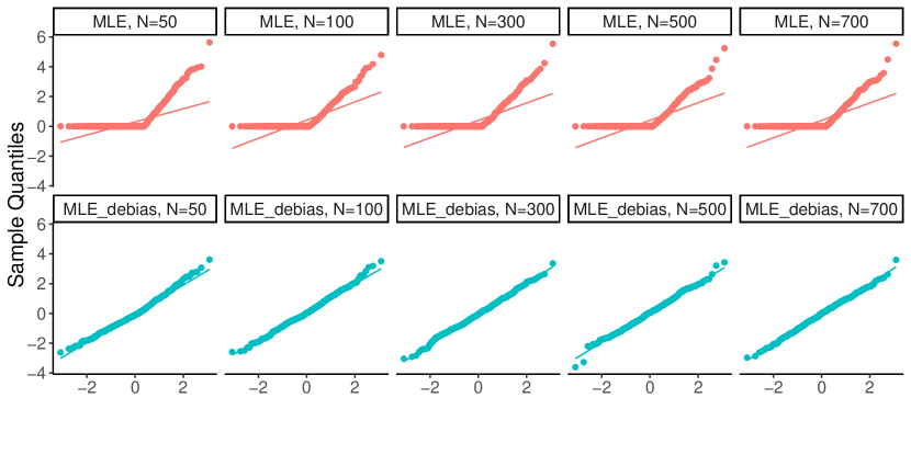
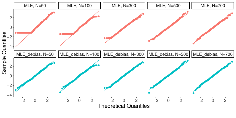
In Section F.2, we also compare the weighted least squares estimator (WLS) in Remark 5 with its counterpart restricted to , and find that WLS converges to normal limits faster than its restricted counterpart.
F.2 Asymptotic normality of the weighted least squares estimator of the mixture weights
We verify the speed of convergence to normal limits of the weighted least squares estimator (WLS) in Remark 5, and compare with its counterpart restricted on (WRLS) given by Eq. 156. We follow the same settings used in Section F.1. As shown in Fig. 3, WLS converges to normal limits at much faster speed than WRLS in both dense and sparse settings.
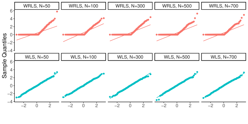
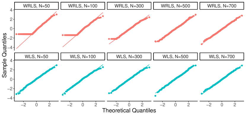
F.3 Impact of weight estimation on distance estimation
In this section, we construct confidence intervals for , based on two possible distance estimators: (i) , the plug-in distance estimator, with weights estimated by the debiased MLE (41) and (43) above; (ii) , the plug-in distance estimator with weights estimated by the weighted least squares estimator given in Remark 5.
We evaluate the coverage and length of 95% confidence intervals (CIs) based on their respective limiting distributions, given in (48) and (154). We illustrate the performance when .
We set , and vary . For each , we generate 10 mixtures for , with each generated according to the dense setting. Then for each , we repeatedly draw 200 pairs of and , sampled from independently, and compute the coverage and averaged length of the 95% CIs for each procedure. For a fair comparison, we assume the two limiting distributions in (48) and (154) known, and approximate their quantiles by their empirical counterparts based on 10,000 realizations. By further averaging the coverages and averaged lengths of 95% CIs over , we see in Table 1 that although both procedures have nominal coverage, CIs based on the debiased MLE are uniformly narrower than those based on the WLS, in line with our discussion in Remark 5. The same experiment is repeated for the sparse setting with from which we draw the same conclusion except that the advantage of using the debiased MLE becomes more visible. Furthermore, the CIs based on the debiased MLE get slightly narrower in the sparse setting whereas those based on the WLS remain the same.
| Coverage | The averaged length of 95% CIs | ||||||||||
|---|---|---|---|---|---|---|---|---|---|---|---|
| Dense | 0.950 | 0.948 | 0.961 | 0.942 | 0.950 | 0.390 | 0.276 | 0.195 | 0.113 | 0.087 | |
| 0.933 | 0.948 | 0.955 | 0.945 | 0.948 | 0.403 | 0.285 | 0.202 | 0.116 | 0.090 | ||
| Sparse | 0.961 | 0.952 | 0.964 | 0.944 | 0.952 | 0.372 | 0.263 | 0.186 | 0.107 | 0.083 | |
| 0.945 | 0.955 | 0.966 | 0.953 | 0.959 | 0.402 | 0.285 | 0.201 | 0.116 | 0.090 | ||
F.4 Confidence intervals of the W-distance
In this section, we evaluate the procedures introduced in Section 5.3 for constructing confidence intervals for for both and . Specifically, we evaluate both the coverage and the length of 95% confidence intervals (CIs) of the true W-distance based on: the -out-of- bootstrap (--BS), the derivative-based bootstrap (Deriv-BS) and the plug-in procedure (Plug-in), detailed in Section 5.3.2. For the -out-of- bootstrap, we follow [57] by setting for some . Suggested by our simulation in Section F.7, we choose . For the two procedures based on bootstrap, we set the number of repeated bootstrap samples as 1000. For fair comparison, we also set for the plug-in procedure (cf. Eq. 50).
Throughout this section, we set , and vary . The simulations of Section F.1 above showed that our de-biased estimator of the mixture weights should be preferred even when the MLE is available (the dense setting). The construction of the data driven CIs for the distance only depends on the mixture weight estimators and their asymptotic normality, and not the nature of the true mixture weights. In the experiments presented below, the mixture weights are generated, without loss of generality, in the dense setting. We observed the same behavior in the sparse setting.
F.4.1 Confidence intervals of the W-distance for
We generate the mixture , and for each choice of , we generate pairs of and , sampled from Multinomial independently. We record in Table 2 the coverage and averaged length of 95% CIs of the W-distance over these 200 repetitions for each procedure. We can see that Plug-in and Deriv-BS have comparable performance with the former being more computationally expensive. On the other hand, --BS only achieves the nominal coverage when is very large. As increases, we observe narrower CIs for all methods.
| Coverage | The averaged length of 95% CIs | |||||||
|---|---|---|---|---|---|---|---|---|
| --BS | 0.865 | 0.905 | 0.935 | 0.945 | 0.153 (0.53) | 0.079 (0.23) | 0.059 (0.18) | 0.036 (0.10) |
| Deriv-BS | 0.94 | 0.93 | 0.945 | 0.95 | 0.194 (0.77) | 0.090 (0.31) | 0.064 (0.21) | 0.037 (0.13) |
| Plug-in | 0.96 | 0.93 | 0.94 | 0.945 | 0.195 (0.68) | 0.089 (0.30) | 0.063 (0.21) | 0.037 (0.11) |
F.4.2 Confidence intervals of the W-distance for
In this section we further compare the three procedures in the previous section for . Holding the mixture components fixed, we generate pairs of and their corresponding . For each pair, as in previous section, we generate 200 pairs of based on for each , and record the coverage and averaged length of 95% CIs for each procedure. By further averaging the coverages and averaged lengths over the 10 pairs of , Table 3 contains the final coverage and averaged length of 95% CIs for each procedure. To save computation, we reduce both and the number of repeated bootstrap samples to . As we can see in Table 3, Plug-in has the nominal coverage in all settings. Deriv-BS has similar performance as Plug-in for but tends to have under-coverage for . On the other hand, --BS is outperformed by both Plug-in and Deriv-BS.
| Coverage | The averaged length of 95% CIs | |||||||
|---|---|---|---|---|---|---|---|---|
| --BS | 0.700 | 0.666 | 0.674 | 0.705 | 0.156 (0.67) | 0.082 (0.33) | 0.062 (0.25) | 0.039 (0.16) |
| Deriv-BS | 0.912 | 0.943 | 0.952 | 0.953 | 0.299 (2.71) | 0.140 (0.95) | 0.100 (0.60) | 0.058 (0.31) |
| Plug-in | 0.946 | 0.950 | 0.952 | 0.951 | 0.304 (2.43) | 0.140 (0.90) | 0.100 (0.57) | 0.058 (0.30) |
F.5 Speed of convergence in distribution of the proposed distance estimator
We focus on the null case, , to show how the speed of convergence of our estimator in Theorem 5 depends on , and . Specifically, we consider (i) , and , (ii) , and and (iii) , and . For each combination of and , we generate 10 mixture distributions for , with each generated according to the dense setting. Then for each , we repeatedly draw 10,000 pairs of and , sampled from independently, and compute our estimator . To evaluate the speed of convergence of , we compute the Kolmogorov-Smirnov (KS) distance, as well as the p-value of the two-sample KS test, between our these estimates of and its limiting distribution. Because the latter is not given in closed form, we mimic the theoretical c.d.f. by a c.d.f. based on draws from it. Finally, both the averaged KS distances and p-values, over , are shown in Table 4. We can see that the speed of convergence of our distance estimator gets faster as increases or decreases, but seems unaffected by the ambient dimension (we note here that the sampling variations across different settings of varying are larger than those of varying and ). In addition, our distance estimator already seems to converge in distribution to the established limit as soon as .
| , | , | , | ||||||||
|---|---|---|---|---|---|---|---|---|---|---|
| KS distances | 1.02 | 0.94 | 0.87 | 0.77 | 0.92 | 0.97 | 0.95 | 0.87 | 1.01 | 0.92 |
| P-values of KS test | 0.34 | 0.39 | 0.50 | 0.58 | 0.46 | 0.36 | 0.37 | 0.47 | 0.29 | 0.48 |
F.6 Details of -out-of- bootstrap and the derivative-based bootstrap
In this section we give details of the -out-of- bootstrap and the derivative-based bootstrap mentioned in Section 5.3.1. For simplicity, we focus on . Let be the total number of bootstrap repetitions and be a given estimator of .
For a given integer and any , let and be the bootstrap samples obtained as
Let be defined in (28) by using as well as and . The latter are obtained from (41) based on and . The -out-of- bootstrap estimates the distribution of by the empirical distribution of with .
The derivative-based bootstrap method on the other hand aims to estimate the limiting distribution in Theorem 5. Specifically, let be some pre-defined estimator of . The derivative-based bootstrap method estimates the distribution of
by the empirical distribution of
Here
uses the estimators and obtained from (41) based on the bootstrap samples
F.7 Selection of for -out-of- bootstrap
In our simulation, we follow [57] by setting for some . To evaluate its performance, consider the null case, , and choose , , and . The number of repetitions of Bootstrap is set to 500 while for each setting we repeat 200 times. The KS distance is used to evaluate the closeness between Bootstrap samples and the limiting distribution. Again, we approximate the theoretical c.d.f. of the limiting distribution based on 20,000 draws from it. Figure 4 shows the KS distances for various choices of and . As we we can see, the result of -out-of- bootstrap gets better as increases. Furthermore, it suggests which gives the best performance over all choices of .
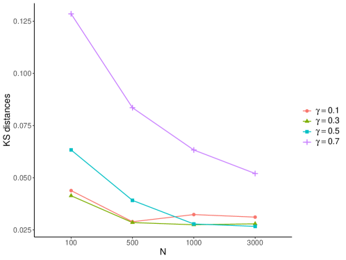
Appendix G Review of the -norm error bound of the MLE-type estimators of the mixture weights in [8]
In this section, we state in details the theoretical guarantees from [8] on the MLE-type estimator in (3) of . Since it suffices to focus on one , we drop the superscripts in this section for simplicity. We assume . Otherwise, a pre-screening procedure could be used to reduce the dimension such that this condition is met.
Recalling from (3) that depends on a given estimator of . Let be a generic estimator of satisfying
| (138) | ||||
| (139) | ||||
| (140) | ||||
| (141) |
for some deterministic sequences , and .111Displays (139) – (141) only need to hold up to a label permutation among columns of .
To state the results in [8], we need a few more notation. For any with , define
The set in conjunction with in (16) are chosen such that
see, for instance, [8, Lemma I.1]. Here is the empirical estimator of . Further define
| (142) |
Recall that (18) and (19). Write
| (143) |
We have . Finally, let
The following results are proved in [8, Theorems 9 & 10].
Theorem 13.
Appendix H Results on the W-distance estimator based on the weighted least squares estimator of the mixture weights
In this section we study the W-distance estimator, in (28), of , by using the weighted least squares estimators
| (147) |
where
| (148) |
with being a generic estimator of . Due to the weighting matrix , is a doubly stochastic matrix, and its largest eigenvalue is (see also Lemma 20, below).
Fix arbitrary . Let
| (149) |
and
| (150) |
with
The following theorem establishes the asymptotic normality of .
Theorem 14.
Proof.
The proof can be found in Section H.1. ∎
Remark 10.
We begin by observing that if is finite, independent of , and is known, the conclusion of the theorem follows trivially from the fact that
and , under no conditions beyond the multinomial sampling scheme assumption. Our theorem generalizes this to the practical situation when is estimated, from a data set that is potentially dependent on that used to construct , and when .
Condition is a mild regularity condition that is needed even if is known, but both and parameters in and are allowed to grow with .
If is rank deficient, so is the asymptotic covariance matrix . This happens, for instance, when the mixture components have disjoint supports and the weight vector is sparse. Nevertheless, a straightforward modification of our analysis leads to the same conclusion, except that the inverse of gets replaced by a generalized inverse and the limiting covariance matrix becomes with and zeroes elsewhere.
The asymptotic normality in Theorem 14 in conjunction with Proposition 1 readily yields the limiting distribution of in (28) by using (147), stated in the following theorem. For arbitrary pair , let
| (152) |
where we assume that the following limit exists
Theorem 15.
Proof.
Consequently, the following corollary provides one concrete instance for which conclusions in Theorem 15 hold for based on in [9].
Corollary 3.
Remark 11 (The weighted restricted least squares estimator of the mixture weights).
We argue here that the WLS estimator in (147) can be viewed as the de-biased estimators of the following restricted weighted least squares estimator
| (156) |
Suppose that and let us drop the superscripts for simplicity. The K.K.T. conditions of (156) imply
| (157) |
Here and are Lagrange variables corresponding to the restricted optimization in (156). We see that the first term on the right-hand side in Eq. 157 is asymptotically normal, while the second one does not always converge to a normal limit. Thus, it is natural to consider a modified estimator
by removing the second term in (157). Interestingly, this new estimator is nothing but in (147). This suggests that converges to a normal limit faster than that of , as confirmed in Figure 2 of Section F.2.
H.1 Proof of Theorem 14
Proof.
For simplicity, let us drop the superscripts. By definition, we have
where we let
| (158) |
with and . Recall that
| (159) |
It suffices to show that, for any ,
| (160) | ||||
| (161) | ||||
| (162) |
Define the condition number of as
| (163) |
Notice that
| (164) |
Proof of Eq. 160: By recognizing that the left-hand-side of (160) can be written as
with , for , being i.i.d. . It is easy to see that and . To apply the Lyapunov central limit theorem, it suffices to verify
This follows by noting that
| by Eq. 159 | ||||
| by Eq. 163 |
and by using and Eq. 164.
Proof of Eq. 161: Fix any . Note that
Further notice that is smaller than
For the first term, since
| (165) |
we obtain
| (166) |
where in the last line we invoke Lemma 20 by observing that condition (171) holds under (151). Section H.1 in conjunction with Section H.2 yields
| (167) |
On the other hand, from Section H.1 and its subsequent arguments, it is straightforward to show
| (168) |
By combining Section H.1 and Section H.1 and by using Eq. 151 together with the fact that
| (169) |
to collect terms, we obtain
Finally, since and Lemma 21 ensures that, for any ,
| (170) |
with probability at least , by also using
we conclude
H.2 Lemmas used in the proof of Theorem 14
The following lemma controls various quantities related with .
Lemma 20.
Proof.
We assume the identity label permutation for Eq. 138 and Eq. 141. First, by using for any symmetric matrix , we find
| (172) |
Then condition (171) guarantees, for any ,
| (173) |
To prove the first result, by Weyl’s inequality, we have
Using again yields
| (174) |
where the step uses and the step is due to . Invoke Eq. 141 to obtain
Together with (172), we conclude . Moreover, we readily see that only requires .
To prove the second result, start with the decomposition
| (175) |
It then follows from dual-norm inequalities, and that
Since, similar to Eq. 172, we also have . Invoke condition Eq. 171 to conclude
completing the proof of the second result.
Finally, Section H.2 and the second result immediately give
The same bound also holds for by the symmetry of and . ∎
Lemma 21.
For any fixed matrix , with probability at least for any , we have
Proof.
Start with and pick any . Note that
By writing
with , we have
To apply the Bernstein inequality, recalling that , we find that has zero mean, for all and
An application of the Bernstein inequality gives, for any ,
Choosing for any and taking the union bounds over yields
with probability exceeding . The result thus follows by noting that
and . ∎