Estimating Galaxy Redshift in Radio-Selected Datasets using Machine Learning
Abstract
All-sky radio surveys are set to revolutionise the field with new discoveries. However, the vast majority of the tens of millions of radio galaxies won’t have the spectroscopic redshift measurements required for a large number of science cases. Here, we evaluate techniques for estimating redshifts of galaxies from a radio-selected survey. Using a radio-selected sample with broadband photometry at infrared and optical wavelengths, we test the -Nearest Neighbours (kNN) and Random Forest machine learning algorithms, testing them both in their regression and classification modes. Further, we test different distance metrics used by the kNN algorithm, including the standard Euclidean distance, the Mahalanobis distance and a learned distance metric for both the regression mode (the Metric Learning for Kernel Regression metric) and the classification mode (the Large Margin Nearest Neighbour metric). We find that all regression-based modes fail on galaxies at a redshift . However, below this range, the kNN algorithm using the Mahalanobis distance metric performs best, with an outlier rate of 5.85%. In the classification mode, the kNN algorithm using the Mahalanobis distance metric also performs best, with an outlier rate of 5.85%, correctly placing 74% of galaxies in the top bin. Finally, we also tested the effect of training in one field and applying the trained algorithm to similar data from another field and found that variation across fields does not result in statistically significant differences in predicted redshifts. Importantly, we find that while we may not be able to predict a continuous value for high-redshift radio sources, we can identify the majority of them using the classification modes of existing techniques.
keywords:
methods: analytical; techniques: photometric; galaxies: photometry; galaxies: high-redshift- 2dfGRS
- 2dF Galaxy Redshift Survey
- AGN
- Active Galactic Nucleus
- ASKAP
- Australian Square Kilometre Array Pathfinder
- ATCA
- Australia Telescope Compact Array
- ATLAS
- Australia Telescope Large Area Survey
- COSMOS
- COSMic evOlution Survey
- DES
- Dark Energy Survey
- DT
- Decision Tree
- eCDFS
- extended Chandra Deep Field South
- ELAIS-S1
- European Large Area ISO Survey–South 1
- EMU
- Evolutionary Map of the Universe
- GP
- Gaussian Process
- kNN
- -Nearest Neighbours
- LMNN
- Large Margin Nearest Neighbour
- LOFAR
- LOw Frequency ARray
- LOTSS
- LOFAR Two-metre Sky Survey
- ML
- Machine Learning
- MLKR
- Metric Learning for Kernel Regression
- MOS
- Multi-Object Spectroscopy
- MSE
- Mean Square Error
- MWA
- Murchison Widefield Array
- NMAD
- Normalised Median Absolute Deviation
- NMI
- Normalised Mutual Information
- OzDES
- Australian Dark Energy Survey
- QSO
- Quasi-Stellar Object
- RF
- Random Forest
- SDSS
- Sloan Digital Sky Survey
- SED
- Spectral Energy Distribution
- SFG
- Star Forming Galaxy
- SKA
- Square Kilometre Array
- SKADS
- Square Kilometre Array Design Survey
- SST
- Spitzer Space Telescope
- SWIRE
- Spitzer Wide-Area Infrared Extragalactic Survey
- WAVES
- Wide Area Vista Extragalactic Survey
1 Introduction
New radio telescopes are set to revolutionise the radio astronomy regime, with the Evolutionary Map of the Universe (EMU) project to be completed on the Australian Square Kilometre Array Pathfinder [ASKAP; Johnston et al., 2007, 2008] telescope in particular set to increase the number of known radio sources from 2.5 million [Norris, 2017] to 70 million [Norris et al., 2011].
For most aspects of science, knowledge of an astronomical source’s redshift is an essential indicator of the distance and age of the source. Ideally, this redshift is measured directly using spectroscopy. However, even with modern advances — including Multi-Object Spectroscopy (MOS) which can allow hundreds to thousands of redshifts to be measured at once — deep spectroscopic surveys still fail to yield reliable redshifts from 30-60% of measured spectra [Newman et al., 2015]. Currently, the Sloan Digital Sky Survey (SDSS) has measured 4.8 million spectroscopic redshifts — as of the 16th data release [Ahumada et al., 2020]111https://www.sdss.org/dr16/scope/ — and the 2dF Galaxy Redshift Survey [2dfGRS; Lewis et al., 2002] measured 250 000 spectroscopic redshifts over its 5 year project222http://www.2dfgrs.net/Public/Survey/statusfinal.html. In the future, the Wide Area Vista Extragalactic Survey (WAVES) survey — expected to provide a further 2.5 million spectroscopic redshift measurements [Driver et al., 2016] — will increase the number of spectroscopically measured sources. However, this will still be significantly short of the expected million sources detected by the EMU project (even if all of these newly measured galaxies were exclusively selected from the EMU survey).
Photometric template fitting [Baum, 1957] is able to estimate the redshift (hereafter ) of a source, as well as ancillary data like galaxy classification. Photometric template fitting is completed by comparing the Spectral Energy Distribution (SED), measured across as many different wavelengths as possible, to templates constructed with astrophysical knowledge, or prior examples. Figure 1 shows the 31 filter bands available in the COSMic evOlution Survey (COSMOS) field and an example SED used by Ilbert et al. [2009] to achieve redshift accuracies of .

Machine Learning (ML) has also been applied to the problem, with the kNN algorithm [Ball et al., 2007, 2008, Oyaizu et al., 2008, Zhang et al., 2013, Kügler et al., 2015, Cavuoti et al., 2017, Luken et al., 2019, 2021], Random Forest [RF; Cavuoti et al., 2012, 2015, Hoyle, 2016, Sadeh et al., 2016, Cavuoti et al., 2017, Pasquet-Itam and Pasquet, 2018], and neural networks [Firth et al., 2003, Tagliaferri et al., 2003, Collister and Lahav, 2004, Brodwin et al., 2006, Oyaizu et al., 2008, Hoyle, 2016, Sadeh et al., 2016, Curran, 2020, Curran et al., 2021] being among the more widely used algorithms. Some recent studies utilise Gaussian Process [GP; Duncan et al., 2018a, b, 2021], and deep learning using the original images at different wavelengths, as opposed to the photometry extracted from the image [D’Isanto and Polsterer, 2018].
However, few of these solutions are appropriate for the large-scale radio surveys being conducted. While photometric template fitting provides a theoretically ideal solution, the quality of data required to make it highly accurate will not be available for the majority of sources in the all-sky EMU survey, since only all-sky photometric data will be available for most sources. An example of the broadband photometry used by this work is shown in Figure 2, which shows both a likely Active Galactic Nucleus (AGN; top), and Star Forming Galaxy (SFG; bottom).
Additionally, Norris et al. [2019] has shown that photometric template fitting performs poorly on radio-selected data sets (which are typically dominated by Active Galactic Nucleus (AGN)), possibly because the majority of templates are unable to differentiate between emission from the AGN and emission from the galaxy itself [Salvato et al., 2018].

The ML based methods have mainly focused on optically-selected datasets, with most work drawing on the SDSS photometric and spectroscopic samples, often restricting the redshift range to , or using datasets containing only one type of object — e.g. the SDSS Galaxy or Quasi-Stellar Object (QSO) catalogs. While this kind of testing is entirely appropriate for non-radio selected samples, Norris et al. [2019] have shown that assumptions in the optical regime may not be valid in the radio regime, for two reasons. First, the redshift distribution of radio-selected sources is quite different from that of optically-selected sources, as shown in Figure 3. Second, radio-selected sources are often dominated by a radio-loud AGN which is poorly represented in optically-selected templates and training sets.
Finally, we should note that in support of the science goals of the EMU Project, we aim to minimise the number of estimations that catastrophically fail, rather than minimise for accuracy as most other works do.

The overall contributions of this study include:
-
1.
An in-depth study of the simple -Nearest Neighbours algorithm, including the investigation of typically ignored distance metrics for the estimation of radio galaxy redshift;
-
2.
A comparison with the widely used Random Forest algorithm;
-
3.
An analysis of whether similarly observed fields can be used as training samples for alternate fields;
-
4.
An exploration into the effectiveness of regression vs classification modes in estimating high redshift galaxies, given the highly unbalanced nature of the training sample (noting that while classification modes might be able to identify high-redshift galaxies, it will not be able to estimate its actual redshift).
1.1 Formal Problem Statement
In this article, we investigate the problem of modelling the redshift of a source with respect to known measurements of the source. This can be a regression problem, where we attempt to model the function , such that the redshift of source , and the known measurements of source are obtained from a catalogue with various domains. We can also model the redshift of a source as , where is a class representing a specific domain of redshift. In the following section we describe the catalogues containing the known source information and the variables that are used for this representation.
2 Data
This work uses data from the Australia Telescope Large Area Survey [ATLAS; Norris et al., 2006, Franzen et al., 2015] radio continuum catalogue, providing a 1.4 GHz flux density measurement of 4780 unique sources. The Australia Telescope Large Area Survey (ATLAS) survey covers two regions of the sky – the extended Chandra Deep Field South (eCDFS) and the European Large Area ISO Survey–South 1 (ELAIS-S1), both to a depth of , and was completed as a first-look at what the EMU survey may provide. This survey was cross-matched by Swan [2018] with the Australian Dark Energy Survey [OzDES; Yuan et al., 2015, Childress et al., 2017, Lidman et al., 2020], Dark Energy Survey [DES; Dark Energy Survey Collaboration et al., 2016] and Spitzer Wide-Area Infrared Extragalactic Survey [SWIRE; Lonsdale et al., 2003] surveys, providing spectroscopic redshift measurements, g, r, i and z optical magnitudes, and 3.6, 4.5, 5.4 and 8.0 m infrared flux measurements respectively.
This work used only those ATLAS sources with measured photometry in all provided optical and infrared bands, creating a final dataset containing 1311 sources with complete photometric coverage. Specifically, in both fields used in this work, we used the g, r, i and z optical magnitudes from Dark Energy Survey (DES), and 3.6, 4.5, 5.4 and 8.0 m infrared flux measurements from the Spitzer Wide-Area Infrared Extragalactic Survey (SWIRE) survey, as shown in Figure 4. The redshift distribution of the final collated dataset is presented in Figure 5.


To prevent the different methods tested from being dominated by single features with wide variation, all features were standardised using Equation 1, setting the feature mean to 0, and the feature variance to unit variance.
| (1) |
where is the mean of the sample of variable and is its standard deviation.
During testing, we also examined the use of “colours” rather than optical magnitudes, and taking the log of the radio and infrared fluxes to better distribute the data. Colours are typically used instead of magnitudes to remove the brightness- and redshift-dependent nature of magnitudes, replacing them by the difference between the magnitudes that is dependent only on the SED.
2.1 Data Partitioning
All machine learning methods require the main dataset to be partitioned into multiple subsets, with the subsets set aside for training the model, validating hyperparameters, and testing the model. In this work, we split our data into two datasets – training and testing, with the hyper-parameters being validated using -fold cross validation on the training set. We partition our data differently for the three tests we complete:
-
1.
Typical random split, with 70% of the data split off as the training set, leaving the remaining 30% as the test set.
- 2.
- 3.
In addition to the above partitioning, in order to facilitate the use of the classification modes of our algorithms tested, we quantise the redshift values into 15 redshift bins (defined in Table 1), with equal numbers of sources in each in order to be able to predict a uniform distribution with using a matching distribution. The median of the spectroscopic redshifts within the bin is chosen as the redshift to predict.
| Bin | Lower | Upper | Median |
|---|---|---|---|
| Number | Bound | Bound | Value |
| 1 | 0 | 0.10 | |
| 2 | 0.10 | 0.15 | 0.12 |
| 3 | 0.15 | 0.19 | 0.17 |
| 4 | 0.19 | 0.22 | 0.21 |
| 5 | 0.22 | 0.26 | 0.24 |
| 6 | 0.26 | 0.29 | 0.27 |
| 7 | 0.29 | 0.32 | 0.31 |
| 8 | 0.32 | 0.35 | 0.34 |
| 9 | 0.35 | 0.41 | 0.38 |
| 10 | 0.41 | 0.50 | 0.46 |
| 11 | 0.50 | 0.58 | 0.54 |
| 12 | 0.58 | 0.66 | 0.62 |
| 13 | 0.66 | 0.80 | 0.73 |
| 14 | 0.80 | 1.02 | 0.91 |
| 15 | 1.02 | 4.33 |
3 Methods
3.1 kNN
The kNN algorithm [Cover and Hart, 1967] computes a similarity matrix between all sources based on the catalogue’s photometric measurements, and a given distance metric (the set of distance metrics tested in this work are explained in Subsections 3.1.1, 3.1.2, and 3.1.3). Once the similarity matrix is constructed, the kNN algorithm finds the (Hereafter ) most similar sources with measured redshifts (where is optimised using cross validation), and takes either the mean value (for regression) or the mode class (for classification) of the sources as the estimated redshift for each source. A simple illustration of the kNN algorithm is shown in Figure 6

The value of used in the kNN in this work is optimised using -fold (where is hereafter and is set to 10 for this work) cross-validation. -fold cross-validation randomly splits the data into roughly even groups, iterating through using groups as the training set and validating on the remaining group, until every group has been used in testing, with the average error used as the error for that value of . This work tested all integer values of for the kNN algorithm between 2 and 20 ().
The kNN algorithm requires a metric to determine which of the observations are neighbours to a given observation. In the next sections we present the set of metrics investigated in the experiment.
3.1.1 Euclidean Distance
Euclidean Distance is the simplest, and most widely used distance metric in literature, defined in Equation 2:
| (2) |
where is the Euclidean distance between two feature vectors and . In this case the vectors contain the measured photometry of two galaxies.
3.1.2 Mahalanobis Distance
The Mahalanobis distance metric [Mahalanobis, 1936] normalises the variance and covariance of the input features by transforming the features using the inverse of the covariance matrix. For uncorrelated input features, the Mahalanobis distance is equal to the scaled Euclidean distance, but for correlated features, it generalises the idea of Euclidean distance to take account of the covariance. The Mahalanobis distance is defined in Equation 3:
| (3) |
where is the Mahalanobis distance between two feature vectors and , and is the covariance matrix.
3.1.3 Learned Distance Metrics
Conceptually, for best results the distance metric used should take into consideration the shape and structure of the data. Towards this end, we can generalise Equations 2, and 3 to Equation 4, noting that the matrix can be any positive semi-definite matrix. The Identity matrix is used for Euclidean Distance, and the matrix is used in the Mahalanobis. We can, however, go one step further, and attempt to learn an matrix that can better warp the feature space so that observations with similar redshift are measured as close, while observations with different redshift are measured as distant.
| (4) |
where is the distance between two feature vectors and .
For our regression tests, we used the Metric Learning for Kernel Regression (MLKR) distance metric, which performs a supervised Principle Component Analysis [Weinberger and Tesauro, 2007]. The MLKR distance metric begins by decomposing the matrix from Equation 4 using Equation 5:
| (5) |
Using Equation 5, Equation 4 can be expressed as the modified Euclidean Distance metric in Equation 6:
| (6) |
Matrix is optimised using Gradient Descent, using Equation 7:
| (8) |
| (9) |
The loss function being minimised is a simple squared difference, defined in Equation 10:
| (10) |
For our Classification tests, the Large Margin Nearest Neighbour [LMNN; Weinberger et al., 2006] learned distance metric was used. The Large Margin Nearest Neighbour (LMNN) distance metric finds a transformation for the data that maximises the distance between different classes, and minimises the distance between similar classes. The loss function the LMNN algorithm optimises is defined in Equation 11:
| (11) |
where , , and are individual galaxy feature vectors, describes whether is a target of , is a positive constant typically chosen through cross-validation and – a hinge function.
An example of the transformation the LMNN algorithm attempts is in Figure 7, using three neighbours.

3.2 Random Forest
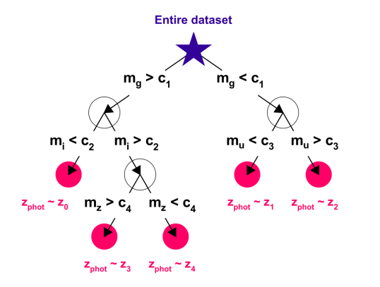
For comparison, we have contrasted our results with the popular and well-used Random Forest (RF) algorithm. RFs are constructed from bootstrapped Decision Trees – an algorithm that partitions the data space so that it can be explored using a tree, shown in Figure 8 [Morgan and Sonquist, 1963, Quinlan, 1987]. Each DT finds the impurity at each node (defined in Equation 12) to determine the best features and values to split the data on:
| (12) |
where is the data at node , is a subset of data, is the number of objects at node , and are the numbers of objects on the left and right sides of the split, and are the objects on the left and right sides of the split, and the function is a impurity function that differs between classification and regression. For Regression, the Mean Square Error is used (defined in Equation 13), whereas Classification often uses the Gini Impurity (defined in Equation 14).
| (13) |
where is the number of objects at node and and are the response variables.
| (14) |
where is the proportion of split that are class , defined formally in Equation 15:
| (15) |
where is the indicator function, identifying the correct classifications.
3.3 Error Metrics
In order to evaluate each of the machine learning models, the prediction error of each model will be assessed. In this section, the set of statistics that measure the error of the models are presented. The primary error metric compared in this work is the outlier rate, defined in Equation 16:
| (16) |
where . The outlier rate is a percentage representing the number of ‘catastrophic failures’ (the percentage of galaxies that have a residual greater than 0.15, scaled with redshift), and is commonly found in literature [Ilbert et al., 2009, Salvato et al., 2009, 2011, Cavuoti et al., 2012, Zitlau et al., 2016, Cavuoti et al., 2017, Jones and Singal, 2017, Mountrichas et al., 2017, Luken et al., 2019, Norris et al., 2019].
We also provide a secondary outlier rate in order to provide a statistically sound comparison, defined in Equation 17:
| (17) |
where , and is the standard deviation of the estimated response, defined in Equation 18:
| (18) |
where is the number of observations, is an observation, and is the estimated observation.
As this work is presenting both regression and classification modes of the given algorithms, there are some error metrics that suit regression, and some that suit classification. These metrics are defined in Subsection 3.3.1 and 3.3.2 respectively.
3.3.1 Regression Error Metrics
For the regression tests, three additional error metrics were compared. The first is the Normalised Median Absolute Deviation (NMAD). The NMAD is a similar measure to the standard deviation, and is generally used for non-Gaussian distributions. It is more robust than the standard deviation, as it takes the median of the residuals, improving the resilience to outliers – an issue that can be prominent in redshift estimation due to the highly unbalanced data sets used, and is defined in Equation 19:
| (19) |
where is the Normalised Median Absolute Deviation, is a vector of residuals from which is taken.
The Coefficient of Determination is the second regression-based error metric, and is the proportion of variance explained by the model, The is defined in Equation 20:
| (20) |
where is a response variable, is the corresponding estimated response, and is the mean of the response variables.
Finally, the Mean Square Error (MSE) is a direct measure of the error produced by the model, with the lower the value the better, and is defined in Equation 21:
| (21) |
where is the number of observations, is the measured response, and is the estimated response.
3.3.2 Classification Error Metrics
Traditionally in ML classification settings, the Accuracy (defined in Equation 22), Precision, Recall and F1 score are reported. We also investigated the Normalised Mutual Information, which suggests how dependent one set of data is upon another. We do not report the Precision, Recall, F1 Score and Normalised Mutual Information, however, as we found they provided no additional information.
It is important to note that the main error metric being compared and minimised in both the regression and classification tests is the outlier rate. As this outlier rate is explicitly accepting of a level of inaccuracy that scales with redshift, there is an inherent acceptance of some level of leakage between neighbouring classes during classification tests.
This acceptance of leakage means that models may present with high error rates due to rigid correct/incorrect classifications, and yet may still be acceptable models for this process.
| (22) |
where is the measured response, is the predicted response, is the number of samples, and is an indicator function, indicating the cases where the predicted response matched the measured response.
3.4 Statistical Significance
Analysis of Variance (ANOVA) tests were used in this study to test for statistical significance. This allows us to test whether the changes in model correlate to a statistically significant change in estimated redshift, by testing to see if the means of two or more populations (in this case, experiments with different models) differ.
In all cases, the tests were run in a one-vs-many scenario, with the one being tested as our best performing metric in order to determine whether our best performing result is statistically significant.
3.5 Software
This work makes use of the Scikit-learn333https://scikit-learn.org/ Python package [Pedregosa et al., 2011] for the implementation of the RF and kNN algorithms, as well as the Euclidean and Mahalanobis distance metrics. We made use of the PyLMNN444https://pypi.org/project/PyLMNN/ package for the LMNN distance metric, and the metric-learn555http://contrib.scikit-learn.org/metric-learn/generated/metric_learn.MLKR.html package for the MLKR distance metric. The code and data used in this work is available on Github666https://github.com/kluken/Redshift-kNN-2021.
4 Results
Given the number of different algorithms, distance metrics and datasets tested in this work, we have assigned each combination a Test ID, defined in Table 2 for Regression-based tests, and Table 3 for Classification-based tests. Each test ID is made up of 4 characters, with the first character (R/C) representing whether the test is a regression- or classification-based test, the 2nd and 3rd characters (Eu/Ma/ML/Rf) representing the method used for estimation (Euclidean distance, Malanobis distance, a Learned distance metric, or Random Forest), and the final character (1/2/3) representing the training set used (1 = Random, 2 = ELAIS-S1, 3 = eCDFS).
As discussed in Section 2, we tested both statistical standardisation of input photometry, compared with the use of astrophysically derived “colours”, and taking the log of radio and infrared data to better distribute the data. In both cases, however, the result was very similar to the standardised dataset, and hence is the only value quoted.
| Test ID | Method | Distance Metric | Training Set |
| REu1 | kNN | Euclidean | Random |
| REu2 | kNN | Euclidean | ELAIS-S1 |
| REu3 | kNN | Euclidean | eCDFS |
| RMa1 | kNN | Mahalanobis | Random |
| RMa2 | kNN | Mahalanobis | ELAIS-S1 |
| RMa3 | kNN | Mahalanobis | eCDFS |
| RML1 | kNN | MLKR | Random |
| RML2 | kNN | MLKR | ELAIS-S1 |
| RML3 | kNN | MLKR | eCDFS |
| RRf1 | RF | – | Random |
| RRf2 | RF | – | ELAIS-S1 |
| RRf3 | RF | – | eCDFS |
| Test ID | Method | Distance Metric | Training Set |
| CEu1 | kNN | Euclidean | Random |
| CEu2 | kNN | Euclidean | ELAIS-S1 |
| CEu3 | kNN | Euclidean | eCDFS |
| CMa1 | kNN | Mahalanobis | Random |
| CMa2 | kNN | Mahalanobis | ELAIS-S1 |
| CMa3 | kNN | Mahalanobis | eCDFS |
| CML1 | kNN | LMNN | Random |
| CML2 | kNN | LMNN | ELAIS-S1 |
| CML3 | kNN | LMNN | eCDFS |
| CRf1 | RF | – | Random |
| CRf2 | RF | – | ELAIS-S1 |
| CRf3 | RF | – | eCDFS |
4.1 Regression
Based on the Regression tests outlined in Table 2, we present the results in a series of plots (Figures 9, 10, 11, and 12).
In each plot three subfigures are presented, with Subfigure A representing the random training set, Subfigure B representing the training set built using galaxies from the ELAIS-S1 field, and Subfigure C representing the training set built using galaxies from the eCDFS field. The subfigures are split into two plots – the top plot showing the measured spectroscopic redshift (x-axis) compared with the predicted redshift (y-axis), with a perfect 1:1 correlation (red dashed line) and the outlier rate boundaries (blue dashed lines) shown. The bottom plot shows the measured spectroscopic redshift (x-axis) against the residuals, again with the perfect 1:1 correlation (red dashed line) and the outlier rate boundaries (blue dashed lines) shown.
These results are summarised in Table 4.
| Test | / | MSE | |||||
|---|---|---|---|---|---|---|---|
| Trees | (%) | (%) | Value | ||||
| REu1 | 5 | 8.14 | 6.61 | 0.65 | 0.06 | 0.10 | 0.05 |
| REu2 | 5 | 8.70 | 5.51 | 0.60 | 0.06 | 0.12 | 0.06 |
| REu3 | 11 | 8.28 | 4.85 | 0.53 | 0.09 | 0.12 | 0.06 |
| RMa1 | 5 | 5.85 | 5.09 | 0.59 | 0.07 | 0.12 | 0.03 |
| RMa2 | 3 | 8.70 | 5.39 | 0.58 | 0.07 | 0.15 | 0.04 |
| RMa3 | 5 | 7.68 | 5.45 | 0.54 | 0.09 | 0.13 | 0.04 |
| RML1 | 4 | 6.36 | 4.07 | 0.73 | 0.05 | 0.10 | 0.05 |
| RML2 | 9 | 8.58 | 4.78 | 0.68 | 0.05 | 0.11 | 0.06 |
| RML3 | 5 | 10.91 | 4.44 | 0.58 | 0.08 | 0.13 | 0.05 |
| RRf1 | 44 | 8.14 | 4.84 | 0.59 | 0.07 | 0.13 | 0.05 |
| RRf2 | 21 | 12.75 | 5.88 | 0.32 | 0.11 | 0.19 | 0.06 |
| RRf3 | 23 | 10.71 | 4.65 | 0.54 | 0.09 | 0.14 | 0.06 |


We show that the lowest outlier rate is achieved using the kNN algorithm paired with the Mahalanobis distance metric, and is statistically different from most other algorithms (kNN using Euclidean Distance: p value = 0.0183, and the RF algorithm: p value = 0.0183 compared with kNN using the Mahalanobis distance metric as a baseline). The kNN algorithm using the MLKR distance metric (a Mahalanobis-like distance metric) is not statistically significantly different (p value = 0.5750). However, all results (including the RF algorithm) suffer from the same issues of under-predicting high redshift () galaxies.
The randomly selected training sets typically achieve lower outlier rates than the training sets built using one field only, however, neither field-based training set provides consistently better outlier rates than the other. This is confirmed statistically, with no statistically significant result measured (p value = 0.2072).
4.2 Classification
Based on the Classification tests outlined in Table 3, we show the classification-based results for the kNN algorithm – using Euclidean distance (Figure 14), Mahalanobis distance (Figure 15) and the LMNN learned distance metric (Figure 16) – and the RF algorithm (Figure 17), summarised in Table 5.
We present our classification-based results using scaled confusion matrices, where the x-axis shows the measured spectroscopic redshift, the y-axis shows the predicted redshift, the colour shows the density of the objects in that chosen bin, and the width of each bin is proportional to the range of redshift values represented by the bin. An example scatter plot (in the same style as Figure 9), demonstrating the effect of binning on the classification results when compared against the original spectroscopic measurements is shown in Figure 13.

| Test | / | Acc | |||
|---|---|---|---|---|---|
| Trees | (%) | (%) | |||
| CEu1 | 6 | 8.91 | 4.07 | 0.30 | 0.10 |
| CEu2 | 5 | 12.13 | 3.55 | 0.24 | 0.14 |
| CEu3 | 8 | 11.31 | 5.05 | 0.27 | 0.13 |
| CMa1 | 11 | 5.85 | 3.57 | 0.50 | 0.14 |
| CMa2 | 6 | 7.60 | 4.41 | 0.37 | 0.14 |
| CMa3 | 13 | 7.88 | 3.43 | 0.40 | 0.13 |
| CML1 | 7 | 6.36 | 5.85 | 0.40 | 0.09 |
| CML2 | 8 | 9.93 | 4.04 | 0.32 | 0.16 |
| CML3 | 7 | 9.90 | 4.04 | 0.40 | 0.13 |
| CRf1 | 53 | 7.12 | 3.82 | 0.36 | 0.10 |
| CRf2 | 39 | 10.54 | 4.41 | 0.27 | 0.14 |
| CRf3 | 32 | 10.91 | 4.24 | 0.33 | 0.15 |
The kNN algorithm paired with the Mahalanobis distance metric provides the lowest and outlier rates, as well as performing the best in terms of traditional ML classification metrics (accuracy, precision, recall and F1 score). However, while the results using the Mahalanobis distance metric are statistically significantly better than those using the Euclidean distance metric (p = 0.00619), they are not statistically different from the LMNN learned distance metric (a Mahalanobis-like distance metric; p = 0.4276), or the RF algorithm (p = 0.8913). Again, we note that for most algorithms, the highest redshift galaxies remain a problem for estimation, however, the results can change significantly based on the distance metric used – for example, the bin was correctly predicted 50% of the time using the kNN algorithm paired with Euclidean distance, however, using the Mahalanobis distance metric brought this up to 74%.
As with the regression tests, the random training sample outperformed the training sets built from a single field in the primary error metric, however, the results are statistically insignificant (p = 0.4397).


5 Discussion
Most previous work has treated the estimation of galaxy redshift as a regression task – estimating a continuous value for redshift. We have shown that the kNN algorithm – when using either a learned distance metric, or the Mahalanobis distance metric – outperforms the RF algorithm, particularly at a redshift of . At a redshift of , both the kNN and RF have systematic under-estimations, likely caused by the unbalanced training sample used, with the vast majority of samples at lower redshifts.
Here we try a different approach, by treating the problem of calculating point estimates of redshifts as a classification problem. Previous works have calculated probability density functions (PDFs) for galaxies by finely binning data and treating it as a classification problem [Gerdes et al., 2010, Pasquet-Itam and Pasquet, 2018, Eriksen et al., 2020]. However, this is subtly different to this work as the primary purpose here is to identify the high-redshift galaxies – not to generate PDFs. We balance the data by binning the data into 15 bins with equal numbers of sources. By allowing this coarse mapping, we ensure that all redshift values we are attempting to predict are equally represented, and can therefore obtain better results at the higher redshift ranges. In particular, we have included a bin, which in our best results (the kNN algorithm using the Mahalanobis distance metric) we predict in 74% of cases (85% of galaxies at predicted in the highest two bins). Again, the kNN algorithm is able to outperform the RF algorithm.
In addition to the regression and classification tests, we tested using different training samples. The first training sample is made up of a random selection across both the ELAIS-S1 and eCDFS fields. The second and third samples were made up of only one of the fields, which was then used to predict the other. As expected, the random sample modelled the test sets better – though not significantly – than the training samples taken from a single field only. This is likely due to observational differences – while the surveys used in this work were designed to be as homogeneous as possible, there will always be slight differences.
One such difference is the number of sources in each field. While there is not expected to be differences in the actual source counts between these fields, there is the potential issue of minor observational issues (for example, in the radio regime, there may have been more radio-frequency interference in one set of observations than another. In the optical regimes, it may have been that there was slightly different sky conditions affecting the observations) affecting the fields differently.
5.1 Comparison with Previous Works
Fair comparisons with previous works are often difficult due to different features being selected — often studies are conducted on well-observed, feature rich fields like the COSMOS field, providing a wealth of UV, NIR and X-ray data that is typically not available for the majority of the sky — and different selection methods — selecting sources from the SDSS Galaxy survey, where the redshift range is restricted towards higher redshift and typically don’t have a radio-counterpart, which are shown by Norris et al. [2019] to be a more difficult challenge. Where the data sets have been AGN selected, using similar features as in Duncan et al. [2021, Lockman Hole AGN Experiments], we find our results are highly competitive, providing a lower outlier rate ( compared with , albeit with a higher scatter ( compared with ), suggesting that while we are less accurate than others, we are having fewer estimates catastrophically fail. This optimisation of outlier rate (reducing the number of estimations that catastrophically fail) is motivated by the science goals of the EMU Project. We note that this comparison should be further tempered by the fact that the differing training and test set sizes, and the redshift distribution of the overall datasets have a large impact on the overall statistics.

6 Conclusion
We have used a radio-selected point-source catalogue consisting of ATLAS radio data, DES optical photometry, SWIRE infrared data and OzDES spectroscopic redshifts to test the kNN and RF algorithms for estimating the redshift of galaxies.
We have used both regression and classification modes of these algorithms in order to balance highly unbalanced training sets, and have shown that using classification modes increases the effectiveness of the algorithms at a redshift of (noting that while we are generally able to identify the galaxies at , we are unable to estimate their exact redshift). Given this increase in effectiveness at isolating the high-redshift galaxies using classification methods, a mix of classification- and regression-based methods would provide the best possible result over larger redshift ranges, allowing the higher redshift galaxies to be identified, while still being able to estimate the redshift of nearby galaxies to high accuracy.
In our tests we have shown that when using the classification modes of the algorithms, the kNN algorithm using the Mahalanobis distance metric performs better than the alternative methods tested. We particularly note that the bin was correctly predicted in 74% of cases – far better than the regression regimes that fail consistently at that range.
When using the regression modes of the algorithms, the kNN algorithm using the Mahalanobis distance metric performed statistically significantly better than most of the alternate methods tested (kNN using Euclidean Distance: p value = 0.0183, and the RF algorithm 0.0183) – the kNN algorithm paired with the Mahalanobis-like MLKR distance metric was statistically insignificantly different (p = 0.5750). In both regression and classification methods, the kNN algorithm outperforms the much more widely used RF algorithm.
Finally, we tested whether there would be a significant difference in the outlier rate between a model trained and tested on randomly split data, and a model that is trained on one field of sky and tested on another. While the results were generally suggestive of the random training sample out-performing the field-specific training samples, the difference is not statistically significant (Regression p value = 0.2072 and classification p value = 0.4397). This suggests that for new fields being observed with similar strategies to previously observed fields, any differences in measured photometry should produce minimal effect on the estimated redshifts. It should be noted, however, that this does not take into consideration any differences in photometry caused by differences in telescopes. For example, if a galaxy was to have SkyMapper , , and photometry instead of DES photometry. To determine the impact of changes of telescopes on the data would require further testing, and will be the subject of further work utilising Transfer Learning.
7 Implications for Future Radio Surveys
Traditional photometric template fitting methods typically struggle to estimate the redshift of radio galaxies. In the near future, large area radio surveys like the EMU survey are set to revolutionise the field of Radio Astronomy, with the number of known radio galaxies set to increase by an order of magnitude. This work shows that broadband photometry at similar wavelengths to those available in present and near-complete all-sky surveys will be enough to estimate acceptable redshifts for 95% of radio sources with coverage over those bands. Further, while continuous redshift values are particularly difficult to estimate for radio sources at high-redshift, they can still be identified as high redshift with the majority of sources correctly placed in the highest redshift bin using classification modes.
Acknowledgments
The Australia Telescope Compact Array is part of the Australia Telescope National Facility which is funded by the Australian Government for operation as a National Facility managed by CSIRO. We acknowledge the Gomeroi people as the traditional owners of the Observatory site.
Based in part on data acquired at the Anglo-Australian Telescope. We acknowledge the traditional owners of the land on which the AAT stands, the Gamilaroi people, and pay our respects to elders past and present.
This project used public archival data from the Dark Energy Survey (DES). Funding for the DES Projects has been provided by the U.S. Department of Energy, the U.S. National Science Foundation, the Ministry of Science and Education of Spain, the Science and Technology FacilitiesCouncil of the United Kingdom, the Higher Education Funding Council for England, the National Center for Supercomputing Applications at the University of Illinois at Urbana-Champaign, the Kavli Institute of Cosmological Physics at the University of Chicago, the Center for Cosmology and Astro-Particle Physics at the Ohio State University, the Mitchell Institute for Fundamental Physics and Astronomy at Texas A&M University, Financiadora de Estudos e Projetos, Fundação Carlos Chagas Filho de Amparo à Pesquisa do Estado do Rio de Janeiro, Conselho Nacional de Desenvolvimento Científico e Tecnológico and the Ministério da Ciência, Tecnologia e Inovação, the Deutsche Forschungsgemeinschaft, and the Collaborating Institutions in the Dark Energy Survey.
The Collaborating Institutions are Argonne National Laboratory, the University of California at Santa Cruz, the University of Cambridge, Centro de Investigaciones Energéticas, Medioambientales y Tecnológicas-Madrid, the University of Chicago, University College London, the DES-Brazil Consortium, the University of Edinburgh, the Eidgenössische Technische Hochschule (ETH) Zürich, Fermi National Accelerator Laboratory, the University of Illinois at Urbana-Champaign, the Institut de Ciències de l’Espai (IEEC/CSIC), the Institut de Física d’Altes Energies, Lawrence Berkeley National Laboratory, the Ludwig-Maximilians Universität München and the associated Excellence Cluster Universe, the University of Michigan, the National Optical Astronomy Observatory, the University of Nottingham, The Ohio State University, the OzDES Membership Consortium, the University of Pennsylvania, the University of Portsmouth, SLAC National Accelerator Laboratory, Stanford University, the University of Sussex, and Texas A&M University.
Based in part on observations at Cerro Tololo Inter-American Observatory, National Optical Astronomy Observatory, which is operated by the Association of Universities for Research in Astronomy (AURA) under a cooperative agreement with the National Science Foundation.
This work is based on archival data obtained with the Spitzer Space Telescope, which was operated by the Jet Propulsion Laboratory, California Institute of Technology under a contract with NASA. Support for this work was provided by an award issued by JPL/Caltech
References
- Ahumada et al. [2020] Ahumada, R., Prieto, C.A., Almeida, A., Anders, F., Anderson, S.F., Andrews, B.H., Anguiano, B., Arcodia, R., Armengaud, E., Aubert, M., Avila, S., Avila-Reese, V., Badenes, C., Balland, C., Barger, K., Barrera-Ballesteros, J.K., Basu, S., Bautista, J., Beaton, R.L., Beers, T.C., Benavides, B.I.T., Bender, C.F., Bernardi, M., Bershady, M., Beutler, F., Bidin, C.M., Bird, J., Bizyaev, D., Blanc, G.A., Blanton, M.R., Boquien, M., Borissova, J., Bovy, J., Brandt, W.N., Brinkmann, J., Brownstein, J.R., Bundy, K., Bureau, M., Burgasser, A., Burtin, E., Cano-Díaz, M., Capasso, R., Cappellari, M., Carrera, R., Chabanier, S., Chaplin, W., Chapman, M., Cherinka, B., Chiappini, C., Doohyun Choi, P., Chojnowski, S.D., Chung, H., Clerc, N., Coffey, D., Comerford, J.M., Comparat, J., da Costa, L., Cousinou, M.C., Covey, K., Crane, J.D., Cunha, K., Ilha, G.d.S., Dai, Y.S., Damsted, S.B., Darling, J., Davidson, James W., J., Davies, R., Dawson, K., De, N., de la Macorra, A., De Lee, N., Queiroz, A.B.d.A., Deconto Machado, A., de la Torre, S., Dell’Agli, F., du Mas des Bourboux, H., Diamond-Stanic, A.M., Dillon, S., Donor, J., Drory, N., Duckworth, C., Dwelly, T., Ebelke, G., Eftekharzadeh, S., Davis Eigenbrot, A., Elsworth, Y.P., Eracleous, M., Erfanianfar, G., Escoffier, S., Fan, X., Farr, E., Fernández-Trincado, J.G., Feuillet, D., Finoguenov, A., Fofie, P., Fraser-McKelvie, A., Frinchaboy, P.M., Fromenteau, S., Fu, H., Galbany, L., Garcia, R.A., García-Hernández, D.A., Oehmichen, L.A.G., Ge, J., Maia, M.A.G., Geisler, D., Gelfand, J., Goddy, J., Gonzalez-Perez, V., Grabowski, K., Green, P., Grier, C.J., Guo, H., Guy, J., Harding, P., Hasselquist, S., Hawken, A.J., Hayes, C.R., Hearty, F., Hekker, S., Hogg, D.W., Holtzman, J.A., Horta, D., Hou, J., Hsieh, B.C., Huber, D., Hunt, J.A.S., Chitham, J.I., Imig, J., Jaber, M., Angel, C.E.J., Johnson, J.A., Jones, A.M., Jönsson, H., Jullo, E., Kim, Y., Kinemuchi, K., Kirkpatrick, Charles C., I., Kite, G.W., Klaene, M., Kneib, J.P., Kollmeier, J.A., Kong, H., Kounkel, M., Krishnarao, D., Lacerna, I., Lan, T.W., Lane, R.R., Law, D.R., Le Goff, J.M., Leung, H.W., Lewis, H., Li, C., Lian, J., Lin, L., Long, D., Longa-Peña, P., Lundgren, B., Lyke, B.W., Ted Mackereth, J., MacLeod, C.L., Majewski, S.R., Manchado, A., Maraston, C., Martini, P., Masseron, T., Masters, K.L., Mathur, S., McDermid, R.M., Merloni, A., Merrifield, M., Mészáros, S., Miglio, A., Minniti, D., Minsley, R., Miyaji, T., Mohammad, F.G., Mosser, B., Mueller, E.M., Muna, D., Muñoz-Gutiérrez, A., Myers, A.D., Nadathur, S., Nair, P., Nandra, K., do Nascimento, J.C., Nevin, R.J., Newman, J.A., Nidever, D.L., Nitschelm, C., Noterdaeme, P., O’Connell, J.E., Olmstead, M.D., Oravetz, D., Oravetz, A., Osorio, Y., Pace, Z.J., Padilla, N., Palanque-Delabrouille, N., Palicio, P.A., Pan, H.A., Pan, K., Parker, J., Paviot, R., Peirani, S., Ramŕez, K.P., Penny, S., Percival, W.J., Perez-Fournon, I., Pérez-Ràfols, I., Petitjean, P., Pieri, M.M., Pinsonneault, M., Poovelil, V.J., Povick, J.T., Prakash, A., Price-Whelan, A.M., Raddick, M.J., Raichoor, A., Ray, A., Rembold, S.B., Rezaie, M., Riffel, R.A., Riffel, R., Rix, H.W., Robin, A.C., Roman-Lopes, A., Román-Zúñiga, C., Rose, B., Ross, A.J., Rossi, G., Rowlands, K., Rubin, K.H.R., Salvato, M., Sánchez, A.G., Sánchez-Menguiano, L., Sánchez-Gallego, J.R., Sayres, C., Schaefer, A., Schiavon, R.P., Schimoia, J.S., Schlafly, E., Schlegel, D., Schneider, D.P., Schultheis, M., Schwope, A., Seo, H.J., Serenelli, A., Shafieloo, A., Shamsi, S.J., Shao, Z., Shen, S., Shetrone, M., Shirley, R., Aguirre, V.S., Simon, J.D., Skrutskie, M.F., Slosar, A., Smethurst, R., Sobeck, J., Sodi, B.C., Souto, D., Stark, D.V., Stassun, K.G., Steinmetz, M., Stello, D., Stermer, J., Storchi-Bergmann, T., Streblyanska, A., Stringfellow, G.S., Stutz, A., Suárez, G., Sun, J., Taghizadeh-Popp, M., Talbot, M.S., Tayar, J., Thakar, A.R., Theriault, R., Thomas, D., Thomas, Z.C., Tinker, J., Tojeiro, R., Toledo, H.H., Tremonti, C.A., Troup, N.W., Tuttle, S., Unda-Sanzana, E., Valentini, M., Vargas-González, J., Vargas-Magaña, M., Vázquez-Mata, J.A., Vivek, M., Wake, D., Wang, Y., Weaver, B.A., Weijmans, A.M., Wild, V., Wilson, J.C., Wilson, R.F., Wolthuis, N., Wood-Vasey, W.M., Yan, R., Yang, M., Yèche, C., Zamora, O., Zarrouk, P., Zasowski, G., Zhang, K., Zhao, C., Zhao, G., Zheng, Z., Zheng, Z., Zhu, G., Zou, H., 2020. The 16th Data Release of the Sloan Digital Sky Surveys: First Release from the APOGEE-2 Southern Survey and Full Release of eBOSS Spectra. The Astrophysical Journal Supplement Series 249, 3. doi:10.3847/1538-4365/ab929e, arXiv:1912.02905.
- Ajanki, Antti [2007] Ajanki, Antti, 2007. Example of k-nearest neighbour classification. URL: https://commons.wikimedia.org/wiki/File:KnnClassification.svg.
- Ball et al. [2008] Ball, N.M., Brunner, R.J., Myers, A.D., Strand, N.E., Alberts, S.L., Tcheng, D., 2008. Robust Machine Learning Applied to Astronomical Data Sets. III. Probabilistic Photometric Redshifts for Galaxies and Quasars in the SDSS and GALEX. The Astrophysical Journal 683, 12--21. doi:10.1086/589646.
- Ball et al. [2007] Ball, N.M., Brunner, R.J., Myers, A.D., Strand, N.E., Alberts, S.L., Tcheng, D., Llorà, X., 2007. Robust Machine Learning Applied to Astronomical Data Sets. II. Quantifying Photometric Redshifts for Quasars Using Instance-based Learning. The Astrophysical Journal 663, 774--780. doi:10.1086/518362.
- Baum [1957] Baum, W.A., 1957. Photoelectric determinations of redshifts beyond 0.2 c. Astronomical Journal 62, 6--7. doi:10.1086/107433.
- Brodwin et al. [2006] Brodwin, M., Brown, M.J.I., Ashby, M.L.N., Bian, C., Brand, K., Dey, A., Eisenhardt, P.R., Eisenstein, D.J., Gonzalez, A.H., Huang, J.S., Jannuzi, B.T., Kochanek, C.S., McKenzie, E., Murray, S.S., Pahre, M.A., Smith, H.A., Soifer, B.T., Stanford, S.A., Stern, D., Elston, R.J., 2006. Photometric Redshifts in the IRAC Shallow Survey. The Astrophysical Journal 651, 791--803. doi:10.1086/507838.
- Cavuoti et al. [2017] Cavuoti, S., Amaro, V., Brescia, M., Vellucci, C., Tortora, C., Longo, G., 2017. METAPHOR: a machine-learning-based method for the probability density estimation of photometric redshifts. Monthly Notices of the Royal Astronomical Society 465, 1959--1973. doi:10.1093/mnras/stw2930.
- Cavuoti et al. [2015] Cavuoti, S., Brescia, M., De Stefano, V., Longo, G., 2015. Photometric redshift estimation based on data mining with PhotoRApToR. Experimental Astronomy 39, 45--71. doi:10.1007/s10686-015-9443-4.
- Cavuoti et al. [2012] Cavuoti, S., Brescia, M., Longo, G., Mercurio, A., 2012. Photometric redshifts with the quasi Newton algorithm (MLPQNA) Results in the PHAT1 contest. Astronomy & Astrophysics 546, A13. doi:10.1051/0004-6361/201219755.
- Childress et al. [2017] Childress, M.J., Lidman, C., Davis, T.M., Tucker, B.E., Asorey, J., Yuan, F., Abbott, T.M.C., Abdalla, F.B., Allam, S., Annis, J., Banerji, M., Benoit-Lévy, A., Bernard, S.R., Bertin, E., Brooks, D., Buckley-Geer, E., Burke, D.L., Carnero Rosell, A., Carollo, D., Carrasco Kind, M., Carretero, J., Castander, F.J., Cunha, C.E., da Costa, L.N., D’Andrea, C.B., Doel, P., Eifler, T.F., Evrard, A.E., Flaugher, B., Foley, R.J., Fosalba, P., Frieman, J., García-Bellido, J., Glazebrook, K., Goldstein, D.A., Gruen, D., Gruendl, R.A., Gschwend, J., Gupta, R.R., Gutierrez, G., Hinton, S.R., Hoormann, J.K., James, D.J., Kessler, R., Kim, A.G., King, A.L., Kovacs, E., Kuehn, K., Kuhlmann, S., Kuropatkin, N., Lagattuta, D.J., Lewis, G.F., Li, T.S., Lima, M., Lin, H., Macaulay, E., Maia, M.A.G., Marriner, J., March, M., Marshall, J.L., Martini, P., McMahon, R.G., Menanteau, F., Miquel, R., Moller, A., Morganson, E., Mould, J., Mudd, D., Muthukrishna, D., Nichol, R.C., Nord, B., Ogando, R.L.C., Ostrovski, F., Parkinson, D., Plazas, A.A., Reed, S.L., Reil, K., Romer, A.K., Rykoff, E.S., Sako, M., Sanchez, E., Scarpine, V., Schindler, R., Schubnell, M., Scolnic, D., Sevilla-Noarbe, I., Seymour, N., Sharp, R., Smith, M., Soares-Santos, M., Sobreira, F., Sommer, N.E., Spinka, H., Suchyta, E., Sullivan, M., Swanson, M.E.C., Tarle, G., Uddin, S.A., Walker, A.R., Wester, W., Zhang, B.R., 2017. OzDES multifibre spectroscopy for the Dark Energy Survey: 3-yr results and first data release. Monthly Notices of the Royal Astronomical Society 472, 273--288. doi:10.1093/mnras/stx1872, arXiv:1708.04526.
- Collister and Lahav [2004] Collister, A.A., Lahav, O., 2004. ANNz: Estimating Photometric Redshifts Using Artificial Neural Networks. Publications of the Astronomical Society of the Pacific 116, 345--351. doi:10.1086/383254.
- Cover and Hart [1967] Cover, T., Hart, P., 1967. Nearest neighbor pattern classification. IEEE Transactions on Information Theory 13, 21--27. URL: http://search.proquest.com/docview/28469423/.
- Curran [2020] Curran, S.J., 2020. QSO photometric redshifts from SDSS, WISE, and GALEX colours. Monthly Notices of the Royal Astronomical Society 493, L70--L75. doi:10.1093/mnrasl/slaa012, arXiv:2001.06514.
- Curran et al. [2021] Curran, S.J., Moss, J.P., Perrott, Y.C., 2021. QSO photometric redshifts using machine learning and neural networks. Monthly Notices of the Royal Astronomical Society 503, 2639--2650. doi:10.1093/mnras/stab485, arXiv:2102.09177.
- Dark Energy Survey Collaboration et al. [2016] Dark Energy Survey Collaboration, Abbott, T., Abdalla, F.B., Aleksić, J., Allam, S., Amara, A., Bacon, D., Balbinot, E., Banerji, M., Bechtol, K., Benoit-Lévy, A., Bernstein, G.M., Bertin, E., Blazek, J., Bonnett, C., Bridle, S., Brooks, D., Brunner, R.J., Buckley-Geer, E., Burke, D.L., Caminha, G.B., Capozzi, D., Carlsen, J., Carnero-Rosell, A., Carollo, M., Carrasco-Kind, M., Carretero, J., Castander, F.J., Clerkin, L., Collett, T., Conselice, C., Crocce, M., Cunha, C.E., D’Andrea, C.B., da Costa, L.N., Davis, T.M., Desai, S., Diehl, H.T., Dietrich, J.P., Dodelson, S., Doel, P., Drlica-Wagner, A., Estrada, J., Etherington, J., Evrard, A.E., Fabbri, J., Finley, D.A., Flaugher, B., Foley, R.J., Fosalba, P., Frieman, J., García-Bellido, J., Gaztanaga, E., Gerdes, D.W., Giannantonio, T., Goldstein, D.A., Gruen, D., Gruendl, R.A., Guarnieri, P., Gutierrez, G., Hartley, W., Honscheid, K., Jain, B., James, D.J., Jeltema, T., Jouvel, S., Kessler, R., King, A., Kirk, D., Kron, R., Kuehn, K., Kuropatkin, N., Lahav, O., Li, T.S., Lima, M., Lin, H., Maia, M.A.G., Makler, M., Manera, M., Maraston, C., Marshall, J.L., Martini, P., McMahon, R.G., Melchior, P., Merson, A., Miller, C.J., Miquel, R., Mohr, J.J., Morice-Atkinson, X., Naidoo, K., Neilsen, E., Nichol, R.C., Nord, B., Ogando, R., Ostrovski, F., Palmese, A., Papadopoulos, A., Peiris, H.V., Peoples, J., Percival, W.J., Plazas, A.A., Reed, S.L., Refregier, A., Romer, A.K., Roodman, A., Ross, A., Rozo, E., Rykoff, E.S., Sadeh, I., Sako, M., Sánchez, C., Sanchez, E., Santiago, B., Scarpine, V., Schubnell, M., Sevilla-Noarbe, I., Sheldon, E., Smith, M., Smith, R.C., Soares-Santos, M., Sobreira, F., Soumagnac, M., Suchyta, E., Sullivan, M., Swanson, M., Tarle, G., Thaler, J., Thomas, D., Thomas, R.C., Tucker, D., Vieira, J.D., Vikram, V., Walker, A.R., Wechsler, R.H., Weller, J., Wester, W., Whiteway, L., Wilcox, H., Yanny, B., Zhang, Y., Zuntz, J., 2016. The Dark Energy Survey: more than dark energy - an overview. Monthly Notices of the Royal Astronomical Society 460, 1270--1299. doi:10.1093/mnras/stw641.
- D’Isanto and Polsterer [2018] D’Isanto, A., Polsterer, K.L., 2018. Photometric redshift estimation via deep learning. Generalized and pre-classification-less, image based, fully probabilistic redshifts. Astronomy & Astrophysics 609, A111. doi:10.1051/0004-6361/201731326, arXiv:1706.02467.
- Driver et al. [2016] Driver, S.P., Davies, L.J., Meyer, M., Power, C., Robotham, A.S.G., Baldry, I.K., Liske, J., Norberg, P., 2016. The Wide Area VISTA Extra-Galactic Survey (WAVES). The Universe of Digital Sky Surveys 42, 205. doi:10.1007/978-3-319-19330-4_32.
- Duncan et al. [2018a] Duncan, K.J., Brown, M.J.I., Williams, W.L., Best, P.N., Buat, V., Burgarella, D., Jarvis, M.J., Małek, K., Oliver, S.J., Röttgering, H.J.A., Smith, D.J.B., 2018a. Photometric redshifts for the next generation of deep radio continuum surveys - I. Template fitting. Monthly Notices of the Royal Astronomical Society 473, 2655--2672. doi:10.1093/mnras/stx2536.
- Duncan et al. [2018b] Duncan, K.J., Jarvis, M.J., Brown, M.J.I., Röttgering, H.J.A., 2018b. Photometric redshifts for the next generation of deep radio continuum surveys - II. Gaussian processes and hybrid estimates. Monthly Notices of the Royal Astronomical Society 477, 5177--5190. doi:10.1093/mnras/sty940.
- Duncan et al. [2021] Duncan, K.J., Kondapally, R., Brown, M.J.I., Bonato, M., Best, P.N., Röttgering, H.J.A., Bondi, M., Bowler, R.A.A., Cochrane, R.K., Gürkan, G., Hardcastle, M.J., Jarvis, M.J., Kunert-Bajraszewska, M., Leslie, S.K., Małek, K., Morabito, L.K., O’Sullivan, S.P., Prandoni, I., Sabater, J., Shimwell, T.W., Smith, D.J.B., Wang, L., Wołowska, A., Tasse, C., 2021. The LOFAR Two-meter Sky Survey: Deep Fields Data Release 1. IV. Photometric redshifts and stellar masses. Astronomy & Astrophysics 648, A4. doi:10.1051/0004-6361/202038809, arXiv:2011.08204.
- Eriksen et al. [2020] Eriksen, M., Alarcon, A., Cabayol, L., Carretero, J., Casas, R., Castander, F.J., De Vicente, J., Fernandez, E., Garcia-Bellido, J., Gaztanaga, E., Hildebrandt, H., Hoekstra, H., Joachimi, B., Miquel, R., Padilla, C., Sanchez, E., Sevilla-Noarbe, I., Tallada, P., 2020. The PAU Survey: Photometric redshifts using transfer learning from simulations. Monthly Notices of the Royal Astronomical Society 497, 4565--4579. doi:10.1093/mnras/staa2265, arXiv:2004.07979.
- Firth et al. [2003] Firth, A.E., Lahav, O., Somerville, R.S., 2003. Estimating photometric redshifts with artificial neural networks. Monthly Notices of the Royal Astronomical Society 339, 1195--1202. doi:10.1046/j.1365-8711.2003.06271.x.
- Franzen et al. [2015] Franzen, T.M.O., Banfield, J.K., Hales, C.A., Hopkins, A., Norris, R.P., Seymour, N., Chow, K.E., Herzog, A., Huynh, M.T., Lenc, E., Mao, M.Y., Middelberg, E., 2015. ATLAS - I. Third release of 1.4 GHz mosaics and component catalogues. Monthly Notices of the Royal Astronomical Society 453, 4020--4036. doi:10.1093/mnras/stv1866.
- Gerdes et al. [2010] Gerdes, D.W., Sypniewski, A.J., McKay, T.A., Hao, J., Weis, M.R., Wechsler, R.H., Busha, M.T., 2010. ArborZ: Photometric Redshifts Using Boosted Decision Trees. The Astrophysical Journal 715, 823--832. doi:10.1088/0004-637X/715/2/823, arXiv:0908.4085.
- Hoyle [2016] Hoyle, B., 2016. Measuring photometric redshifts using galaxy images and Deep Neural Networks. Astronomy and Computing 16, 34--40. doi:10.1016/j.ascom.2016.03.006.
- Ilbert et al. [2009] Ilbert, O., Capak, P., Salvato, M., Aussel, H., McCracken, H.J., Sanders, D.B., Scoville, N., Kartaltepe, J., Arnouts, S., Le Floc’h, E., Mobasher, B., Taniguchi, Y., Lamareille, F., Leauthaud, A., Sasaki, S., Thompson, D., Zamojski, M., Zamorani, G., Bardelli, S., Bolzonella, M., Bongiorno, A., Brusa, M., Caputi, K.I., Carollo, C.M., Contini, T., Cook, R., Coppa, G., Cucciati, O., de la Torre, S., de Ravel, L., Franzetti, P., Garilli, B., Hasinger, G., Iovino, A., Kampczyk, P., Kneib, J.P., Knobel, C., Kovac, K., Le Borgne, J.F., Le Brun, V., Le Fèvre, O., Lilly, S., Looper, D., Maier, C., Mainieri, V., Mellier, Y., Mignoli, M., Murayama, T., Pellò, R., Peng, Y., Pérez-Montero, E., Renzini, A., Ricciardelli, E., Schiminovich, D., Scodeggio, M., Shioya, Y., Silverman, J., Surace, J., Tanaka, M., Tasca, L., Tresse, L., Vergani, D., Zucca, E., 2009. Cosmos Photometric Redshifts with 30-Bands for 2-deg. Astrophysical Journal 690, 1236--1249. doi:10.1088/0004-637X/690/2/1236.
- Johnston et al. [2007] Johnston, S., Bailes, M., Bartel, N., Baugh, C., Bietenholz, M., Blake, C., Braun, R., Brown, J., Chatterjee, S., Darling, J., Deller, A., Dodson, R., Edwards, P.G., Ekers, R., Ellingsen, S., Feain, I., Gaensler, B.M., Haverkorn, M., Hobbs, G., Hopkins, A., Jackson, C., James, C., Joncas, G., Kaspi, V., Kilborn, V., Koribalski, B., Kothes, R., Landecker, T.L., Lenc, E., Lovell, J., Macquart, J.P., Manchester, R., Matthews, D., McClure-Griffiths, N.M., Norris, R., Pen, U.L., Phillips, C., Power, C., Protheroe, R., Sadler, E., Schmidt, B., Stairs, I., Staveley-Smith, L., Stil, J., Taylor, R., Tingay, S., Tzioumis, A., Walker, M., Wall, J., Wolleben, M., 2007. Science with the Australian Square Kilometre Array Pathfinder. Publications of the Astronomical Society of Australia 24, 174--188. doi:10.1071/AS07033.
- Johnston et al. [2008] Johnston, S., Taylor, R., Bailes, M., Bartel, N., Baugh, C., Bietenholz, M., Blake, C., Braun, R., Brown, J., Chatterjee, S., Darling, J., Deller, A., Dodson, R., Edwards, P., Ekers, R., Ellingsen, S., Feain, I., Gaensler, B., Haverkorn, M., Hobbs, G., Hopkins, A., Jackson, C., James, C., Joncas, G., Kaspi, V., Kilborn, V., Koribalski, B., Kothes, R., Landecker, T., Lenc, E., Lovell, J., Macquart, J.P., Manchester, R., Matthews, D., McClure-Griffiths, N., Norris, R., Pen, U.L., Phillips, C., Power, C., Protheroe, R., Sadler, E., Schmidt, B., Stairs, I., Staveley-Smith, L., Stil, J., Tingay, S., Tzioumis, A., Walker, M., Wall, J., Wolleben, M., 2008. Science with ASKAP. The Australian square-kilometre-array pathfinder. Experimental Astronomy 22, 151--273. doi:10.1007/s10686-008-9124-7.
- Jones and Singal [2017] Jones, E., Singal, J., 2017. Analysis of a custom support vector machine for photometric redshift estimation and the inclusion of galaxy shape information. Astronomy & Astrophysics 600, A113. doi:10.1051/0004-6361/201629558.
- Kügler et al. [2015] Kügler, S.D., Polsterer, K., Hoecker, M., 2015. Determining spectroscopic redshifts by using k nearest neighbor regression. I. Description of method and analysis. Astronomy and Astrophysics 576, A132. doi:10.1051/0004-6361/201424801.
- Levrier et al. [2009] Levrier, F., Wilman, R.J., Obreschkow, D., Kloeckner, H.R., Heywood, I.H., Rawlings, S., 2009. Mapping the SKA Simulated Skies with the S3-Tools, in: Wide Field Astronomy & Technology for the Square Kilometre Array, p. 5. arXiv:0911.4611.
- Lewis et al. [2002] Lewis, I.J., Cannon, R.D., Taylor, K., Glazebrook, K., Bailey, J.A., Baldry, I.K., Barton, J.R., Bridges, T.J., Dalton, G.B., Farrell, T.J., Gray, P.M., Lankshear, A., McCowage, C., Parry, I.R., Sharples, R.M., Shortridge, K., Smith, G.A., Stevenson, J., Straede, J.O., Waller, L.G., Whittard, J.D., Wilcox, J.K., Willis, K.C., 2002. The Anglo-Australian Observatory 2df facility. Monthly Notices of the Royal Astronomical Society 333, 279--299. doi:10.1046/j.1365-8711.2002.05333.x.
- Lidman et al. [2020] Lidman, C., Tucker, B.E., Davis, T.M., Uddin, S.A., Asorey, J., Bolejko, K., Brout, D., Calcino, J., Carollo, D., Carr, A., Childress, M., Hoormann, J.K., Foley, R.J., Galbany, L., Glazebrook, K., Hinton, S.R., Kessler, R., Kim, A.G., King, A., Kremin, A., Kuehn, K., Lagattuta, D., Lewis, G.F., Macaulay, E., Malik, U., March, M., Martini, P., Möller, A., Mudd, D., Nichol, R.C., Panther, F., Parkinson, D., Pursiainen, M., Sako, M., Swann, E., Scalzo, R., Scolnic, D., Sharp, R., Smith, M., Sommer, N.E., Sullivan, M., Webb, S., Wiseman, P., Yu, Z., Yuan, F., Zhang, B., Abbott, T.M.C., Aguena, M., Allam, S., Annis, J., Avila, S., Bertin, E., Bhargava, S., Brooks, D., Carnero Rosell, A., Carrasco Kind, M., Carretero, J., Castander, F.J., Costanzi, M., da Costa, L.N., De Vicente, J., Doel, P., Eifler, T.F., Everett, S., Fosalba, P., Frieman, J., García-Bellido, J., Gaztanaga, E., Gruen, D., Gruendl, R.A., Gschwend, J., Gutierrez, G., Hartley, W.G., Hollowood, D.L., Honscheid, K., James, D.J., Kuropatkin, N., Li, T.S., Lima, M., Lin, H., Maia, M.A.G., Marshall, J.L., Melchior, P., Menanteau, F., Miquel, R., Palmese, A., Paz-Chinchón, F., Plazas, A.A., Roodman, A., Rykoff, E.S., Sanchez, E., Santiago, B., Scarpine, V., Schubnell, M., Serrano, S., Sevilla-Noarbe, I., Suchyta, E., Swanson, M.E.C., Tarle, G., Tucker, D.L., Varga, T.N., Walker, A.R., Wester, W., Wilkinson, R.D., DES Collaboration, 2020. OzDES multi-object fibre spectroscopy for the Dark Energy Survey: results and second data release. Monthly Notices of the Royal Astronomical Society 496, 19--35. doi:10.1093/mnras/staa1341, arXiv:2006.00449.
- Lonsdale et al. [2003] Lonsdale, C.J., Smith, H.E., Rowan-Robinson, M., Surace, J., Shupe, D., Xu, C., Oliver, S., Padgett, D., Fang, F., Conrow, T., Franceschini, A., Gautier, N., Griffin, M., Hacking, P., Masci, F., Morrison, G., O’Linger, J., Owen, F., Pérez-Fournon, I., Pierre, M., Puetter, R., Stacey, G., Castro, S., Polletta, M.d.C., Farrah, D., Jarrett, T., Frayer, D., Siana, B., Babbedge, T., Dye, S., Fox, M., Gonzalez-Solares, E., Salaman, M., Berta, S., Condon, J.J., Dole, H., Serjeant, S., 2003. SWIRE: The SIRTF Wide-Area Infrared Extragalactic Survey. Publications of the Astronomical Society of the Pacific 115, 897--927. doi:10.1086/376850.
- Luken et al. [2019] Luken, K.J., Norris, R.P., Park, L.A.F., 2019. Preliminary Results of Using k-Nearest Neighbors Regression to Estimate the Redshift of Radio-selected Data Sets. Publications of the Astronomical Society of the Pacific 131, 108003. doi:10.1088/1538-3873/aaea17, arXiv:1810.10714.
- Luken et al. [2021] Luken, K.J., Padhy, R., Wang, X.R., 2021. Missing Data Imputation for Galaxy Redshift Estimation. arXiv e-prints , arXiv:2111.13806URL: https://ml4physicalsciences.github.io/2021/#papers, arXiv:2111.13806.
- Mahalanobis [1936] Mahalanobis, P.C., 1936. On the generalized distance in statistics, National Institute of Science of India.
- Morgan and Sonquist [1963] Morgan, J.N., Sonquist, J.A., 1963. Problems in the Analysis of Survey Data, and a Proposal. Journal of the American Statistical Association 58, 415--434. URL: http://www.jstor.org/stable/2283276.
- Mountrichas et al. [2017] Mountrichas, G., Corral, A., Masoura, V.A., Georgantopoulos, I., Ruiz, A., Georgakakis, A., Carrera, F.J., Fotopoulou, S., 2017. Estimating photometric redshifts for X-ray sources in the X-ATLAS field using machine-learning techniques. Astronomy and Astrophysics 608, A39. doi:10.1051/0004-6361/201731762.
- Newman et al. [2015] Newman, J.A., Abate, A., Abdalla, F.B., Allam, S., Allen, S.W., Ansari, R., Bailey, S., Barkhouse, W.A., Beers, T.C., Blanton, M.R., Brodwin, M., Brownstein, J.R., Brunner, R.J., Carrasco Kind, M., Cervantes-Cota, J.L., Cheu, E., Chisari, N.E., Colless, M., Comparat, J., Coupon, J., Cunha, C.E., de la Macorra, A., Dell’Antonio, I.P., Frye, B.L., Gawiser, E.J., Gehrels, N., Grady, K., Hagen, A., Hall, P.B., Hearin, A.P., Hildebrandt, H., Hirata, C.M., Ho, S., Honscheid, K., Huterer, D., Ivezić, Z., Kneib, J.P., Kruk, J.W., Lahav, O., Mandelbaum, R., Marshall, J.L., Matthews, D.J., Ménard, B., Miquel, R., Moniez, M., Moos, H.W., Moustakas, J., Myers, A.D., Papovich, C., Peacock, J.A., Park, C., Rahman, M., Rhodes, J., Ricol, J.S., Sadeh, I., Slozar, A., Schmidt, S.J., Stern, D.K., Anthony Tyson, J., von der Linden, A., Wechsler, R.H., Wood-Vasey, W.M., Zentner, A.R., 2015. Spectroscopic needs for imaging dark energy experiments. Astroparticle Physics 63, 81--100. doi:10.1016/j.astropartphys.2014.06.007.
- Norris [2017] Norris, R.P., 2017. Extragalactic radio continuum surveys and the transformation of radio astronomy. Nature Astronomy 1, 671--678. doi:10.1038/s41550-017-0233-y. arXiv: 1709.05064.
- Norris et al. [2006] Norris, R.P., Afonso, J., Appleton, P.N., Boyle, B.J., Ciliegi, P., Croom, S.M., Huynh, M.T., Jackson, C.A., Koekemoer, A.M., Lonsdale, C.J., Middelberg, E., Mobasher, B., Oliver, S.J., Polletta, M., Siana, B.D., Smail, I., Voronkov, M.A., 2006. Deep ATLAS Radio Observations of the Chandra Deep Field-South/Spitzer Wide-Area Infrared Extragalactic Field. Astronomical Journal 132, 2409--2423. doi:10.1086/508275.
- Norris et al. [2011] Norris, R.P., Hopkins, A.M., Afonso, J., Brown, S., Condon, J.J., Dunne, L., Feain, I., Hollow, R., Jarvis, M., Johnston-Hollitt, M., Lenc, E., Middelberg, E., Padovani, P., Prandoni, I., Rudnick, L., Seymour, N., Umana, G., Andernach, H., Alexander, D.M., Appleton, P.N., Bacon, D., Banfield, J., Becker, W., Brown, M.J.I., Ciliegi, P., Jackson, C., Eales, S., Edge, A.C., Gaensler, B.M., Giovannini, G., Hales, C.A., Hancock, P., Huynh, M.T., Ibar, E., Ivison, R.J., Kennicutt, R., Kimball, A.E., Koekemoer, A.M., Koribalski, B.S., López-Sánchez, A.R., Mao, M.Y., Murphy, T., Messias, H., Pimbblet, K.A., Raccanelli, A., Randall, K.E., Reiprich, T.H., Roseboom, I.G., Röttgering, H., Saikia, D.J., Sharp, R.G., Slee, O.B., Smail, I., Thompson, M.A., Urquhart, J.S., Wall, J.V., Zhao, G.B., 2011. EMU: Evolutionary Map of the Universe. Publications of the Astronomical Society of Australia 28, 215--248. doi:10.1071/AS11021.
- Norris et al. [2019] Norris, R.P., Salvato, M., Longo, G., Brescia, M., Budavari, T., Carliles, S., Cavuoti, S., Farrah, D., Geach, J., Luken, K., Musaeva, A., Polsterer, K., Riccio, G., Seymour, N., Smolčić, V., Vaccari, M., Zinn, P., 2019. A Comparison of Photometric Redshift Techniques for Large Radio Surveys. Publications of the Astronomical Society of the Pacific 131, 108004. doi:10.1088/1538-3873/ab0f7b, arXiv:1902.05188.
- Oyaizu et al. [2008] Oyaizu, H., Lima, M., Cunha, C.E., Lin, H., Frieman, J., Sheldon, E.S., 2008. A Galaxy Photometric Redshift Catalog for the Sloan Digital Sky Survey Data Release 6. The Astrophysical Journal 674, 768--783. doi:10.1086/523666.
- Pasquet-Itam and Pasquet [2018] Pasquet-Itam, J., Pasquet, J., 2018. Deep learning approach for classifying, detecting and predicting photometric redshifts of quasars in the Sloan Digital Sky Survey stripe 82. Astronomy & Astrophysics 611, A97. doi:10.1051/0004-6361/201731106.
- Pedregosa et al. [2011] Pedregosa, F., Varoquaux, G., Gramfort, A., Michel, V., Thirion, B., Grisel, O., Blondel, M., Prettenhofer, P., Weiss, R., Dubourg, V., Vanderplas, J., Passos, A., Cournapeau, D., Brucher, M., Perrot, M., Duchesnay, E., 2011. Scikit-learn: Machine Learning in Python. Journal of Machine Learning Research 12, 2825--2830.
- Quinlan [1987] Quinlan, J.R., 1987. Simplifying decision trees. International Journal of Man-Machine Studies 27, 221 -- 234. URL: http://www.sciencedirect.com/science/article/pii/S0020737387800536, doi:https://doi.org/10.1016/S0020-7373(87)80053-6.
- Sadeh et al. [2016] Sadeh, I., Abdalla, F.B., Lahav, O., 2016. ANNz2: Photometric Redshift and Probability Distribution Function Estimation using Machine Learning. Publications of the Astronomical Society of the Pacific 128, 104502. doi:10.1088/1538-3873/128/968/104502.
- Salvato et al. [2009] Salvato, M., Hasinger, G., Ilbert, O., Zamorani, G., Brusa, M., Scoville, N.Z., Rau, A., Capak, P., Arnouts, S., Aussel, H., Bolzonella, M., Buongiorno, A., Cappelluti, N., Caputi, K., Civano, F., Cook, R., Elvis, M., Gilli, R., Jahnke, K., Kartaltepe, J.S., Impey, C.D., Lamareille, F., Le Floc’h, E., Lilly, S., Mainieri, V., McCarthy, P., McCracken, H., Mignoli, M., Mobasher, B., Murayama, T., Sasaki, S., Sanders, D.B., Schiminovich, D., Shioya, Y., Shopbell, P., Silverman, J., Smolčić, V., Surace, J., Taniguchi, Y., Thompson, D., Trump, J.R., Urry, M., Zamojski, M., 2009. Photometric Redshift and Classification for the XMM-COSMOS Sources. Astrophysical Journal 690, 1250--1263. doi:10.1088/0004-637X/690/2/1250.
- Salvato et al. [2011] Salvato, M., Ilbert, O., Hasinger, G., Rau, A., Civano, F., Zamorani, G., Brusa, M., Elvis, M., Vignali, C., Aussel, H., Comastri, A., Fiore, F., Le Floc’h, E., Mainieri, V., Bardelli, S., Bolzonella, M., Bongiorno, A., Capak, P., Caputi, K., Cappelluti, N., Carollo, C.M., Contini, T., Garilli, B., Iovino, A., Fotopoulou, S., Fruscione, A., Gilli, R., Halliday, C., Kneib, J.P., Kakazu, Y., Kartaltepe, J.S., Koekemoer, A.M., Kovac, K., Ideue, Y., Ikeda, H., Impey, C.D., Le Fevre, O., Lamareille, F., Lanzuisi, G., Le Borgne, J.F., Le Brun, V., Lilly, S., Maier, C., Manohar, S., Masters, D., McCracken, H., Messias, H., Mignoli, M., Mobasher, B., Nagao, T., Pello, R., Puccetti, S., Perez-Montero, E., Renzini, A., Sargent, M., Sanders, D.B., Scodeggio, M., Scoville, N., Shopbell, P., Silvermann, J., Taniguchi, Y., Tasca, L., Tresse, L., Trump, J.R., Zucca, E., 2011. Dissecting Photometric Redshift for Active Galactic Nucleus Using XMM- and Chandra-COSMOS Samples. Astrophysical Journal 742, 61. doi:10.1088/0004-637X/742/2/61.
- Salvato et al. [2018] Salvato, M., Ilbert, O., Hoyle, B., 2018. The many flavours of photometric redshifts. Nature Astronomy doi:10.1038/s41550-018-0478-0.
- Swan [2018] Swan, J.A., 2018. Multi-frequency matching, classification, and cosmic evolution of radio galaxy populations. Ph.D. thesis. University of Tasmania, Australia. URL: https://eprints.utas.edu.au/30014/.
- Tagliaferri et al. [2003] Tagliaferri, R., Longo, G., Andreon, S., Capozziello, S., Donalek, C., Giordano, G., 2003. Neural Networks for Photometric Redshifts Evaluation. Lecture Notes in Computer Science 2859, 226--234. doi:10.1007/978-3-540-45216-4_26.
- Weinberger et al. [2006] Weinberger, K.Q., Blitzer, J., Saul, L.K., 2006. Distance Metric Learning for Large Margin Nearest Neighbor Classification, in: Weiss, Y., Schölkopf, B., Platt, J.C. (Eds.), Advances in Neural Information Processing Systems 18. MIT Press, pp. 1473--1480. URL: http://papers.nips.cc/paper/2795-distance-metric-learning-for-large-margin-nearest-neighbor-classification.pdf.
- Weinberger and Tesauro [2007] Weinberger, K.Q., Tesauro, G., 2007. Metric Learning for Kernel Regression, in: Meila, M., Shen, X. (Eds.), Proceedings of the Eleventh International Conference on Artificial Intelligence and Statistics, PMLR, San Juan, Puerto Rico. pp. 612--619. URL: http://proceedings.mlr.press/v2/weinberger07a.html.
- Yuan et al. [2015] Yuan, F., Lidman, C., Davis, T.M., Childress, M., Abdalla, F.B., Banerji, M., Buckley-Geer, E., Carnero Rosell, A., Carollo, D., Castander, F.J., D’Andrea, C.B., Diehl, H.T., Cunha, C.E., Foley, R.J., Frieman, J., Glazebrook, K., Gschwend, J., Hinton, S., Jouvel, S., Kessler, R., Kim, A.G., King, A.L., Kuehn, K., Kuhlmann, S., Lewis, G.F., Lin, H., Martini, P., McMahon, R.G., Mould, J., Nichol, R.C., Norris, R.P., O’Neill, C.R., Ostrovski, F., Papadopoulos, A., Parkinson, D., Reed, S., Romer, A.K., Rooney, P.J., Rozo, E., Rykoff, E.S., Sako, M., Scalzo, R., Schmidt, B.P., Scolnic, D., Seymour, N., Sharp, R., Sobreira, F., Sullivan, M., Thomas, R.C., Tucker, D., Uddin, S.A., Wechsler, R.H., Wester, W., Wilcox, H., Zhang, B., Abbott, T., Allam, S., Bauer, A.H., Benoit-Lévy, A., Bertin, E., Brooks, D., Burke, D.L., Carrasco Kind, M., Covarrubias, R., Crocce, M., da Costa, L.N., DePoy, D.L., Desai, S., Doel, P., Eifler, T.F., Evrard, A.E., Fausti Neto, A., Flaugher, B., Fosalba, P., Gaztanaga, E., Gerdes, D., Gruen, D., Gruendl, R.A., Honscheid, K., James, D., Kuropatkin, N., Lahav, O., Li, T.S., Maia, M.A.G., Makler, M., Marshall, J., Miller, C.J., Miquel, R., Ogando, R., Plazas, A.A., Roodman, A., Sanchez, E., Scarpine, V., Schubnell, M., Sevilla-Noarbe, I., Smith, R.C., Soares-Santos, M., Suchyta, E., Swanson, M.E.C., Tarle, G., Thaler, J., Walker, A.R., 2015. OzDES multifibre spectroscopy for the Dark Energy Survey: first-year operation and results. Monthly Notices of the Royal Astronomical Society 452, 3047--3063. doi:10.1093/mnras/stv1507, arXiv:1504.03039.
- Zhang et al. [2013] Zhang, Y., Ma, H., Peng, N., Zhao, Y., Wu, X.b., 2013. Estimating Photometric Redshifts of Quasars via the k-nearest Neighbor Approach Based on Large Survey Databases. The Astronomical Journal 146, 22. doi:10.1088/0004-6256/146/2/22.
- Zitlau et al. [2016] Zitlau, R., Hoyle, B., Paech, K., Weller, J., Rau, M.M., Seitz, S., 2016. Stacking for machine learning redshifts applied to SDSS galaxies. Monthly Notices of the Royal Astronomical Society 460, 3152--3162. doi:10.1093/mnras/stw1454.