Escaping Local Minima with Quantum Coherent Cooling
Abstract
Quantum cooling has demonstrated its potential in quantum computing, which can reduce the number of control channels needed for external signals. Recent progress also supports the possibility of maintaining quantum coherence in large-scale systems. The limitations of classical algorithms trapped in local minima of cost functions could be overcome using this scheme. According to this, we propose a hybrid quantum-classical algorithm for finding the global minima. Our approach utilizes quantum coherent cooling to facilitate coordinative tunneling through energy barriers if the classical algorithm gets stuck. The encoded Hamiltonian system represents the cost function, and a quantum coherent bath in the ground state serves as a heat sink to absorb energy from the system. Our proposed scheme can be implemented in the circuit quantum electrodynamics (cQED) system using a quantum cavity. The provided numerical evidence demonstrates the quantum advantage in solving spin glass problems.
Optimization problems are prevalent in many areas, where the global minima of cost functions represent the optimal solutions. Classical algorithms are usually able to quickly identify local minima but get trapped due to the complexity of the cost function. As a result, they are inefficient at finding the global minima. This bottleneck is widely recognized in various fields, including computational physics and machine learning.
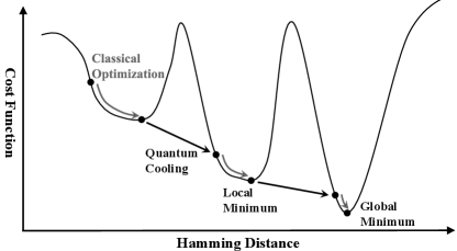
We proposed a hybrid quantum-classical algorithm to address this bottleneck. The entire algorithm functions as a heterogeneous cooling process to minimize the value of the cost function that encodes the given problem. The classical optimization is employed to find local minima, while the quantum cooling helps to escape the local minima by tunneling through energy barriers [1]. By alternating between classical optimization and quantum cooling, one can ultimately reach the global minimum. (See Fig.1 for a visualization of this process.)
In the classical part of the algorithm, well-established classical techniques, such as Monte Carlo or gradient descent, are used to identify a local minimum of the cost function with minor computational resources. In the quantum part of the algorithm, the quantum icebox algorithm (QIA) performs the quantum cooling, which has been shown to achieve quantum advantage in the unsorted search problem [2]. The framework of QIA is as follows. The cost function is encoded in a Hamiltonian system [3, 4], which is initialized in the state corresponding to the local minimum. A quantum bath has a trivial and easy-to-prepare ground states that is initialized within it. The system and the bath are coupled and maintain coherence, which facilitates coordinative quantum tunneling over high-energy barriers. The system will evolve to escape the local minimum and transition to a lower value. These two parts are complementary in order to prevent the algorithm from getting stuck.
Other hybrid quantum-classical algorithms [5, 6, 7, 8, 9, 10, 11, 12, 13, 14, 15] also combine classical and quantum methods as a compromise in the noisy intermediate-scale quantum (NISQ) era [16, 17], such as the variational quantum algorithm (VQA). In VQA, classical algorithms optimize the quantum gate parameters to reduce the number of quantum operations during the coherence time [18]. However, this approach faces challenges such as the barren plateau [9, 19] and the need to avoid local minima. In our scheme, the classical algorithm only needs to optimize the initial state and find local minima, which is less problematic. Furthermore, control channels are not required during QIA, which helps to minimize noise from external sources.
We specifically target a category of problems where the cost function involves Boolean variables [20, 21], such as the 3-SAT problem and independent sets [22, 23]. In physical terms, these cost functions represent Hamiltonians of (pseudo-)spins [24, 25]. The configuration space for these problems consists of binary strings of zeros and ones (or for spins), with each string representing a state . Local minima for this class of problems are defined as states where neighboring states within one Hamming distance have higher cost function values (or energies). The Hamming distance is calculated by counting the number of different bits between two binary strings [26]. To solve these problems, our hybrid quantum-classical algorithm operates as follows (see also Fig. 1) :
-
1.
Use arbitrary configuration as the initial condition to find out one of the local minima with classical algorithms.
-
2.
Prepare the quantum state in the computational basis, denoted as , and execute the QIA. Following quantum evolution, we obtain an entangled state . We then proceed to measure the problem system in the computational basis, resulting in the random selection of a configuration denoted as .
-
3.
Use the configuration as the initial condition to identify a different local minimum, represented as , using classical algorithms.
-
4.
If , then we update the initial configuration from to . In any case, we repeat the process starting from step 2.
-
5.
Stop the iteration if is sufficiently small and no further update to is available.
This hybrid quantum-classical algorithm is robust to noise and errors. The long Hamming distance tunneling is divided into several shorter Hamming distance tunnelings among local minima, making it suitable for qubits with limited coherence time. Furthermore, it can identify errors in step 4 and correct them through multiple rounds of optimization. These properties make it feasible to apply them practically and implement them experimentally.
With the assistance of classical algorithms, it can efficiently reduce local energy. This hybrid algorithm achieves quantum acceleration in step 2 by utilizing the quantum bath for efficient global cooling. We can also implement continuous quantum error correction [27, 28] or insert discrete quantum error correction [29, 30] in step 2 to suppress errors. We will demonstrate that using the quantum bath leads to higher cooling efficiency.
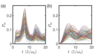
Since classical algorithms are well-established, let us now focus on the quantum component. We will compare the cooling efficiency of the quantum coherence bath with that of the classical bath to demonstrate the quantum advantage, particularly in the context of spin glasses. Spin glasses are typically challenging to cool down because they often have numerous local minima. Our numerical calculations demonstrate that the quantum coherence bath has a faster cooling speed and a higher success rate in comparison to the classical bath (see Fig. 2).
To achieve cooling, ancilla interacting qubits are commonly used as the quantum bath [2, 31, 32, 33]. However, this approach often requires at least twice the number of qubits [2, 31], and maintaining entanglement among a large number of qubits is difficult in the NISQ era [16, 17]. As an alternative, we use a coherent cavity as the quantum bath, which is more feasible than using hundreds of qubits. The cavity is typically used in experiments to propagate interactions [34, 35] or measure states [36], and can take the form of a laser cavity [37, 38], inductor-capacitor () oscillator [36], or nanomechanical resonator [39].
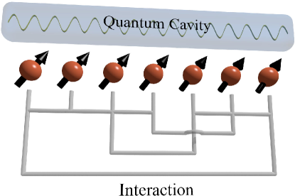
Our discussion will focus on the circuit quantum electrodynamics (cQED) systems [36], although our algorithm can also be applied to other systems. The basic setup is depicted in Fig. 3, where the cavity in the superconductor circuit can be modeled as an oscillator. The angular frequency of the oscillator is given by , where is the inductance and is the capacitance. The quantum cavity acts as the bath, and its Hamiltonian is
| (1) |
where is the creator of the harmonic mode of the bath.
The qubits in Josephson junctions store the problem data, and their interactions are established through circuit connections. The Hamiltonian encoding the problem of qubits is given by [40, 41, 42, 43, 44]
| (2) |
which describes a spin glass that is difficult to cool down. The on-site energy is denoted by , while represents the interaction between two qubits. This interaction can be spatially non-local, making the optimization problem more challenging. To facilitate quantum transitions, and are multiples of . The occurrence of integer multiple gaps is common when encoding discrete mathematical problems, including non-deterministic polynomial (NP) problems [3]. It also helps to suppress overflow errors caused by unencoded energy levels.
The interaction between the qubits and the cavity in the lumped-element circuit without spatial dependence is given by [45, 46, 36, 47, 48]
| (3) |
where is the interaction strength proportional to the capacitance. The interconnected capacitor introduces additional on-site capacitance, which can be absorbed in the parameters of and . Our scheme involves that is comparable to , resulting in acceleration and novel phenomena beyond perturbation approach, including rotating wave approximation (RWA) [49, 50, 51].
The cooling process is governed by the fixed total Hamiltonian with little additional control. The circuit diagram is available in Appendix A. The total parity conservation can slightly simplify the numerical simulation.
The initial state of the bath is its ground state [52, 53], and the initial state of the problem system is set to be one of the high energy local minima of in the -basis. Subsequently, the interaction is turned on, and the state evolves according to the Schrödinger equation. The energy of the system is absorbed by the bath through quantum tunneling, leading to the transfer of the system’s state to other local minima with lower energy.
For comparison, we treat the cavity as a classical system by defining the generalized momentum and the generalized position [36]. If the decoherence is strong, we can treat them as classical variables and [54, 55, 56, 57]. The Hamiltonians for the bath in Eq. (1) and the interaction in Eq. (3) can be rewritten, respectively, as
| (4) |
and
| (5) |
With the canonical equations and [58], we derive the total dynamical equations as
| (6) | |||||
| (7) | |||||
| (8) |
Notice that is the fixed point if all the qubits are aligned in the direction. The classical bath can be treated as a classical probability ensemble. For a fair comparison, the initial state of and is set to have the same probability distribution as the quantum ground state, which is with and [55, 56]. The expectation value is considered as the average of all the independent evolution paths, i.e., , where is the observable for one initial condition and is the expectation value.
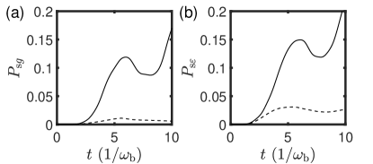
No entanglement exists between the classical bath and the system, and the initial state of the bath can be regarded as a mixed state. Throughout the evolution, the formation of entanglement is prohibited, and the total system remains in the product state . Moreover, some high energy paths of the classical bath are also not allowed, even though they could help the problem system surmount barriers. The numerical results depicted in Fig. 2 demonstrate that the classical bath performs worse than its quantum counterpart.
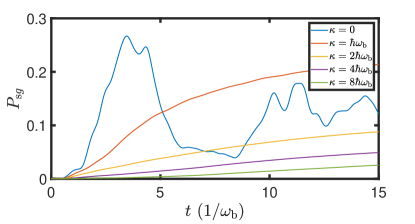
We simulate a problem system with two local minima using Eq. (2). The initial state of the problem system is at the higher local minimum, while the bath is in its ground state. The Hamming distance between the local minima is , which increases the problem complexity. Cooling with the quantum bath does not always outperform the classical bath, but quantum resonance can strongly accelerate cooling when is tuned suitably [59]. Fig. 2 shows the probability of the ground state changing over time. Cooling with the classical bath exhibits a modest increase over time, while the curve for the quantum bath shows a sharp increase due to quantum coherent enhancement. It indicates that QIA has an advantage in escaping local minima.
This quantum acceleration is related to the entanglement and correlation numerically calculated in Appendix B. In the continuous variable system, we also find a similar quantum acceleration (see Appendix C).
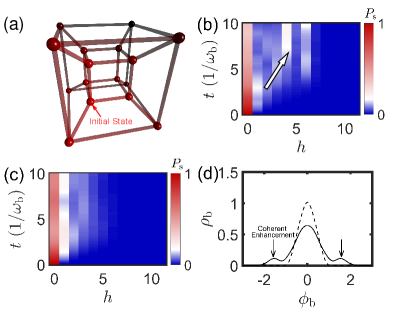
The eigenstates of the spin glass problem system are represented by a hypercube whose vertices correspond to the eigenstates in the basis as shown in Fig. 4(a). When the interaction is turned on, the wave function diffuses in the hypercube. As depicted in Fig. 4(b), the diffusion during quantum cooling is complex with peaks at the diffusion fronts, enabling faster reaching of the answers similar to diffusion in quantum walks (QWs) [59, 60, 61, 62]. On the other hand, the diffusion during classical cooling is weaker, and the probability distribution decreases monotonically with Hamming distance like the classical random walk (RW). These observations are depicted in Fig. 4(c).
Diffusion also occurs in the bath, leading to its state being driven away from its energy minimum. Better cooling performance is achieved when the bath is excited to higher energy states with greater probability and speed. Fig. 4(d) shows that the diffusion of the quantum bath is stronger with two peaks at the diffusion fronts, similar to the QW. On the other hand, the diffusion of the classical bath is weaker with monotonically decreasing fronts, as shown in Fig. 4(d). The classical bath diffuses very little without quantum coherence.
The diffusion in quantum cooling is similar to QW, as shown by the numerical results. To further illustrate this similarity, we consider a one qubit system with and . It is the Jaynes–Cummings model of non-rotating wave form [36]. There are analytical results in the regime that one of the parameters , or is much smaller than the others [63]. The non-perturbative resonant regime has rare analytical results. When the interaction is strong enough, an effective QW is observed in the dynamics. For a small time interval [64], its unitary evolution is (see Appendix D for derivation)
| (9) |
where the on-site energy is . For a typical Hadamard walk in a one-dimensional space with a coin qubit, its unitary operation of each iteration is , where is the Hadamard gate to the coin qubit and is the conditional walking operator controlled by the coin qubit. Therefore, in comparison, our system has an additional punishment term that may disturb the phase [59]. However, this punishment term disappears when the eigenstates of involved in the evolution are degenerate. This is exactly the case that we have studied where and are in resonance with matching energy gaps. It is well known that the average walking distance of RW is proportional to the square root of time while that of QW is proportional to the time [61, 65]. The constructive interference makes QW diffuse faster than RW. It is also known that the entanglement between the coin qubit and the walking space is strong.
For the QW with multiple coin qubits, the situation is more complex (see Appendix D). The analytical results always require non-local operation, such as the Grover’s coin [66, 67]. However, in our physical model, all the interactions are two-local. The numerical results in Fig. 4 suggests that QW still makes contribution in this complex case.
The quantum advancement of escaping local minima can be quantitatively approach. The numerical simulation of time complexity can be seen in Fig. 5, which the size of the Hilbert space is . The time required for QIA to transition between local minima is approximately when solving specific local interaction problems (further details in Appendix E). There are energy levels for the degenerate Hamiltonian which is proportional to the number of iterations and calls of the classical algorithm. So the total time complexity is about . Besides, there are connections to each qubit, so the total space complexity is .
The concept of using a cavity for cooling has similarities to the quantum-circuit refrigerator (QCR) [68, 69, 70], which utilizes an open cavity to cool a system. However, the QCR exhibits strong dissipation in the cavity, and some schemes utilize a dissipative qubit as the bath [71, 72]. Although an open bath can introduce steady energy loss, the lack of quantum coherence may hinder the cooling process. Recent research suggests that the non-Markovian baths could improve the performance of a quantum refrigerator [73, 74]. In Appendix F, we show that the dissipation in the quantum bath will slow down the cooling speed.
In conclusion, we proposed a hybrid quantum-classical algorithm of coherent cooling to address the issue of local minima. It encodes the cost function in a superconductor circuit cooled by a quantum cavity, which outperforms a classical cavity due to the coordinative tunneling effect. Our results suggest that the faster diffusion of QW over classical RW is the underlying physics of this quantum speed-up. While we have focused on discrete variable problems, our scheme can be extended to continuous variable problems. This hybrid algorithm is expected to streamline the control and reduce noise in quantum computing experiments.
Acknowledgements.
BW and JJF are supported by the National Key R&D Program of China (Grants No. 2017YFA0303302, No. 2018YFA0305602), National Natural Science Foundation of China (Grant No. 11921005), and Shanghai Municipal Science and Technology Major Project (Grant No.2019SHZDZX01).Appendix A Superconductor Circuit of Coherent Cooling
Superconductor circuits can be utilized to physically implement the quantum icebox algorithm, and we can use the simplest charge qubits of Josephson junction as an example as shown in Fig. 6. Other types of qubits require slight modifications. For phase qubits, an additional injected current is needed for each qubit. For flux qubits, the on-site capacitors are replaced by inductors, and the interconnected capacitors are replaced by mutual inductors [75, 42, 76]. The on-site energy can be tuned by the parallel capacitance of each qubit, while the interaction depends on the connectivity and coupling strength of the circuit matrix. The interaction is usually achieved by effective indirect interaction [77, 40, 42]. If the coherence of long-distance interaction is poor, indirect interaction can be used to improve it [78, 79, 34, 35, 80, 81, 82]. The crosstalk can be suppressed by a thick insulating layer made of high dielectric constant materials [80].
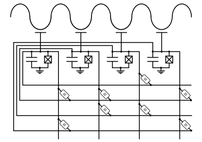
The design shown in Fig. 6 is inspired by the matrix circuit, a design commonly used in classical circuits for devices like screens, keyboards, and memories. The information is encoded in the intersections of the rows and columns, and only two circuit layers are needed. IBM have already realized the multi-layer chip of quantum computer, while there are tens of layers used in modern classical CPUs.
Appendix B The Influence of Strong Interaction
For quantum acceleration, strong interaction is required to overcome localization, which typically occurs in low-symmetry quantum systems and suppresses the propagation of wave functions [83, 84].
We begin by examining the eigenstates of the total Hamiltonian . In the absence of interaction (=0), the eigenstates are product states of the system and bath. The system is fully localized at the vertex of the hypercube in the basis, with no nearby probability distribution. If localization decreases, probability distribution appears nearby, and the peak of probability decreases as the probability is shared with other states. Thus, localization strength can be determined by of eigenstates with low energy, shown in Fig. 7(a). Weak interaction () results in highly localized eigenstates [84], as seen on the left side of Fig. 7(a), where the wave function is unable to reach the whole Hilbert space, preventing solution discovery. On the other hand, Strong interaction causes delocalization [59, 85, 86], as shown on the right side of Fig. 7(a), with sufficient probability distribution around the ground state.
Furthermore, the degree of localization can also impact the strength of revivals. Revivals typically occur in (pseudo-)integrable systems, where the state after evolution partially returns to its initial state. When the interaction is weak, only a few states are involved, resulting in strong revivals as illustrated by the dashed line in Fig. 7(b). On the other hand, when the interaction is comparable to the on-site energy, more states are involved, leading to a rich energy spectrum of the initial state, and weaker revivals as shown by the solid line in Fig. 7(b).
We use the entanglement entropy and correlation to further investigate the quantum coherence between the quantum bath and the problem system. The entanglement entropy is given by
| (10) |
where is the reduced density matrix of the problem system. The entanglement entropy is shown in Fig. 7(c). The correlation can be described by the joint probability defined as [87]
| (11) | |||||
Fig. 7(d) shows the correlation.
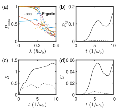
When the interaction between the problem system and the bath is weak (), the bath’s influence can be considered a perturbation. Thus, the composed system can be approximated as a product state of the problem system and the bath, and the rotating wave approximation (RWA) holds to a large extent. Both the entanglement entropy and correlation are small, as shown by the dashed lines in Figure 7. In this scenario, the localization is strong, but the cooling efficiency is low [84].
As the interaction strength becomes comparable with the on-site energy, , the composed system undergoes a phase transition [88] and the wave function becomes delocalized and ergodic [85, 86]. The product state approximation of the problem system and the bath is no longer valid. The entanglement and correlation between them increase significantly as depicted by the solid lines in Fig. 7, while the entanglement between the system and the classical bath is absent.
At the extremely strong coupling regime, the interaction dominates the dynamics. Despite the strong entanglement and correlation, the information from the system with is limited. Consequently, the cooling effect will vanish, leading to a low success rate.
Appendix C Cooling the Continuous System
For problems with continuous dynamical variables, they can also be encoded in Hamiltonians, for example, by mapping the variables to the generalized positions of Josephson junctions. The cost function for such a problem can be encoded in a Hamiltonian like this:
| (12) |
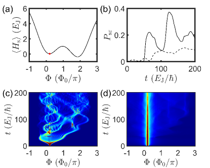
where is the external magnetic flux, is the quantum magnetic flux, is the inductance, and is the Josephson energy. These parameters can all be tuned [89]. The goal is to find the global minimum on , with the shape of the cost function shown in Fig. 8(a). The initial state is set at the higher local minimum.
The system-bath interaction can arise via the capacitor connection. This interaction can be described by the Hamiltonian
| (13) |
where is the effective capacitance of the connection. The influence of the on-site capacitance has already been included in parameters of and .
Cooling process with the quantum bath satisfies the Schrödinger equation. Cooling process using the classical bath satisfies the following equations
| (14) | |||||
| (15) | |||||
| (16) |
Comparing the time evolutions in Fig. 8(b), it is observed that the quantum bath yields better cooling efficiency than the classical bath in the continuous variable scenario. The quantum cooling displays characteristic quantum oscillations, while classical cooling is smoother. Fig. 8(c) illustrates the coherent diffusion of quantum cooling through coordinative tunneling in the position space, displaying strong coherent enhancement at the wave function’s fronts. Fig. 8(d) shows the smoother incoherent diffusion of classical cooling, with the strongest component trapped in the higher local minimum.
Appendix D Quantum Walk Effect in the Coherent Cooling
Governed by the Schrödinger equation, the time evolution of the composed Hamiltonian can be divided into small steps
| (17) |
The unitary operator for each step, for the Hamiltonian in Eq. (9) in the main text, can be approximated as [64]
where we have omitted all the terms. The dimensionless operator is . Notice that the angle of rotation axis between and of the coin qubit is in the Hadamard walk. In the time interval , this condition will be satisfied with
| (19) |
Then the rotation axis between the last two terms is also . To simplify the comparison with the Hadamard walk, we do the transformation that
| (20) |
Then the operation becomes
| (21) |
When , namely, , the last term is the Hadamard gate. Moreover, the displacement of conditional translation is , so the self-consistent requires . In summary, the unitary operation is
| (22) |
Except the term , it is just the standard Hadamard walk.
In the case of spin glass with multi-qubits, the operation is
| (23) |
where the Hadamard gates require . The conditional walker is more complex that
Appendix E Time Complexity
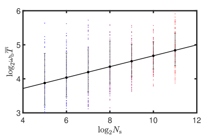
In this section, we will attempt to evaluate the time complexity of our algorithm. Our algorithm is general and applicable to many optimization problems. However, in order to gain informative results with limited computational resources, we need to narrow our focus to a specific set of problems. These optimization problems are constructed in the following manner. All qubits are first connected in a one-dimensional chain to make them inseparable. We then connect each qubit to another randomly selected qubit. The number of links for each qubit ranges from 2 to , with an average of links per qubit. Ferromagnetic interaction exists only between two connected qubits with equal strength. As a result, there are two global minima and . Finally, we add on-site energy to certain qubits. The two ground states will split: one becomes a local minimum with high-energy and the other remains a global minimum.
For a system with qubits, it can correspond to a graph. As there are different graphs, and the configuration space is extremely large. It is difficult to traverse all of the graphs. As a compromise, we sample one hundred graphs following the mentioned rule for each value of and consider them as typical.
If the problem system reaches the global minimum, we consider the cooling process successful, which can be described by the characteristic time and the success rate . The characteristic time refers to the speed at which the dynamics reach equilibrium. The success rate is the total probability at the global minimum when the dynamics reach equilibrium. To extract the characteristic time and success rate, we fit the numerical results with the following function
| (25) |
where the function has the properties that and . Using the fitting function can suppress the poisoning of the results caused by accidental narrow peaks and outliers. Here, we have chosen the fitting function to be , where is the zero-order Bessel function of the first kind. The fitting performance is shown in Fig. 9. Since there are only two free parameters, the fitting may not be perfect. Other fitting functions are tried, yielding parameters of similar magnitude.
Now, we will begin analyzing the time complexity. The average running time can be defined as
| (26) |
where is the characteristic time of the dynamics and is the success rate. is approximately proportional to the runtime required to achieve a given success rate. If is smaller, more attempts and measurements will be required. If the interaction is exceedingly strong, the system will rapidly become ergodic. However, there is no calculation associated with this type of probability increment. So, we subtract the background probability of such a wild guess, which is . The average running time against the system’s size is shown in Fig. 5. The best and worst cases are not shown because they are difficult to sample with a large value of . For the average case in samples, the regression yields a gradient of approximately 0.16. The time complexity for each successful cooling is .
The encoding Hamiltonian is highly degenerate with energy levels. The maximum number of iterations required to reach the lowest energy levels is also bounded by . Specifically, it is for solving the maximal independent set problem with the two-local Hamiltonian.
In summary, the total average time complexity is approximately . The time complexity of the classical algorithm is approximately [90].
Appendix F Decoherence with Markov Master Equation
In the main text, we have discussed cooling with a coherent quantum bath using the Schrödinger equation. However, the experiment always faces decoherence, such as the thermal bath, which has been shown to easily reach local minima [91]. Now we investigate the ability to reach the global minimum and treat the cooling with the Markov master equation [92, 93]
| (27) |
where represents the decoherence strength of the bath. In Fig. 10, we compare the cooling processes with different values of . The case with corresponds to the case discussed in the main text.
The numerical results indicate that the cooling process without decoherence is faster in the early stage. Although decoherence can extract energy from the bath irreversibly, it can disrupt the quantum acceleration by suppressing the off-diagonal terms of the density matrix . This transition between quantum states requires these off-diagonal terms, and the present of decoherence can hinder quantum tunneling.
At the late cooling stage, the cooling process reaches saturation. Even a small amount of decoherence can decrease the revival from quantum oscillation [94, 83]. Strong decoherence, on the other hand, can entirely suppress the quantum transition.
We consider a simple case to demonstrate the effect of decoherence on quantum acceleration, where both the problem system and the bath are two-level systems [73, 74]. The states are re-defined as , , and . Eq. (27) in RWA can then be written as
| (28) | |||||
| (29) | |||||
| (30) | |||||
| (31) |
where . The initial condition is and other elements of the density matrix are zero. The solution is
| (32) | |||||
where and . It is a damped oscillator with the decoherence slowing down the oscillation angular frequency from to . As a result, the quantum transition between and is also slowed down.
When the decoherence is small , the system is in the underdamped regime with oscillations. The probability of being in the ground state is approximately given by
| (33) |
In the early stage , Eq. (33) can be simplified to
| (34) |
The last term is due to decoherence, and its negativity implies that it leads to deceleration.
When , the system is in the overdamped regime without oscillations, and the ground state probability is given by
| (35) |
which indicates that stronger decoherence leads to slower cooling. In this regime, the bath is almost frozen in its ground state, and the dynamics are essentially static.
References
- Espinosa [2019] J. R. Espinosa, Tunneling without bounce, Phys. Rev. D 100, 105002 (2019).
- Feng et al. [2022] J.-J. Feng, B. Wu, and F. Wilczek, Quantum computing by coherent cooling, Phys. Rev. A 105, 052601 (2022).
- Farhi et al. [2001] E. Farhi, J. Goldstone, S. Gutmann, J. Lapan, A. Lundgren, and D. Preda, A quantum adiabatic evolution algorithm applied to random instances of an np-complete problem, Science 292, 472 (2001).
- Ebadi et al. [2022] S. Ebadi, A. Keesling, M. Cain, T. T. Wang, H. Levine, D. Bluvstein, G. Semeghini, A. Omran, J.-G. Liu, R. Samajdar, X.-Z. Luo, B. Nash, X. Gao, B. Barak, E. Farhi, S. Sachdev, N. Gemelke, L. Zhou, S. Choi, H. Pichler, S.-T. Wang, M. Greiner, V. Vuletić, and M. D. Lukin, Quantum optimization of maximum independent set using rydberg atom arrays, Science 376, 1209 (2022).
- Farhi et al. [2014] E. Farhi, J. Goldstone, and S. Gutmann, A quantum approximate optimization algorithm (2014), arXiv:1411.4028 [quant-ph] .
- Peruzzo et al. [2014] A. Peruzzo, J. McClean, P. Shadbolt, M.-H. Yung, X.-Q. Zhou, P. J. Love, A. Aspuru-Guzik, and J. L. O’Brien, A variational eigenvalue solver on a photonic quantum processor, Nature Communications 5, 4213 (2014).
- McClean et al. [2016] J. R. McClean, J. Romero, R. Babbush, and A. Aspuru-Guzik, The theory of variational hybrid quantum-classical algorithms, New Journal of Physics 18, 023023 (2016).
- Colless et al. [2018] J. I. Colless, V. V. Ramasesh, D. Dahlen, M. S. Blok, M. E. Kimchi-Schwartz, J. R. McClean, J. Carter, W. A. de Jong, and I. Siddiqi, Computation of molecular spectra on a quantum processor with an error-resilient algorithm, Phys. Rev. X 8, 011021 (2018).
- McClean et al. [2018] J. R. McClean, S. Boixo, V. N. Smelyanskiy, R. Babbush, and H. Neven, Barren plateaus in quantum neural network training landscapes, Nature Communications 9, 4812 (2018).
- McArdle et al. [2019] S. McArdle, T. Jones, S. Endo, Y. Li, S. C. Benjamin, and X. Yuan, Variational ansatz-based quantum simulation of imaginary time evolution, npj Quantum Information 5, 75 (2019).
- Zhou et al. [2020] L. Zhou, S.-T. Wang, S. Choi, H. Pichler, and M. D. Lukin, Quantum approximate optimization algorithm: Performance, mechanism, and implementation on near-term devices, Phys. Rev. X 10, 021067 (2020).
- Cerezo et al. [2021] M. Cerezo, A. Sone, T. Volkoff, L. Cincio, and P. J. Coles, Cost function dependent barren plateaus in shallow parametrized quantum circuits, Nature Communications 12, 1791 (2021).
- Endo et al. [2021] S. Endo, Z. Cai, S. C. Benjamin, and X. Yuan, Hybrid quantum-classical algorithms and quantum error mitigation, Journal of the Physical Society of Japan 90, 032001 (2021).
- Xin et al. [2021] T. Xin, L. Che, C. Xi, A. Singh, X. Nie, J. Li, Y. Dong, and D. Lu, Experimental quantum principal component analysis via parametrized quantum circuits, Phys. Rev. Lett. 126, 110502 (2021).
- Wang et al. [2023] Z. Wang, P.-L. Zheng, B. Wu, and Y. Zhang, Quantum dropout: On and over the hardness of quantum approximate optimization algorithm, Phys. Rev. Res. 5, 023171 (2023).
- Preskill [2018] J. Preskill, Quantum Computing in the NISQ era and beyond, Quantum 2, 79 (2018).
- Bharti et al. [2022] K. Bharti, A. Cervera-Lierta, T. H. Kyaw, T. Haug, S. Alperin-Lea, A. Anand, M. Degroote, H. Heimonen, J. S. Kottmann, T. Menke, W.-K. Mok, S. Sim, L.-C. Kwek, and A. Aspuru-Guzik, Noisy intermediate-scale quantum algorithms, Rev. Mod. Phys. 94, 015004 (2022).
- Cao et al. [2019] Y. Cao, J. Romero, J. P. Olson, M. Degroote, P. D. Johnson, M. Kieferová, I. D. Kivlichan, T. Menke, B. Peropadre, N. P. D. Sawaya, S. Sim, L. Veis, and A. Aspuru-Guzik, Quantum chemistry in the age of quantum computing, Chemical Reviews 119, 10856 (2019).
- Gil-Fuster et al. [2023] E. Gil-Fuster, J. Eisert, and C. Bravo-Prieto, Understanding quantum machine learning also requires rethinking generalization (2023), arXiv:2306.13461 [quant-ph] .
- Bollig and Wegener [1996] B. Bollig and I. Wegener, Improving the variable ordering of obdds is np-complete, IEEE Transactions on Computers 45, 993 (1996).
- Kolmogorov and Zabin [2004] V. Kolmogorov and R. Zabin, What energy functions can be minimized via graph cuts?, IEEE Transactions on Pattern Analysis and Machine Intelligence 26, 147 (2004).
- Tovey [1984] C. A. Tovey, A simplified np-complete satisfiability problem, Discrete Applied Mathematics 8, 85 (1984).
- Sakai et al. [2003] S. Sakai, M. Togasaki, and K. Yamazaki, A note on greedy algorithms for the maximum weighted independent set problem, Discrete Applied Mathematics 126, 313 (2003).
- Hu et al. [2021] Y. Hu, Z. Zhang, and B. Wu, Quantum algorithm for a set of quantum 2sat problems, Chinese Physics B 30, 020308 (2021).
- Yu et al. [2021] H. Yu, F. Wilczek, and B. Wu, Quantum algorithm for approximating maximum independent sets, Chinese Physics Letters 38, 030304 (2021).
- Trugenberger [2001] C. A. Trugenberger, Probabilistic quantum memories, Phys. Rev. Lett. 87, 067901 (2001).
- Ahn et al. [2003] C. Ahn, H. M. Wiseman, and G. J. Milburn, Quantum error correction for continuously detected errors, Phys. Rev. A 67, 052310 (2003).
- Livingston et al. [2022] W. P. Livingston, M. S. Blok, E. Flurin, J. Dressel, A. N. Jordan, and I. Siddiqi, Experimental demonstration of continuous quantum error correction, Nature Communications 13, 2307 (2022).
- Fowler et al. [2012] A. G. Fowler, M. Mariantoni, J. M. Martinis, and A. N. Cleland, Surface codes: Towards practical large-scale quantum computation, Phys. Rev. A 86, 032324 (2012).
- Bluvstein et al. [2023] D. Bluvstein, S. J. Evered, A. A. Geim, S. H. Li, H. Zhou, T. Manovitz, S. Ebadi, M. Cain, M. Kalinowski, D. Hangleiter, J. P. B. Ataides, N. Maskara, I. Cong, X. Gao, P. S. Rodriguez, T. Karolyshyn, G. Semeghini, M. J. Gullans, M. Greiner, V. Vuletić, and M. D. Lukin, Logical quantum processor based on reconfigurable atom arrays, Nature 10.1038/s41586-023-06927-3 (2023).
- Matthies et al. [2022] A. Matthies, M. Rudner, A. Rosch, and E. Berg, Programmable adiabatic demagnetization for systems with trivial and topological excitations (2022), arXiv:2210.17256 [quant-ph] .
- Rodríguez-Briones and Laflamme [2016] N. A. Rodríguez-Briones and R. Laflamme, Achievable polarization for heat-bath algorithmic cooling, Phys. Rev. Lett. 116, 170501 (2016).
- Zaiser et al. [2021] S. Zaiser, C. T. Cheung, S. Yang, D. B. R. Dasari, S. Raeisi, and J. Wrachtrup, Cyclic cooling of quantum systems at the saturation limit, npj Quantum Information 7, 92 (2021).
- Majer et al. [2007] J. Majer, J. M. Chow, J. M. Gambetta, J. Koch, B. R. Johnson, J. A. Schreier, L. Frunzio, D. I. Schuster, A. A. Houck, A. Wallraff, A. Blais, M. H. Devoret, S. M. Girvin, and R. J. Schoelkopf, Coupling superconducting qubits via a cavity bus, Nature 449, 443 (2007).
- Blais et al. [2007] A. Blais, J. Gambetta, A. Wallraff, D. I. Schuster, S. M. Girvin, M. H. Devoret, and R. J. Schoelkopf, Quantum-information processing with circuit quantum electrodynamics, Phys. Rev. A 75, 032329 (2007).
- Blais et al. [2021] A. Blais, A. L. Grimsmo, S. M. Girvin, and A. Wallraff, Circuit quantum electrodynamics, Rev. Mod. Phys. 93, 025005 (2021).
- Kurizki et al. [2015] G. Kurizki, P. Bertet, Y. Kubo, K. Mølmer, D. Petrosyan, P. Rabl, and J. Schmiedmayer, Quantum technologies with hybrid systems, Proceedings of the National Academy of Sciences 112, 3866 (2015).
- Aspelmeyer et al. [2014] M. Aspelmeyer, T. J. Kippenberg, and F. Marquardt, Cavity optomechanics, Rev. Mod. Phys. 86, 1391 (2014).
- Cleland and Geller [2004] A. N. Cleland and M. R. Geller, Superconducting qubit storage and entanglement with nanomechanical resonators, Phys. Rev. Lett. 93, 070501 (2004).
- Collodo et al. [2020] M. C. Collodo, J. Herrmann, N. Lacroix, C. K. Andersen, A. Remm, S. Lazar, J.-C. Besse, T. Walter, A. Wallraff, and C. Eichler, Implementation of conditional phase gates based on tunable interactions, Phys. Rev. Lett. 125, 240502 (2020).
- Lucas [2014] A. Lucas, Ising formulations of many np problems, Frontiers in Physics 2, 10.3389/fphy.2014.00005 (2014).
- Zhao et al. [2020] P. Zhao, P. Xu, D. Lan, J. Chu, X. Tan, H. Yu, and Y. Yu, High-contrast interaction using superconducting qubits with opposite-sign anharmonicity, Phys. Rev. Lett. 125, 200503 (2020).
- Gong et al. [2021] M. Gong, S. Wang, C. Zha, M.-C. Chen, H.-L. Huang, Y. Wu, Q. Zhu, Y. Zhao, S. Li, S. Guo, H. Qian, Y. Ye, F. Chen, C. Ying, J. Yu, D. Fan, D. Wu, H. Su, H. Deng, H. Rong, K. Zhang, S. Cao, J. Lin, Y. Xu, L. Sun, C. Guo, N. Li, F. Liang, V. M. Bastidas, K. Nemoto, W. J. Munro, Y.-H. Huo, C.-Y. Lu, C.-Z. Peng, X. Zhu, and J.-W. Pan, Quantum walks on a programmable two-dimensional 62-qubit superconducting processor, Science 372, 948 (2021).
- King et al. [2022] A. D. King, S. Suzuki, J. Raymond, A. Zucca, T. Lanting, F. Altomare, A. J. Berkley, S. Ejtemaee, E. Hoskinson, S. Huang, E. Ladizinsky, A. J. R. MacDonald, G. Marsden, T. Oh, G. Poulin-Lamarre, M. Reis, C. Rich, Y. Sato, J. D. Whittaker, J. Yao, R. Harris, D. A. Lidar, H. Nishimori, and M. H. Amin, Coherent quantum annealing in a programmable 2000 qubit ising chain, Nature Physics 18 (2022).
- Gely et al. [2017] M. F. Gely, A. Parra-Rodriguez, D. Bothner, Y. M. Blanter, S. J. Bosman, E. Solano, and G. A. Steele, Convergence of the multimode quantum rabi model of circuit quantum electrodynamics, Phys. Rev. B 95, 245115 (2017).
- Malekakhlagh et al. [2017] M. Malekakhlagh, A. Petrescu, and H. E. Türeci, Cutoff-free circuit quantum electrodynamics, Phys. Rev. Lett. 119, 073601 (2017).
- Miyanaga et al. [2021] T. Miyanaga, A. Tomonaga, H. Ito, H. Mukai, and J. Tsai, Ultrastrong tunable coupler between superconducting resonators, Phys. Rev. Applied 16, 064041 (2021).
- Altoé et al. [2022] M. V. P. Altoé, A. Banerjee, C. Berk, A. Hajr, A. Schwartzberg, C. Song, M. Alghadeer, S. Aloni, M. J. Elowson, J. M. Kreikebaum, E. K. Wong, S. M. Griffin, S. Rao, A. Weber-Bargioni, A. M. Minor, D. I. Santiago, S. Cabrini, I. Siddiqi, and D. F. Ogletree, Localization and mitigation of loss in niobium superconducting circuits, PRX Quantum 3, 020312 (2022).
- Kuzmin et al. [2019] R. Kuzmin, N. Mehta, N. Grabon, R. Mencia, and V. E. Manucharyan, Superstrong coupling in circuit quantum electrodynamics, npj Quantum Information 5, 20 (2019).
- Talkner and Hänggi [2020] P. Talkner and P. Hänggi, Colloquium: Statistical mechanics and thermodynamics at strong coupling: Quantum and classical, Rev. Mod. Phys. 92, 041002 (2020).
- Liu et al. [2021] J. Liu, K. A. Jung, and D. Segal, Periodically driven quantum thermal machines from warming up to limit cycle, Phys. Rev. Lett. 127, 200602 (2021).
- Um et al. [2016] M. Um, J. Zhang, D. Lv, Y. Lu, S. An, J.-N. Zhang, H. Nha, M. S. Kim, and K. Kim, Phonon arithmetic in a trapped ion system, Nature Communications 7, 11410 (2016).
- Schuster et al. [2007] D. I. Schuster, A. A. Houck, J. A. Schreier, A. Wallraff, J. M. Gambetta, A. Blais, L. Frunzio, J. Majer, B. Johnson, M. H. Devoret, S. M. Girvin, and R. J. Schoelkopf, Resolving photon number states in a superconducting circuit, Nature 445, 515 (2007).
- Caldeira and Leggett [1983] A. Caldeira and A. Leggett, Path integral approach to quantum brownian motion, Physica A: Statistical Mechanics and its Applications 121, 587 (1983).
- Polkovnikov [2010] A. Polkovnikov, Phase space representation of quantum dynamics, Annals of Physics 325, 1790 (2010).
- Curtright and Zachos [2012] T. L. Curtright and C. K. Zachos, Quantum mechanics in phase space, Asia Pacific Physics Newsletter 01, 37 (2012).
- Wang et al. [2021] Z. Wang, J. Feng, and B. Wu, Microscope for quantum dynamics with planck cell resolution, Phys. Rev. Research 3, 033239 (2021).
- Zhang and Wu [2006] Q. Zhang and B. Wu, General approach to quantum-classical hybrid systems and geometric forces, Phys. Rev. Lett. 97, 190401 (2006).
- Childs and Goldstone [2004] A. M. Childs and J. Goldstone, Spatial search by quantum walk, Phys. Rev. A 70, 022314 (2004).
- Childs [2009] A. M. Childs, Universal computation by quantum walk, Phys. Rev. Lett. 102, 180501 (2009).
- Venegas-Andraca [2012] S. E. Venegas-Andraca, Quantum walks: a comprehensive review, Quantum Information Processing 11, 1015 (2012).
- Liu et al. [2023] Y. Liu, W. J. Su, and T. Li, On Quantum Speedups for Nonconvex Optimization via Quantum Tunneling Walks, Quantum 7, 1030 (2023).
- Casanova et al. [2010] J. Casanova, G. Romero, I. Lizuain, J. J. García-Ripoll, and E. Solano, Deep strong coupling regime of the jaynes-cummings model, Phys. Rev. Lett. 105, 263603 (2010).
- Casas et al. [2012] F. Casas, A. Murua, and M. Nadinic, Efficient computation of the zassenhaus formula, Computer Physics Communications 183, 2386 (2012).
- Kempe [2003] J. Kempe, Quantum random walks: An introductory overview, Contemporary Physics 44, 307 (2003).
- Carneiro et al. [2005] I. Carneiro, M. Loo, X. Xu, M. Girerd, V. Kendon, and P. L. Knight, Entanglement in coined quantum walks on regular graphs, New Journal of Physics 7, 156 (2005).
- Shenvi et al. [2003] N. Shenvi, J. Kempe, and K. BirgittaWhaley, Quantum random-walk search algorithm, Phys. Rev. A 67, 052307 (2003).
- Tan et al. [2017] K. Y. Tan, M. Partanen, R. E. Lake, J. Govenius, S. Masuda, and M. Möttönen, Quantum-circuit refrigerator, Nat. Commun. 8, 15189 (2017).
- Silveri et al. [2017] M. Silveri, H. Grabert, S. Masuda, K. Y. Tan, and M. Möttönen, Theory of quantum-circuit refrigeration by photon-assisted electron tunneling, Phys. Rev. B 96, 094524 (2017).
- Hsu et al. [2020] H. Hsu, M. Silveri, A. Gunyhó, J. Goetz, G. Catelani, and M. Möttönen, Tunable refrigerator for nonlinear quantum electric circuits, Phys. Rev. B 101, 235422 (2020).
- Raghunandan et al. [2020] M. Raghunandan, F. Wolf, C. Ospelkaus, P. O. Schmidt, and H. Weimer, Initialization of quantum simulators by sympathetic cooling, Science Advances 6, eaaw9268 (2020).
- Polla et al. [2021] S. Polla, Y. Herasymenko, and T. E. O’Brien, Quantum digital cooling, Phys. Rev. A 104, 012414 (2021).
- Camati et al. [2020] P. A. Camati, J. F. G. Santos, and R. M. Serra, Employing non-markovian effects to improve the performance of a quantum otto refrigerator, Phys. Rev. A 102, 012217 (2020).
- Zhang et al. [2021] Q. Zhang, Z.-X. Man, and Y.-J. Xia, Non-markovianity and the landauer principle in composite thermal environments, Phys. Rev. A 103, 032201 (2021).
- Harris et al. [2009] R. Harris, T. Lanting, A. J. Berkley, J. Johansson, M. W. Johnson, P. Bunyk, E. Ladizinsky, N. Ladizinsky, T. Oh, and S. Han, Compound josephson-junction coupler for flux qubits with minimal crosstalk, Phys. Rev. B 80, 052506 (2009).
- Dai et al. [2021] X. Dai, D. Tennant, R. Trappen, A. Martinez, D. Melanson, M. Yurtalan, Y. Tang, S. Novikov, J. Grover, S. Disseler, J. Basham, R. Das, D. Kim, A. Melville, B. Niedzielski, S. Weber, J. Yoder, D. Lidar, and A. Lupascu, Calibration of flux crosstalk in large-scale flux-tunable superconducting quantum circuits, PRX Quantum 2, 040313 (2021).
- van den Brink et al. [2005] A. M. van den Brink, A. J. Berkley, and M. Yalowsky, Mediated tunable coupling of flux qubits, New Journal of Physics 7, 230 (2005).
- Qiu et al. [2020] X. Qiu, P. Zoller, and X. Li, Programmable quantum annealing architectures with ising quantum wires, PRX Quantum 1, 020311 (2020).
- Zhong et al. [2019] Y. P. Zhong, H. S. Chang, K. J. Satzinger, M. H. Chou, A. Bienfait, C. R. Conner, E. Dumur, J. Grebel, G. A. Peairs, R. G. Povey, D. I. Schuster, and A. N. Cleland, Violating bell’s inequality with remotely connected superconducting qubits, Nature Physics 15, 741 (2019).
- Zhao et al. [2022] P. Zhao, K. Linghu, Z. Li, P. Xu, R. Wang, G. Xue, Y. Jin, and H. Yu, Quantum crosstalk analysis for simultaneous gate operations on superconducting qubits, PRX Quantum 3, 020301 (2022).
- Kannan et al. [2020] B. Kannan, M. J. Ruckriegel, D. L. Campbell, A. Frisk Kockum, J. Braumüller, D. K. Kim, M. Kjaergaard, P. Krantz, A. Melville, B. M. Niedzielski, A. Vepsäläinen, R. Winik, J. L. Yoder, F. Nori, T. P. Orlando, S. Gustavsson, and W. D. Oliver, Waveguide quantum electrodynamics with superconducting artificial giant atoms, Nature 583, 775 (2020).
- Zhong et al. [2021] Y. Zhong, H.-S. Chang, A. Bienfait, E. Dumur, M.-H. Chou, C. R. Conner, J. Grebel, R. G. Povey, H. Yan, D. I. Schuster, and A. N. Cleland, Deterministic multi-qubit entanglement in a quantum network, Nature 590, 571 (2021).
- Schreiber et al. [2011] A. Schreiber, K. N. Cassemiro, V. Potoček, A. Gábris, I. Jex, and C. Silberhorn, Decoherence and disorder in quantum walks: From ballistic spread to localization, Phys. Rev. Lett. 106, 180403 (2011).
- Abanin et al. [2019] D. A. Abanin, E. Altman, I. Bloch, and M. Serbyn, Colloquium: Many-body localization, thermalization, and entanglement, Rev. Mod. Phys. 91, 021001 (2019).
- Potter et al. [2015] A. C. Potter, R. Vasseur, and S. A. Parameswaran, Universal properties of many-body delocalization transitions, Phys. Rev. X 5, 031033 (2015).
- Serbyn et al. [2015] M. Serbyn, Z. Papić, and D. A. Abanin, Criterion for many-body localization-delocalization phase transition, Phys. Rev. X 5, 041047 (2015).
- Zeng et al. [2019] B. Zeng, X. Chen, D.-L. Zhou, and X.-G. Wen, Quantum Information Meets Quantum Matter (Springer, New York, 2019).
- Luitz et al. [2015] D. J. Luitz, N. Laflorencie, and F. Alet, Many-body localization edge in the random-field heisenberg chain, Phys. Rev. B 91, 081103 (2015).
- Harris et al. [2010] R. Harris, J. Johansson, A. J. Berkley, M. W. Johnson, T. Lanting, S. Han, P. Bunyk, E. Ladizinsky, T. Oh, I. Perminov, E. Tolkacheva, S. Uchaikin, E. M. Chapple, C. Enderud, C. Rich, M. Thom, J. Wang, B. Wilson, and G. Rose, Experimental demonstration of a robust and scalable flux qubit, Phys. Rev. B 81, 134510 (2010).
- Xiao and Nagamochi [2017] M. Xiao and H. Nagamochi, Exact algorithms for maximum independent set, Information and Computation 255, 126 (2017).
- Chen et al. [2023] C.-F. Chen, H.-Y. Huang, J. Preskill, and L. Zhou, Local minima in quantum systems (2023), arXiv:2309.16596 [quant-ph] .
- Orszag and Retamal [2001] M. Orszag and J. Retamal, Modern Challenges in Quantum Optics (Springer, 2001).
- Li et al. [2023] X. Li, Y. Zhou, and H. Zhang, Manipulating atom-cavity interactions with configurable atomic chains (2023), arXiv:2308.07908 [quant-ph] .
- Kendon and Tregenna [2003] V. Kendon and B. Tregenna, Decoherence can be useful in quantum walks, Phys. Rev. A 67, 042315 (2003).