Error Floor of Spinal Codes under ML Decoding

Aimin Li , Graduate Student Member, IEEE, Shaohua Wu , Member, IEEE,
Xiaomeng Chen , Graduate Student Member, IEEE, and Sumei Sun , Fellow, IEEE This work has been supported in part by the National Key Research and Development Program of China under Grant no. 2020YFB1806403, and in part by the Guangdong Basic and Applied Basic Research Foundation under Grant no. 2022B1515120002, and in part by the Major Key Project of PCL under Grant no. PCL2024A01, and in part by the Shenzhen Science and Technology Program under Grant no. ZDSYS20210623091808025. (Corresponding author: Shaohua Wu.) A. Li and X. Chen are with the Department of Electronic Engineering, Harbin Institute of Technology (Shenzhen), Shenzhen, China 518055. E-mail: [email protected]; [email protected]. S. Wu is with the Department of Electronic Engineering, Harbin Institute of Technology (Shenzhen), Shenzhen, China 518055, and also with the Peng Cheng Laboratory, 518055, China. E-mail: [email protected]. S. Sun is with the Institute for Infocomm Research, Agency for Science, Technology and Research (A*STAR), Singapore 138632. Email: [email protected].

Abstract

Spinal codes is a new family of capacity-achieving rateless codes that has been shown to achieve better rate performance compared to Raptor codes, Strider codes, and rateless Low-Density Parity-Check (LDPC) codes. This correspondence addresses the performance limitations of Spinal codes in the finite block length regime, uncovering an error floor phenomenon at high Signal-to-Noise Ratios (SNRs). We develop an analytical expression to approximate the error floor and devise SNR thresholds at which the error floor initiates. Numerical results across Additive White Gaussian Noise (AWGN), rayleigh, and nakagami-m fading channels verify the accuracy of our analysis. The analysis and numerical results also show that transmitting more passes of symbols can lower the error floor but does not affect the SNR threshold, providing insights on the performance target, the working SNR region, and the code design.

Index Terms:

Rateless Codes, Spinal Codes, Error Floor, AWGN channel, Fading Channel.

I Introduction

Spinal codes, first introduced in 2011 [1], is the first rateless codes that has been theoretically proven to achieve the Shannon capacity over the Binary Symmetric Channel (BSC) and the AWGN channels [2]. Experimentally, Spinal codes has been shown to achieve higher rate compared to Raptor codes [3], Strider codes [4], and rateless Low-Density Parity-Check (LDPC) codes [5] across a wide range of channel conditions and message sizes [6].

Attributing to Spinal codes’ rateless, capacity-achieving nature, and superior rate performance under short message lengths, Spinal codes has received extensive attention in the coding theory community. Key areas of investigation include the design of coding structures [7, 8, 9, 10], development of high-efficiency decoding mechanisms [11, 12, 13, 14], applications in quantum information processing [15], optimizations of punctured codes [16, 17, 18], and Polar-Spinal concatenation improved codes [19, 20, 21, 22]. These studies offer deeper insights into Spinal codes. The excellent rate performance for short message length and the channel-adaptive rateless nature also make Spinal codes well-suited for deployment in 6G non-terrestrial networks (NTN) [23], which are expected to support a wide range of vehicle-to-vehicle (V2V) applications such as UAV networks [24, 25], deep space explorations [26], Low Earth Orbit (LEO) satellite communications [27], and satellite laser communications [28].

The theoretical performance analysis of Spinal codes, however, is still in an early stage (See Table I for an overview). In [2], the asymptotic performance of Spinal codes was investigated, proving that that Spinal codes is capacity-achieving. In [7] and [29], under the Finite Block-Length (FBL) regime, Yang, et.al derived the bounds on the Block Error Rate (BLER) of Spinal codes over the Binary Erasure Channel (BEC) and the AWGN channel, respectively. In [30], the upper bound on the BLER of Spinal codes over the AWGN channel was further tightened. In [10], the upper bound of Spinal codes over the rayleigh fading channel without Channel State Information (CSI) was derived. Then, in [31], tight upper bounds over rayleigh, rician, and nakagami-m fading channels under perfect CSI were explicitly derived. [32] further extends the result in [31] by deriving a unified FBL BLER upper bound for general channels, achieving consistent tightness across a wide range of channel conditions.

TABLE I: A Summary of Theoretical Analysis of Spinal Codes

Contribution	References
Asymptotic Analysis	[2]
FBL BLER Bound over AWGN	[7, 30]
FBL BLER Bound over BEC	[29]
FBL BLER Bound over Fading Channels	[18, 10, 31]
Error Floor Analysis	This work

While existing analyses have achieved precise approximations of Spinal codes’ performance, the error floor phenomenon—where increasing SNR does not yield further improvements in error probability—has not been rigorously studied. Such a phenomenon has been documented in many other typical channel codes like Polar codes [33, 34, 35] and LDPC codes [36, 37, 38, 39], with several efforts aimed at lowering the error floor [35, 37, 39].

Motivated by this gap, this correspondence reveals that Spinal codes suffers from an error floor. We present an explicit expression for the error floor and analyze the SNR thresholds that trigger the error floors across AWGN, nakagami-m fading channels, and rayleigh fading channels. The analysis and numerical results indicate that transmitting additional passes of symbols can reduce the error floor but cannot change the SNR threshold, which offers insights on the SNR working region, the performance target, and the design of codes.

II Preliminaries of Spinal Codes

II-A Encoding of Spinal Codes

The encoding process of Spinal codes is shown in Fig. 1:

1) Segmentation: Divide an $n$ -bit message $\mathbf{M}$ into $k$ -bit segments $\mathbf{m}_{i}\in\left\{0,1\right\}^{k}$ , where $i\in\{1,2,\cdots,n/k\}$ .

2) Sequentially Hashing: The hash function sequentially generates $v$ -bit spine values $\mathbf{s}_{i}\in{\{0,1\}}^{v}$ , with

\mathbf{s}_{i}=h(\mathbf{s}_{i-1},\mathbf{m}_{i}),~{}i\in\{1,2,\cdots,n/k\},~{}\mathbf{s}_{0}=\mathbf{0}^{v}\text{.}

(1)

Refer to caption — Figure 1: Encoding process of Spinal codes.

3) Random Number Generator (RNG) and Constellation Mapping: Each spine value $\mathbf{s}_{i}$ seeds an RNG to generate pseudo-random uniform-distributed symbols belonging to $\{1,2,\cdots,2^{c}\}$ , which is then mapped to channel input set $\Psi$ .

\mathrm{RNG:}~{}\mathbf{s}_{i}\to\{{x}_{i,j}\}_{j\in\mathbb{N}^{+}},x_{i,j}\in\Psi,

(2)

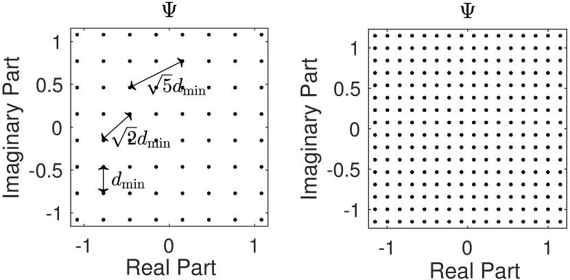
where $j$ is the index of the pass²²2Generally, the Spinal codes are transmitted pass by pass. The $j$ -th pass of Spinal codes consists of $n/k$ coded symbols $\{x_{1,j},\cdots,x_{n/k,j}\}$ . See Fig. 1 for the definition of a pass. . Fig. 2 illustrates two QAM modulation examples of the constellation mapping set $\Psi$ .

II-B ML Decoding of Spinal Codes

We consider ML decoding for Spinal codes in this correspondence. We denote $x_{i,j}(\mathbf{M})$ as the $j$ -th pass symbol generated by $\mathbf{s}_{i}$ from $\mathbf{M}$ . The received symbol at the receiver is denoted by $y_{i,j}=\alpha_{i,j}\cdot x_{i,j}(\mathbf{M})+n_{i,j}$ , where $\alpha_{i,j}\in\mathbb{C}$ is the fading coefficient and $n_{i,j}$ is the AWGN, with $n_{i,j}\sim\mathcal{CN}(0,\sigma^{2})$ . We denote $L$ as the transmitted passes, and $\mathbf{M}^{\star}\in\{0,1\}^{n}$ as the output from the ML decoder. With the above notations, the ML decoding rule is given by

\mathbf{M}^{\star}=\mathop{\arg\min}_{\mathbf{M}^{\prime}\in\left\{0,1\right\}^{n}}\sum_{i=1}^{n/k}\sum_{j=1}^{L}({y}_{i,j}-{{x}}_{i,j}(\mathbf{{M}}^{\prime}))^{2}.

(3)

III Error Floor and SNR Threshold Analysis

III-A Error Floor Analysis of Spinal Codes

The error floor analysis is based on the BLER analysis in the FBL regime in [32]. We find that the BLER does not drop to zero, regardless of how small the AWGN variance $\sigma^{2}$ becomes. In the following analysis, we first revisit the FBL BLER analysis presented in Lemma 1, and subsequently, we present our main results concerning the error floor of Spinal codes in Theorem 1.

Lemma 1.

(Restatement of [32, Theorem 2]) Consider $(n,k,c,\Psi,L)$ ³³3For short-hand notations, we call Spinal codes with message length $n$ , segmentation length $k$ , modulation order $c$ , channel input set $\Psi$ , and transmitted passes $L$ as $(n,k,c,\Psi,L)$ Spinal codes. Spinal codes transmitted over a complex fading channel with AWGN variance $\sigma^{2}$ , the average BLER given perfect CSI under ML decoding for Spinal codes can be approximated by a tight upper bound

{\color[rgb]{0,0,0}\definecolor[named]{pgfstrokecolor}{rgb}{0,0,0}\pgfsys@color@gray@stroke{0}\pgfsys@color@gray@fill{0}P_{e}\leq 1-\prod_{a=1}^{n/k}\left(1-\mathrm{min}\left\{1,\left(2^{k}-1\right)2^{n-ak}\cdot\mathscr{F}\left(L_{a},\sigma\right)\right\}\right),}

(4)

with $\mathscr{F}\left(L_{a},\sigma\right)$ equals to

\sum_{t=1}^{N}b_{t}\left(2^{-2c}\underbrace{\sum_{\beta_{i},\beta_{j}\in\Psi}\mathbb{E}_{H}\left[\exp\left\{\frac{-{|H(\beta_{i}-\beta_{j})|}^{2}}{4\sigma^{2}\mathrm{sin}^{2}\theta_{t}}\right\}\right]}_{G(\Psi,\sigma^{2},\theta_{t},f_{H}(h))}\right)^{L_{a}},

(5)

where $b_{t}=\frac{\theta_{t}-\theta_{t-1}}{\pi}$ , $\theta_{t}$ is arbitrarily chosen with $\theta_{0}=0$ , $\theta_{N}=\frac{\pi}{2}$ and $\theta_{0}<\theta_{1}<\cdots<\theta_{N}$ , $N$ represents the number of $\theta$ values which enables the adjustment of accuracy, $L_{a}=L(n/k-a+1)$ , and $H\in\mathbb{C}$ characterizes the random channel fading coefficient. The summation is taken over all constellation points $\beta_{i}$ and $\beta_{j}$ in the channel input set $\Psi$ .

Our error floor analysis is rooted in the key observation that $\mathscr{F}(L_{a},0)>0$ . As a result, the error probability remains non-zero, regardless of the SNR reaching infinity. Lemma 2 provides a mathematical demonstration of this phenomenon.

Lemma 2.

$\mathscr{F}(L_{a},\sigma)$ is monotonically increasing in terms of $\sigma\geq 0$ , with the minimum value $\mathscr{F}(L_{a},0)$ calculated by

\mathscr{F}(L_{a},0)=2^{-L_{a}c-1}.

(6)

Proof.

See Appendix A. ∎

The error floor observed in Spinal codes stems from their random coding structure. This randomness can cause collisions, where different seeds, $\mathbf{s}_{i}$ and $\mathbf{s}_{i}^{\prime}$ , produce identical outputs, leading to $\beta_{i}=\beta_{j}$ as illustrated in (13). Crucially, these collisions are an intrinsic feature of the random coding mechanism in Spinal codes and cannot be resolved by merely increasing the SNR.

Theorem 1.

A $(n,k,c,\Psi,L)$ Spinal codes will suffer from an error floor $P_{EF}$ , which is calculated by

P_{EF}=1-\prod_{a=1}^{n/k}\left(1-\mathrm{min}\left\{1,\left(2^{k}-1\right)2^{n-ak-L_{a}c-1}\right\}\right).

(7)

Proof.

Lemma 2 establishes that the function $\mathscr{F}(L_{a},\sigma)$ is bounded below by $2^{-L_{a}c-1}$ . This lower bound is attained when $\sigma=0$ , corresponding to the case where $\text{SNR}\rightarrow\infty$ . Therefore, applying Lemma 2 in Lemma 1 yields the expression for the error floor of Spinal codes. ∎

III-B SNR Threshold of the Error Floor

Our error floor analysis indicates that Spinal codes experience an error floor, where additional increases in SNR fail to lower the BLER. In practical applications, estimating the SNR threshold is crucial for efficient power allocation in Spinal codes. To address this need, we propose a method to approximate the SNR threshold for Spinal codes under QAM modulation. The main findings are presented in Theorem 2.

Theorem 2.

For an $(n,k,c,\Psi,L)$ Spinal codes where $c$ is a even, if the SNR $\gamma$ goes beyond a threshold with $\gamma\geq\gamma^{\text{th}}$ , where $\gamma^{\text{th}}$ satisfies

4\cdot\mathbb{E}_{H}\left[\exp\left\{\frac{-{3|H|}^{2}\gamma^{\text{th}}}{2(2^{c}-1)}\right\}\right]\ll 1,

(8)

Then, the BLER of Spinal codes will suffer from an error floor.

Proof.

See Appendix B. ∎

With Theorem 2 as a basis, we proceed to derive the SNR threshold for nakagami-m, rayleigh, and AWGN channels. These closed-form expressions are achieved by tailoring the distribution of the fading coefficient $H$ and explicitly calculating $\mathbb{E}_{H}\left[\exp\left\{\frac{-{3|H|}^{2}\gamma^{\text{th}}}{2(2^{c}-1)}\right\}\right]$ .

Corollary 1.

(i) For nakagami-m fading channel with a normalized fading mean square $\Omega=1$ , the SNR threshold of the error floor is approximated by

\gamma^{\text{th}}{\color[rgb]{0,0,0}\definecolor[named]{pgfstrokecolor}{rgb}{0,0,0}\pgfsys@color@gray@stroke{0}\pgfsys@color@gray@fill{0}\approx}\frac{2m(2^{c}-1)}{3}\left({\color[rgb]{0,0,0}\definecolor[named]{pgfstrokecolor}{rgb}{0,0,0}\pgfsys@color@gray@stroke{0}\pgfsys@color@gray@fill{0}\left(\frac{4}{x}\right)}^{1/m}-1\right).

(9)

(ii) For rayleigh fading channel with $\Omega=1$ , the SNR threshold of the error floor is approximated by

\gamma^{\text{th}}{\color[rgb]{0,0,0}\definecolor[named]{pgfstrokecolor}{rgb}{0,0,0}\pgfsys@color@gray@stroke{0}\pgfsys@color@gray@fill{0}\approx}\frac{2(2^{c}-1)}{3}\left({\color[rgb]{0,0,0}\definecolor[named]{pgfstrokecolor}{rgb}{0,0,0}\pgfsys@color@gray@stroke{0}\pgfsys@color@gray@fill{0}\left(\frac{4}{x}\right)}-1\right).

(10)

(iii) For AWGN channel, the SNR threshold of the error floor is approximated by

\gamma^{\text{th}}{\color[rgb]{0,0,0}\definecolor[named]{pgfstrokecolor}{rgb}{0,0,0}\pgfsys@color@gray@stroke{0}\pgfsys@color@gray@fill{0}\approx}\frac{2(2^{c}-1)}{3}\ln{\color[rgb]{0,0,0}\definecolor[named]{pgfstrokecolor}{rgb}{0,0,0}\pgfsys@color@gray@stroke{0}\pgfsys@color@gray@fill{0}\left(\frac{4}{x}\right)}.

(11)

where $x\ll 1$ , which can be chosen flexibly to adjust the precision of the approximation.

Proof.

See Appendix C. ∎

IV Numerical Verification

Fig. 3 illustrate the error curves, error floor, and SNR thresholds over the AWGN, rayleigh, and nakagami-m fading channels with parameter $m=1.5$ , respectively.

IV-A Error Floor

From Fig. 3, we observe that Spinal codes exhibit a consistent error floor across various channel types. This consistency indicates that the error floor is primarily attributed to the inherent random coding structure and the potential for collisions⁴⁴4A collision occurs when distinct messages are encoded into the same codeword. For example, if $\mathbf{M}_{1}$ and $\mathbf{M}_{2}$ are two distinct messages such that their encoded codewords satisfy $\mathbf{X}=f(\mathbf{M}_{1})=f(\mathbf{M}_{2})$ , where $f(\cdot)$ is the encoding function, then a collision has occurred. In random coding schemes like Spinal codes, the codeword $\mathbf{X}$ is generated randomly, resulting in a non-zero probability of collision and thus the error floor. within Spinal codes, rather than to external channel characteristics. The orange horizontal dashed line in each graph, as predicted by Theorem 1, validates our theoretical analysis, demonstrating that the error floor is a fundamental limitation of Spinal codes, irrespective of the channel type.

Additionally, as depicted in Fig. 3, the error floor of Spinal codes decreases with an increase in both the modulation order $c$ and the number of transmitted passes $L$ , consistent with the predictions of Theorem 1. However, since Spinal codes are rateless, the number of transmitted passes $L$ continues to increase until successful decoding is achieved. Therefore, the modulation order parameter $c$ is an important variable that may guide balancing the trade-off between the error floor and the coding complexity of Spinal codes.

IV-B SNR Threshold

From Fig. 4, we observe that the predicted SNR thresholds, consistently mark the onset of the error floor across different types of fading channels and various parameter configurations. A comparative analysis of the first row of subfigures with the second reveals that the SNR thresholds are independent of the number of transmitted passes, $L$ , and predominantly influenced by the modulation order, $c$ , and the types of channels. This observation highlights the insight that, for Spinal codes, transmitting more passes of symbols can lower the error floor but does not affect the SNR threshold.

V Conclusion

In this correspondence, we studied the error floor in Spinal codes and determined that their random coding structure is the underlying cause. We derived explicit expressions for the error floor associated with Spinal codes and calculated approximate SNR thresholds under QAM modulation, indicating the onset of the error floor across rayleigh, nakagami-m, and AWGN channels. Our numerical results corroborated these findings. In addition, the analysis and numerical results revealed that, while transmitting additional passes of symbols can reduce the error floor, it cannot change the SNR threshold. This provides insights into the SNR working region and informs the design and transmission practices of codes.

Appendix A Proof of Lemma 2

Proof.

The monotonically increasing property is trivial. Our focus is on solving $\mathscr{F}(L_{a},0)$ , which is equivalent to addressing $G\left(\Psi,0,\theta_{t},f_{H}(h)\right)$ as specified in (5). To facilitate this, we first rewrite the function $G\left(\Psi,\sigma^{2},\theta_{t},f_{H}(h)\right)$ as

	$\displaystyle\underset{\begin{subarray}{c}\beta_{i},\beta_{j}\in\Psi\\ \beta_{i}=\beta_{j}\end{subarray}}{\sum}\mathbb{E}_{H}\left[\exp\left\{\frac{-{\|H(\beta_{i}-\beta_{j})\|}^{2}}{4\sigma^{2}\mathrm{sin}^{2}\theta_{t}}\right\}\right]+$		(12)
	$\displaystyle\underset{\begin{subarray}{c}\beta_{i},\beta_{j}\in\Psi\\ \beta_{i}\neq\beta_{j}\end{subarray}}{\sum}\mathbb{E}_{H}\left[\exp\left\{\frac{-{\|H(\beta_{i}-\beta_{j})\|}^{2}}{4\sigma^{2}\mathrm{sin}^{2}\theta_{t}}\right\}\right],$		(12)

where the first term satisfies

\underset{\begin{subarray}{c}\beta_{i},\beta_{j}\in\Psi\\ \beta_{i}=\beta_{j}\end{subarray}}{\sum}\mathbb{E}_{H}\left[\exp\left\{\frac{-{|H(\beta_{i}-\beta_{j})|}^{2}}{4\sigma^{2}\mathrm{sin}^{2}\theta_{t}}\right\}\right]=\underset{\begin{subarray}{c}\beta_{i},\beta_{j}\in\Psi\\ \beta_{i}=\beta_{j}\end{subarray}}{\sum}1=2^{c},

(13)

and the second term satisfies

\lim\limits_{\sigma\rightarrow 0}\underset{\begin{subarray}{c}\beta_{i},\beta_{j}\in\Psi\\ \beta_{i}\neq\beta_{j}\end{subarray}}{\sum}\mathbb{E}_{H}\left[\exp\left\{\frac{-{|H(\beta_{i}-\beta_{j})|}^{2}}{4\sigma^{2}\mathrm{sin}^{2}\theta_{t}}\right\}\right]=0.

(14)

As such, we have that $G\left(\Psi,0,\theta_{t},f_{H}(h)\right)=2^{c}$ . Applying it in (5) yields

\mathscr{F}\left(L_{a},0\right)=\sum_{t=1}^{N}b_{t}\cdot 2^{-cL_{a}}=2^{-L_{a}c-1}.

(15)

∎

Appendix B Proof of Theorem 2

Proof.

For QAM modulation with even modulation order $c$ , the average SNR can be calculated by

\gamma=\frac{(2^{c}-1)\cdot d_{\min}^{2}}{6\sigma^{2}},

(16)

where $d_{\min}$ is the minimum distance of the QAM symbols. Substituting (16) into $G(\Psi,\sigma^{2},\theta_{t},f_{H}(h))$ yields

\sum_{\beta_{i},\beta_{j}\in\Psi}\mathbb{E}_{H}\left[\exp\left\{\frac{-{3|H(\beta_{i}-\beta_{j})|}^{2}\gamma}{2(2^{c}-1)d_{\min}^{2}\mathrm{sin}^{2}\theta_{t}}\right\}\right].

(17)

On the other hand, the distance between a pair of QAM symbols forms a finite set, represented as $\mathcal{S}=\{|\beta_{i}-\beta_{j}|:\beta_{i},\beta_{j}\in\Psi\}$ . From Fig. 2, we can numerate the above set as $\mathcal{S}=\{0,d_{\min},\sqrt{2}d_{\min},2d_{\min},\cdots,\sqrt{2}(2^{c/2}-1)d_{\min}\}$ . With set $\mathcal{S}$ , we can rewrite (17) as

		$\displaystyle\sum_{d\in\mathcal{S}}\underset{\begin{subarray}{c}\beta_{i},\beta_{j}\in\Psi\\ \|\beta_{i}-\beta_{j}\|=d\end{subarray}}{\sum}\mathbb{E}_{H}\left[\exp\left\{\frac{-{3\|H(\beta_{i}-\beta_{j})\|}^{2}\gamma}{2(2^{c}-1)d_{\min}^{2}\mathrm{sin}^{2}\theta_{t}}\right\}\right]$		(18)
		$\displaystyle=\sum_{d\in\mathcal{S}}A_{d}\mathbb{E}_{H}\left[\exp\left\{\frac{-{3\|H\|}^{2}d^{2}\gamma}{2(2^{c}-1)d_{\min}^{2}\mathrm{sin}^{2}\theta_{t}}\right\}\right],$		(18)

where $A_{d}$ is the number of element pairs $(\beta_{i},\beta_{j})$ within $\Psi$ that are exactly $d$ units apart, with

A_{d}=|\{(\beta_{i},\beta_{j}):|\beta_{i}-\beta_{j}|=d,\beta_{i},\beta_{j}\in\Psi\}|.

(19)

Denote $g(d,\gamma)=\mathbb{E}_{H}\left[\exp\left\{\frac{-{3|H|}^{2}d^{2}\gamma}{2(2^{c}-1)d_{\min}^{2}\mathrm{sin}^{2}\theta_{t}}\right\}\right]$ , and (18) is reduced to $\sum_{d\in\mathcal{S}}A_{d}g(d,\gamma)$ , which can be expanded by:

A_{0}+A_{d_{\min}}g(d_{\min},\gamma)+A_{\sqrt{2}d_{\min}}g(\sqrt{2}d_{\min},\gamma)\cdots.

(20)

Because $g(nd,\gamma)=g(d,\gamma)^{n^{2}}$ and $g(d,\gamma)\ll 1$ under high SNR $\gamma$ , the tail of (20) is a higher-order infinitesimal relative to $g(d_{\min},\gamma)$ . Therefore, (20) is simplified as

A_{0}+A_{d_{\min}}g(d_{\min},\gamma)+o(g(d_{\min},\gamma)).

(21)

From the proof of Lemma 2, we know that

\lim_{\gamma\rightarrow\infty}A_{0}+A_{d_{\min}}g(d_{\min},\gamma)+o(g(d_{\min},\gamma))=A_{0},

(22)

Thus, the SNR threshold can be approximated by $\gamma^{\text{th}}$ , such that $A_{d_{\min}}g(d_{\min},\gamma^{\text{th}})\ll A_{0}$ , or equivalently,

\frac{A_{d_{\min}}g(d_{\min},\gamma^{\text{th}})}{A_{0}}\ll 1.

(23)

Note that $A_{0}=2^{c}$ and $A_{d_{\min}}\approx 4\cdot 2^{c}$ , substituting $g(d_{\min},\gamma^{\text{th}})=\mathbb{E}_{H}\left[\exp\left\{\frac{-{3|H|}^{2}\gamma^{\text{th}}}{2(2^{c}-1)\mathrm{sin}^{2}\theta_{t}}\right\}\right]$ into (23) yields

4\cdot\mathbb{E}_{H}\left[\exp\left\{\frac{-{3|H|}^{2}\gamma^{\text{th}}}{2(2^{c}-1)\mathrm{sin}^{2}\theta_{t}}\right\}\right]\ll 1.

(24)

Without loss of generality, setting $\theta=\pi/2$ allows us to impose a stricter condition, thus completing the proof. ∎

Appendix C Proof of Corollary 1

Proof.

The expectation on the left-hand side of (8) over different channels are:

(i) Nakagami-m: In this case, the Probability Density Function (PDF) of the modulus of $\alpha_{i,j}$ is $f_{|H|}(r)=\frac{2m^{m}}{\Gamma(m)}\cdot r^{2m-1}\cdot\exp\{{-mr^{2}}\}$ . Substituting it into the expectation yields:

		$\displaystyle\mathbb{E}_{H}\left[\exp\left\{\frac{-{3\|H\|}^{2}\gamma^{\text{th}}}{2(2^{c}-1)}\right\}\right]=\mathbb{E}_{\|H\|}\left[\exp\left\{\frac{-{3\|H\|}^{2}\gamma^{\text{th}}}{2(2^{c}-1)}\right\}\right]$		(25)
		$\displaystyle=\int_{0}^{\infty}\exp\left\{\frac{-{3r}^{2}\gamma^{\text{th}}}{2(2^{c}-1)}\right\}\cdot\frac{2m^{m}r^{2m-1}}{\Gamma(m)}\exp\left\{{-mr^{2}}\right\}\mathrm{d}r.$		(25)

By implementing the substitution $q=\left(\frac{{3}\gamma^{\text{th}}}{2(2^{c}-1)}+m\right)r^{2}$ , the above improper integral turns to:

		$\displaystyle\frac{m^{m}}{\left(\frac{{3}\gamma^{\text{th}}}{2(2^{c}-1)}+m\right)^{m}\Gamma(m)}\underbrace{\int_{0}^{\infty}e^{-q}\cdot q^{m-1}}_{\Gamma(m)}\mathrm{d}q$		(26)
		$\displaystyle=\left(\frac{2m(2^{c}-1)}{3\gamma^{\text{th}}+2m(2^{c}-1)}\right)^{m}.$		(26)

(ii) Rayleigh: In this case, the PDF of the modulus of $\alpha_{i,j}$ is $f_{|H|}(r)=2r\cdot\exp\{-r^{2}\}$ . We have:

		$\displaystyle\mathbb{E}_{H}\left[\exp\left\{\frac{-{3\|H\|}^{2}\gamma^{\text{th}}}{2(2^{c}-1)}\right\}\right]=\mathbb{E}_{\|H\|}\left[\exp\left\{\frac{-{3\|H\|}^{2}\gamma^{\text{th}}}{2(2^{c}-1)}\right\}\right]$		(27)
		$\displaystyle=\int_{0}^{\infty}\exp\left\{\frac{-{3r}^{2}\gamma^{\text{th}}}{2(2^{c}-1)}\right\}\cdot{2r}\cdot\exp\{-r^{2}\}~{}\mathrm{d}r.$		(27)

By implementing the substitution $q=\left(\frac{{3}\gamma^{\text{th}}}{2(2^{c}-1)}+1\right)r^{2}$ , the above improper integral turns to:

\color[rgb]{0,0,0}\definecolor[named]{pgfstrokecolor}{rgb}{0,0,0}\pgfsys@color@gray@stroke{0}\pgfsys@color@gray@fill{0}\frac{1}{\frac{{3}\gamma^{\text{th}}}{2(2^{c}-1)}+1}\int_{0}^{\infty}e^{-q}\mathrm{d}q=\frac{2(2^{c}-1)}{3\gamma^{\text{th}}+2(2^{c}-1)}.

(28)

(iii) AWGN: In this case, $|H|\equiv 1$ holds, and we have:

\displaystyle\mathbb{E}_{H}\left[\exp\left\{\frac{-{3|H|}^{2}\gamma^{\text{th}}}{2(2^{c}-1)}\right\}\right]=\exp\left\{\frac{-{3}\gamma^{\text{th}}}{2(2^{c}-1)}\right\}.

(29)

Then, by setting the left-hand side of (8) as $x$ and explicitly solving $\gamma^{\text{th}}$ , we can obtain the threshold $\gamma^{\text{th}}$ over the nagakami-m, rayleigh, and AWGN channel, respectively. ∎

References

[1] J. Perry, H. Balakrishnan, and D. Shah, “Rateless spinal codes,” Proc. ACM HotNets, pp. 1–6, 2011.
[2] H. Balakrishnan, P. Iannucci, J. Perry, and D. Shah, “De-randomizing shannon: The design and analysis of a capacity-achieving rateless code,” arXiv preprint arXiv:1206.0418, 2012.
[3] A. Shokrollahi, “Raptor codes,” IEEE Trans. Inf. Theory, vol. 52, no. 6, pp. 2551–2567, 2006.
[4] A. Gudipati and S. Katti, “Strider: Automatic rate adaptation and collision handling,” Proc. ACM SIGCOMM 2011, pp. 158–169, 2011.
[5] R. Gallager, “Low-density parity-check codes,” IRE Trans. Inf. Theory, vol. 8, no. 1, pp. 21–28, 1962.
[6] J. Perry, P. A. Iannucci, K. E. Fleming, H. Balakrishnan, and D. Shah, “Spinal codes,” Proc. ACM SIGCOMM 2012, pp. 49–60, 2012.
[7] X. Yu, Y. Li, W. Yang, and Y. Sun, “Design and analysis of unequal error protection rateless Spinal codes,” IEEE Trans. Commun., vol. 64, no. 11, pp. 4461–4473, 2016.
[8] W. Yang, Y. Li, X. Yu, and Y. Sun, “Two-way spinal codes,” in Proc. IEEE ISIT, 2016, pp. 1919–1923.
[9] Y. Li, J. Wu, B. Tan, M. Wang, and W. Zhang, “Compressive spinal codes,” IEEE Trans. Veh. Technol., vol. 68, no. 12, pp. 11 944–11 954, 2019.
[10] A. Li, S. Wu, J. Jiao, N. Zhang, and Q. Zhang, “Spinal codes over fading channel: Error probability analysis and encoding structure improvement,” IEEE Trans. Wirel. Commun., vol. 20, no. 12, pp. 8288–8300, 2021.
[11] Y. Hu, R. Liu, H. Bian, and D. Lyu, “Design and analysis of a low-complexity decoding algorithm for spinal codes,” IEEE Trans. Veh. Technol., vol. 68, no. 5, pp. 4667–4679, 2019.
[12] W. Yang, Y. Li, X. Yu, and J. Li, “A low complexity sequential decoding algorithm for rateless spinal codes,” IEEE Commun. Lett., vol. 19, no. 7, pp. 1105–1108, 2015.
[13] H. Bian, R. Liu, A. Kaushik, and R. Duan, “Segmented crc-aided spinal codes with a novel sliding window decoding algorithm,” in Proc. IEEE IWCMC 2019, pp. 1539–1543.
[14] Z. Zhang, L. Zhao, and J. Bai, “A decoding algorithm for spinal codes over fading channel,” in ACM Proc. ICCIP, 2023, pp. 415–419.
[15] X. Wen, Q. Li, H. Mao, Y. Luo, B. Yan, and F. Huang, “Novel reconciliation protocol based on spinal code for continuous-variable quantum key distribution,” Quantum Inf. Process., vol. 19, no. 9, p. 350, 2020.
[16] J. Xu, S. Wu, J. Jiao, and Q. Zhang, “Optimized puncturing for the spinal codes,” in Proc. IEEE ICC, 2019, pp. 1–5.
[17] A. Li, S. Wu, Y. Wang, J. Jiao, and Q. Zhang, “Spinal codes over BSC: Error probability analysis and the puncturing design,” in Proc. IEEE VTC2020-Spring, 2020, pp. 1–5.
[18] S. Meng, S. Wu, A. Li, J. Jiao, N. Zhang, and Q. Zhang, “Analysis and optimization of the harq-based spinal coded timely status update system,” IEEE Trans. Commun., vol. 70, no. 10, pp. 6425–6440, 2022.
[19] X. Xu, S. Wu, D. Dong, J. Jiao, and Q. Zhang, “High performance short polar codes: A concatenation scheme using spinal codes as the outer code,” IEEE Access, vol. 6, pp. 70 644–70 654, 2018.
[20] H. Liang, A. Liu, X. Tong, and C. Gong, “Raptor-like rateless spinal codes using outer systematic polar codes for reliable deep space communications,” in IEEE INFOCOM Workshops, 2020, pp. 1045–1050.
[21] D. Dong, S. Wu, X. Jiang, J. Jiao, and Q. Zhang, “Towards high performance short polar codes: concatenated with the spinal codes,” in Proc. IEEE PIMRC, 2017, pp. 1–5.
[22] Y. Cao, F. Du, J. Zhang, and X. Peng, “Polar-UEP spinal concatenated encoding in free-space optical communication,” Applied Optics, vol. 61, no. 1, pp. 273–278, 2022.
[23] M. Vaezi, A. Azari, S. R. Khosravirad, M. Shirvanimoghaddam, M. M. Azari, D. Chasaki, and P. Popovski, “Cellular, wide-area, and non-terrestrial IoT: A survey on 5G advances and the road toward 6G,” IEEE Commun. Surv. Tutorials, vol. 24, no. 2, pp. 1117–1174, 2022.
[24] L. Wang, Y. L. Che, J. Long, L. Duan, and K. Wu, “Multiple access mmWave design for UAV-aided 5G communications,” IEEE Wirel. Commun., vol. 26, no. 1, pp. 64–71, 2019.
[25] X. Pang, M. Liu, Z. Li, Z. Jiao, and S. Sun, “Trust function based spinal codes over the mobile fading channel between UAVs,” in Proc. IEEE GLOBECOM, 2018, pp. 1–7.
[26] S. Wu, D. Li, J. Jiao, and Q. Zhang, “CS-LTP-Spinal: A cross-layer optimized rate-adaptive image transmission system for deep-space exploration,” Sci. China Inf. Sci., vol. 65, no. 1, p. 112303, 2022.
[27] H. Bian, R. Liu, X. Shi, and J. Thompson, “A high-throughput fine-grained rate adaptive transmission scheme for a LEO satellite communication system,” in NASA/ESA Conference on Adaptive Hardware and Systems (AHS). IEEE, 2018, pp. 192–197.
[28] P. A. Iannucci, J. Perry, H. Balakrishnan, and D. Shah, “No symbol left behind: A link-layer protocol for rateless codes,” in Proc. ACM Mobicom, 2012, pp. 17–28.
[29] W. Yang, Y. Li, and X. Yu, “Performance of spinal codes with sliding window decoding,” in IEEE Proc. ISIT, 2017, pp. 2203–2207.
[30] A. Li, S. Wu, X. Chen, and S. Sun, “Tight upper bounds on the BLER of Spinal codes over the AWGN channel,” IEEE Trans. Commun. (Early Access), 2024.
[31] X. Chen, A. Li, and S. Wu, “Tight upper bounds on the error probability of spinal codes over fading channels,” in Proc. IEEE ISIT, 2023, pp. 1277–1282.
[32] A. Li, X. Chen, S. Wu, G. C.F., Lee, and S. Sun, “A unified expression for upper bounds on the BLER of spinal codes over fading channels,” submitted to IEEE Trans. Wirel. Commun., arXiv preprint arXiv:2407.03741, 2024.
[33] M. Mondelli, S. H. Hassani, and R. L. Urbanke, “Unified Scaling of Polar Codes: Error Exponent, Scaling Exponent, Moderate Deviations, and Error Floors,” IEEE Trans. Inf. Theory, vol. 62, no. 12, pp. 6698–6712, 2016.
[34] A. Eslami and H. Pishro-Nik, “On finite-length performance of polar codes: Stopping sets, error floor, and concatenated design,” IEEE Trans. Commun., vol. 61, no. 3, pp. 919–929, 2013.
[35] H. Ju, J. Park, M. Y. Chung, and S. Kim, “Lowering the error-floor of CRC-concatenated Polar codes with improved partial protection,” in 94th IEEE Vehicular Technology Conference, VTC Fall 2021, Norman, OK, USA, September 27-30, 2021. IEEE, 2021, pp. 1–6.
[36] E. Psota, J. Kowalczuk, and L. C. Pérez, “A deviation-based conditional upper bound on the error floor performance for min-sum decoding of short LDPC codes,” IEEE Trans. Commun., vol. 60, no. 12, pp. 3567–3578, 2012.
[37] R. Asvadi, A. H. Banihashemi, and M. Ahmadian-Attari, “Lowering the error floor of LDPC codes using cyclic liftings,” IEEE Trans. Inf. Theory, vol. 57, no. 4, pp. 2213–2224, 2011.
[38] P. Neshaastegaran, A. H. Banihashemi, and R. H. Gohary, “Error floor estimation of LDPC coded modulation systems using importance sampling,” IEEE Trans. Commun., vol. 69, no. 5, pp. 2784–2799, 2021.
[39] X. Tao, X. Chen, and B. Wang, “On the construction of QC-LDPC codes based on integer sequence with low error floor,” IEEE Commun. Lett., vol. 26, no. 10, pp. 2267–2271, 2022.