Error analysis for parabolic optimal control problems with measure data in a nonconvex polygonal domain

Pratibha Shakya Department of Mathematics, Indian Institute of Technology Delhi, New Delhi, 110016 [email protected]

Abstract.

This paper considers the finite element approximation to parabolic optimal control problems with measure data in a nonconvex polygonal domain. Such problems usually possess low regularity in the state variable due to the presence of measure data and the nonconvex nature of the domain. The low regularity of the solution allows the finite element approximations to converge at lower orders. We prove the existence, uniqueness and regularity results for the solution to the control problem satisfying the first order optimality condition. For our error analysis we have used piecewise linear elements for the approximation of the state and co-state variables, whereas piecewise constant functions are employed to approximate the control variable. The temporal discretization is based on the implicit Euler scheme. We derive both a priori and a posteriori error bounds for the state, control and co-state variables. Numerical experiments are performed to validate the theoretical rates of convergence.

Mathematics subject classification: 49J20, 49K20, 65N15, 65N30.

Key words. A priori and a posteriori error estimates, finite element method, measure data, nonconvex polygonal domain, optimal control problem.

1. Introduction

The aim of this paper is to study both a priori and a posteriori error analysis of finite element approximations to the following model control problem:

(1.1)

\displaystyle\min_{u\in U_{ad}}J(y,u),

where $J(y,u):=\frac{1}{2}\int_{0}^{T}\|y-y_{d}\|_{L^{2}(\Omega)}^{2}\,dt+\frac{\Lambda}{2}\int_{0}^{T}\|u\|_{L^{2}(\Omega)}\,dt$ with $u$ represents the control variable and $y$ indicates the associated state variable. The state equation is given by

(1.2)

\displaystyle\begin{cases}\frac{\partial y}{\partial t}-\Delta y=\sigma\tau+u\;\;\;\text{in}\;\Omega_{T},\\ y=0\;\;\;\;\text{on}\;\Gamma_{T},\\ y(\cdot,0)=y_{0}\;\;\;\;\text{in}\;\Omega.\end{cases}

In the above, $\Omega$ is a nonconvex polygonal domain in $\mathbb{R}^{2}$ with Lipschitz boundary $\partial\Omega$ . Set $\Omega_{T}=\Omega\times(0,T]$ and $\Gamma_{T}=\partial\Omega\times(0,T]$ . The boundary $\partial\Omega$ can be expressed as $\partial\Omega=\displaystyle\cup_{j=1}^{m}\Gamma_{j}$ with $\Gamma_{j}$ , $j=1,2,\ldots,m$ , are edges of the polygon. The constraints on the control variable are specified through the closed and convex subset of $L^{2}(0,T;L^{2}(\Omega))$ as follows:

(1.3)

\displaystyle U_{ad}:=\{u\in L^{2}(0,T;L^{2}(\Omega)):u_{a}\leq u(x,t)\leq u_{b}\;\text{for a. a.}\;(x,t)\in\Omega_{T}\}.

Assume that the given functions $y_{0}\in L^{2}(\Omega),\;y_{d}\in H^{1}(0,T;L^{2}(\Omega)),\;\sigma\in\mathcal{C}([0,T];L^{2}(\Omega))$ and $\tau\in\mathfrak{B}[0,T]$ , where $\mathfrak{B}[0,T]$ is the space of real and regular Borel measures in $[0,T]$ . Further, the constants $u_{a},\,u_{b}\in\mathbb{R}$ satisfy $u_{a}<u_{b}$ , the regularization parameter $\Lambda>0$ and the final time $T<\infty$ .

Optimal control problems are widely used in scientific and engineering applications [26, 36]. The numerical study of such type of problems began in early 1970s [16, 17]. Thereafter there have been several notable contributions to this discipline and it is impossible to list all of them. Nevertheless, for the development of the finite element approach for parabolic optimal control problems (POCPs), see [19, 23, 32, 37, 42] and references therein. The authors of [33, 34] have utilized discontinuous Galerkin technique for temporal discretization and established convergence results for space-time finite element discretizations for POCPs. In [35], the authors have adopted Petrov Galerkin Crank-Nicolson method for discretization of the control problem and derived related error estimates. The sparse POCPs have been analyzed by the authors of [11], where the control variable is taken to be an element of the measure space. They have provided a priori error estimates for the control problem.

Following the work of Babuška and Rheinboldt [4], the adaptive finite element method has grown popularity in scientific computing. It is well known that a posteriori error estimation is a necessary part of adaptivity for mesh refinement. The pioneer work has been made by Liu and Yan [28] for residual based a posteriori error estimates, Becker et al. [7] for dual-weighted goal oriented adaptivity and Li et al. [25] for recovery type a posteriori error estimators. A posteriori error analysis for optimal control problems governed by parabolic equation have been extensively investigated by numerous authors in [29, 31, 43, 40, 41].

POCPs are widely encountered in mathematical models representing groundwater contamination transmission, environmental modeling, petroleum reservoir simulation, and a variety of other applications. There are several real-world applications for POCPs when the state variable possesses less regularity due to the support of the source. Essentially, the support for the source function must be relatively tiny in comparison to the real size of the domain $\Omega$ . This feature drives us to explore control problems in which the source functions are measure data (elements from $\mathcal{M}(\Omega)$ ). The POCPs with measure data encounter environmental concerns such as air pollution and waste-water treatment. Due to the presence of measure data, the solution of the state variable possesses less regularity which makes finite element error analysis more challenging. Therefore, an attempt has been made to study the convergence properties of the finite element method for such problems.

The study of optimal control problems governed by partial differential equations over a nonsmooth domain is a difficult task. The existence of re-entrant corners in the domain causes both theoretical and numerical analysis to be complicated. However, although there is a significant amount of research on the numerical analysis of the elliptic problem with a nonconvex domain [3, 5, 6, 20, 21] and quite a few works on the parabolic problem [12, 13]. For optimal control problems, there was not much work done in the nonconvex polygonal domain. In recently published article [2], Apel et al. developed a priori error estimates for the optimal control problem on a nonconvex domain.

The numerical analysis of the problem under consideration is difficult because of the presence of measure data and the nonconvex nature of the domain. The low regularity of the solution allows the numerical approximations to converge at lower orders. This study aims to look at the finite element approximation and mathematical formulation of the model problem. The results regarding the existence and uniqueness of the solution to the control problem are proved. Based on the necessary optimality condition, the regularity results for the control problem are explored. For the control variable, piecewise constant functions are utilized, whereas piecewise linear and continuous functions are used to approximate the state and co-state variables. The backward-Euler technique is used for temporal discretization. We studied completely discrete finite element approximations of the POCP (1.1)-(1.3) and established both a priori and a posteriori error bounds for the state, co-state and control variables.

We mention [8, 9] for a great introduction to nonlinear parabolic equations with measure data. The author of [10] have addressed the semilinear parabolic problems with measure data. Additionally, the asymptotic behavior of a parabolic equation involving measure data has been studied by Gong in [18]. For recent research on POCPs with measure data, we refer to [38, 39].

The paper is structured as follows: We introduce some function spaces and preliminary material in Section $2$ . We discuss the weak formulation and investigate the existence, uniqueness and regularity results of the solution to the control problem (1.1)-(1.3). The convergence analysis for the a priori error estimates of the space-time finite element approximation to the control problem is discussed in Section 4. In Section 5, we derived a posteriori error estimates for the control problem. In the last section, we perform numerical experiments to demonstrate the theoretical findings.

2. Notation and wellposedness

This section introduces some function spaces to be used in our analysis. It also contains the existence, uniqueness, and regularity results of the solutions to the POCP (1.1)-(1.3).

For bounded polygonal domain $\Omega$ , let the inner angles of corners of the domain be denoted by $\omega_{j}$ . Set $\beta=\displaystyle\max_{j}\frac{\pi}{\omega_{j}}\in(\frac{1}{2},1)$ . For simplicity, it is assumed that there is only one re-entrant corner with angle $\omega$ such that $\pi<\omega<2\pi$ . For example, the interior angle for $L$ -shape domain $\omega=\frac{3\pi}{2}$ , and hence $\beta=\frac{2}{3}<1$ . Let $\mathcal{C}(\overline{\Omega})$ denote the space of continuous functions defined on $\overline{\Omega}$ . The space $W^{m,p}(\Omega)$ indicates the usual Sobolev spaces [1] with norm $\|\cdot\|_{W^{m,p}(\Omega)}$ and semi-norm $|\cdot|_{W^{m,p}(\Omega)}$ . Define $W_{0}^{m.p}(\Omega):=\{v\in W^{m,p}(\Omega):v=0\;\;\text{on}\;\;\partial\Omega\}$ . For $p=2$ , the spaces $W^{m,p}(\Omega)$ and $W^{m,p}_{0}(\Omega)$ are represented by $H^{m}(\Omega)$ and $H^{m}_{0}(\Omega)$ , respectively with norm $\|\cdot\|_{H^{m}(\Omega)}$ and semi-norm $|\cdot|_{H^{m}(\Omega)}$ . In particular, for $0<s<1$ and $1<p\leq\infty$ , the norm on the fractional order Sobolev space $W^{s,p}(\Omega)$ is given by

\displaystyle\|v\|_{W^{s,p}(\Omega)}=\Big{(}\|v\|_{L^{p}(\Omega)}^{p}+\int_{\Omega}\int_{\Omega}\frac{|v(x)-v(y)|^{p}}{|x-y|^{2+ps}}\,dxdy\Big{)}^{\frac{1}{p}}.

Set $H^{m,m^{\prime}}(\Omega_{T})=L^{2}(0,T;H^{m}(\Omega))\cap H^{m^{\prime}}(0,T;L^{2}(\Omega))$ with the standard norm

\displaystyle\|w\|_{H^{m,m^{\prime}}(\Omega_{T})}:=\Big{(}\int_{0}^{T}\|w(\cdot,t)\|^{2}_{H^{m}(\Omega)}\,dt+\int_{\Omega}\|w(x,\cdot)\|^{2}_{H^{m^{\prime}}([0,T])}\,dx\Big{)}^{\frac{1}{2}},

where $\|\cdot\|_{H^{m^{\prime}}([0,T])}$ denote the norm on $H^{m^{\prime}}([0,T])$ .

Further, let $\mathcal{X}(0,T),\;\mathcal{\hat{X}}(0,T)$ and $W(0,T)$ denote $L^{2}(0,T;H^{1}_{0}(\Omega))\cap H^{1}(0,T;H^{-1}(\Omega))$ ,
$L^{2}(0,T;H^{1+s}(\Omega)\cap H^{1}_{0}(\Omega))\cap H^{1}(0,T;L^{2}(\Omega))$ and $L^{2}(0,T;H^{1}_{0}(\Omega))\cap L^{\infty}(0,T;L^{2}(\Omega))$ , respectively for $s\in(\frac{1}{2},\beta)$ . The symbols $(\cdot,\cdot)$ and $(\cdot,\cdot)_{\Omega_{T}}$ denote the $L^{2}$ -inner product on $L^{2}(\Omega)$ and $L^{2}(0,T;L^{2}(\Omega))$ , respectively. Hereafter $C$ denotes a positive generic constant which is independent of the mesh parameters $h$ and $k$ , which may depend on final time $T$ .

We employ the transposition approach developed by Lions and Magenes (cf. [27]) to assertion that the state equation (1.2) has a unique solution. The weak form of (1.2) is stated as: Find $y\in W(0,T)$ such that

(2.1)

-(y,\frac{\partial w}{\partial t})_{\Omega_{T}}+(\nabla y,\nabla w)_{\Omega_{T}}=\langle\sigma\tau,w\rangle_{\Omega_{T}}+(u,w)_{\Omega_{T}}+(y_{0},w(\cdot,0))\;\;\forall w\in\mathcal{X}(0,T),

where we utilized $w(\cdot,T)=0$ and $\langle\sigma\tau,w\rangle_{\Omega_{T}}$ is defined as

\langle\sigma\tau,w\rangle_{\Omega_{T}}=\int_{0}^{T}\int_{\Omega}\sigma(x,t)w(x,t)\,dx\,d\tau(t)\;\;\;\;\forall w\in\mathcal{C}([0,T];L^{2}(\Omega)).

In the subsequent theorem, we provide a priori bounds for the state variable which are essential to our analysis. For a proof, see [39].

Theorem 2.1.

For $u\in L^{2}(0,T;L^{2}(\Omega))\cap L^{\infty}(0,T;L^{2}(\Omega))$ , assume that the given functions $\sigma\in\mathcal{C}([0,T];L^{2}(\Omega))$ , $\tau\in\mathfrak{B}[0,T]$ and $y_{0}\in L^{2}(\Omega)$ . Then, the unique solution $y\in W(0,T)$ of the problem (1.2) exists and satisfies a priori bound:

\displaystyle\|y\|_{L^{2}(0,T;H^{1}_{0}(\Omega))}+\|y\|_{L^{\infty}(0,T;L^{2}(\Omega))}\leq C\Big{(}\|\sigma\|_{L^{\infty}(0,T;L^{2}(\Omega))}\|\tau\|_{\mathfrak{B}[0,T]}+\|u\|_{L^{2}(0,T;L^{2}(\Omega))}+\|y_{0}\|_{L^{2}(\Omega)}\Big{)}.

The weak formulation of the control problem (1.1)-(1.3) is as follows:

(2.2)

\displaystyle\begin{cases}\displaystyle\min_{u\in U_{ad}}J(y,u)\\ -(y,\frac{\partial w}{\partial t})_{\Omega_{T}}+(\nabla y,\nabla w)_{\Omega_{T}}=\langle\sigma\tau,w\rangle_{\Omega_{T}}+(u,w)_{\Omega_{T}}+(y_{0},w(\cdot,0))\;\;\forall w\in\mathcal{X}(0,T),\end{cases}

where $w(\cdot,T)=0$ and $\langle\sigma\tau,w\rangle_{\Omega_{T}}$ is defined as before.

From the standard arguments, there exists a unique solution $(y,u)$ for the problem (2.2). Let $\mathcal{J}(u):=J(y(u),u)$ denote the reduced cost functional, where for each $u\in L^{2}(0,T;L^{2}(\Omega))$ the state $y(u)$ is the weak solution of (2.1). It should be noted that the cost functional of the optimal control problem (2.2) is strictly convex and hence, in light of the Theorem 2.1, it is bounded. This ensures the existence of an optimal solution. Since $\mathcal{J}$ is twice Fréchet differentiable convex function and $U_{ad}$ is a closed convex subset of $L^{2}(0,T;L^{2}(\Omega))$ , the existence of unique control is guaranteed. For further reading, we refer to [30].

We now state the first-order optimality condition which is necessary and sufficient for the optimal control problem (2.2).

Lemma 2.2.

The optimal control problem (2.2) has a unique solution $(y,u)$ . Then there exists a co-state variable $\phi\in\hat{\mathcal{X}}(0,T)$ which is the solution of

(2.3)

\displaystyle\begin{cases}-(\frac{\partial\phi}{\partial t},w)+(\nabla\phi,\nabla w)=(y-y_{d},w)\;\;\forall w\in L^{2}(0,T;H^{1}_{0}(\Omega)),\\ \phi(\cdot,T)=0\;\;\text{in}\;\;\;\Omega.\end{cases}

Moreover, the following variational inequality is satisfied:

(2.4)

\mathcal{J}^{\prime}(u)(\hat{u}-{u})=\int_{0}^{T}(\Lambda{u}+\phi,\hat{u}-u)\,dt\geq 0\;\;\;\;\forall\hat{u}\in U_{ad}.

Proof.

Let $\hat{u}\in U_{ad}$ be arbitrary and let $u$ be the optimal solution. Since $U_{ad}$ is convex, for $\lambda\in(0,1]$ , we have $(u+\lambda(\hat{u}-u))\in U_{ad}$ . Note that, $u$ is optimal, this implies $\mathcal{J}(u+\lambda(\hat{u}-u))\geq\mathcal{J}(u)$ and hence

\displaystyle\frac{1}{\lambda}(\mathcal{J}(u+\lambda(\hat{u}-u))-\mathcal{J}(u))\geq 0\;\text{for}\;\lambda\in(0,1].

Letting $\lambda\rightarrow 0$ , we get $\mathcal{J}^{\prime}(u)(\hat{u}-u)\geq 0$ , which validates (2.4). ∎

It is easy to verify that the variational inequality (2.4) implies

(2.5)

u=P_{[u_{a},u_{b}]}\left(-\frac{\phi}{\Lambda}\right),

where $P_{[u_{a},u_{b}]}$ indicates the point-wise projection on $U_{ad}$ , and is defined by

(2.6)

P_{[u_{a},u_{b}]}(\tilde{u}(x,t)):=\min(u_{b},\,max(u_{a},\,\tilde{u}(x,t))).

Moreover, there exists a positive constant $\gamma$ such that the following

(2.7)

\mathcal{J}^{\prime\prime}(u)(\tilde{u},\tilde{u})\geq\gamma\|\tilde{u}\|^{2}_{L^{2}(0,T;L^{2}(\Omega))}\;\;\;\forall\tilde{u}\in L^{2}(0,T;L^{2}(\Omega))

holds.

We now state the regularity results associated with the backward parabolic problem without proof. The proof of which can be found in [12].

Proposition 2.3.

For $g\in L^{2}(0,T;L^{2}(\Omega))$ , let $\eta\in\hat{\mathcal{X}}(0,T)$ be the solution of

(2.8)

\displaystyle\begin{cases}-\frac{\partial\eta}{\partial t}-\Delta\eta=g\;\;\;\;\;&\text{in}\;\;\Omega\times[0,T),\\ \eta=0\;\;\;\;\;\;\;\;\;&\text{on}\;\;\partial\Omega\times[0,T),\\ \eta(\cdot,T)=0\;\;\;\;\;&\text{in}\;\;\Omega.\end{cases}

Thus, we have the following a priori bounds:

	$\displaystyle\\|\eta\\|_{H^{1}(0,T;L^{2}(\Omega))}+\\|\eta\\|_{L^{2}(0,T;H^{1+s}(\Omega))}$	$\displaystyle\leq C_{R}\\|g\\|_{L^{2}(0,T;L^{2}(\Omega))},$
	$\displaystyle\\|\eta(\cdot,0)\\|_{H^{1}(\Omega)}$	$\displaystyle\leq C_{R}\\|g\\|_{L^{2}(0,T;L^{2}(\Omega))},$

where $C_{R}$ is a positive regularity constant.

Now, we discuss the regularity of the solution to the problems (2.2) and (2.3) in the following lemma.

Lemma 2.4.

Let $(y,u)$ be the solution of the optimization problem (2.2), and let $\phi$ be the solution of (2.3). Then, we have

\displaystyle(y,u,\phi)\in W(0,T)\times\hat{\mathcal{X}}(0,T)\times\hat{\mathcal{X}}(0,T).

Proof.

We deduce from Theorem 2.1 that $y\in W(0,T)$ . For $y_{d}\in L^{2}(0,T;L^{2}(\Omega))$ implies $\phi\in\hat{\mathcal{X}}(0,T)$ , which together with (2.5) gives $u\in\hat{\mathcal{X}}(0,T)$ . ∎

3. Finite Element Discretization

This section is focused on the approximation of the POCP (2.2) using the finite element technique.

Let $h=\displaystyle\max_{K\in\mathcal{T}_{h}}diam(K)$ be the maximum diameter of the triangles formed by the quasi-uniform triangulation $\mathcal{T}_{h}$ of $\Omega$ . Let $\mathcal{E}_{h}$ indicate the set of all interior edges. For a piecewise scalar function $v$ , the jump of $v$ across an edge $e$ is given by $[\hskip-1.5pt[v]\hskip-1.5pt]=v|_{K^{+}}-v|_{K^{-}}$ , where $K^{+}$ and $K^{-}$ are two triangles that share the common edge $e$ .

The finite element spaces defined for a particular triangulation $\mathcal{T}_{h}$ are given as:

	$\displaystyle\mathbb{W}_{h}$	$\displaystyle:=\{w_{h}\in\mathcal{C}(\overline{\Omega}):\,w_{h}\|_{K}\;\;\text{is a linear polynomial}\},$
	$\displaystyle\mathbb{U}_{ad,h}$	$\displaystyle:=\{\hat{u}_{h}\in U_{ad}:\,\hat{u}_{h}\|_{K}\;\;\text{is a constant}\}.$

With $\mathbb{W}_{h}$ defined as above, set $\mathbb{W}_{h}^{0}=\mathbb{W}_{h}\cap H_{0}^{1}(\Omega)$ . The following inverse estimate holds for $w_{h}\in\mathbb{W}_{h}$ (cf. [15]):

(3.1)

\displaystyle\|w_{h}\|_{H^{p_{2}}(\Omega)}\leq Ch^{p_{1}-p_{2}}\|w_{h}\|_{H^{p_{1}}(\Omega)},\;\;0\leq p_{1}\leq p_{2}\leq 1,\;\;\;\forall w_{h}\in\mathbb{W}_{h}.

In the following lemmas, we recall the approximation properties associated with the elliptic projection and the $L^{2}$ -projection (cf. [12, 14]).

Lemma 3.1.

The elliptic projection $\mathcal{P}_{h}^{1}:H_{0}^{1}(\Omega)\rightarrow\mathbb{W}_{h}^{0}$ is defined as

(\nabla(\mathcal{P}_{h}^{1}w-w),\nabla w_{h})=0\;\;\;\;\;\forall w_{h}\in\mathbb{W}_{h}^{0}.

Then, for $s\in(\frac{1}{2},\beta)$ , we have

\displaystyle\|w-\mathcal{P}_{h}^{1}w\|_{L^{2}(\Omega)}

\displaystyle+h^{s}\|\nabla w-\nabla\mathcal{P}_{h}^{1}w\|_{L^{2}(\Omega)}\leq Ch^{2s}\|w\|_{H^{1+s}(\Omega)}.

Moreover,

\displaystyle\|w-\mathcal{P}_{h}^{1}w\|_{L^{2}(\Omega)}\leq Ch^{s}\|w\|_{H^{1}(\Omega)}.

Lemma 3.2.

The $L^{2}$ -projection $\mathcal{P}_{h}^{0}:L^{2}(\Omega)\rightarrow\mathbb{W}_{h}$ is defined as

(3.2)

(\mathcal{P}_{h}^{0}w-w,w_{h})=0\;\;\;\;\;\forall w_{h}\in\mathbb{W}_{h}.

Then, for $s\in(\frac{1}{2},\beta)$ , we have the following estimates

	$\displaystyle\\|w-\mathcal{P}_{h}^{0}w\\|_{H^{-1}(\Omega)}+h^{s}\\|w-\mathcal{P}_{h}^{0}w\\|_{L^{2}(\Omega)}\leq Ch^{2s}\\|w\\|_{H^{1}(\Omega)},$
	$\displaystyle\\|w-\mathcal{P}_{h}^{0}w\\|_{H^{1}(\Omega)}\leq Ch^{2s-1}\\|w\\|_{H^{1+s}(\Omega)}.$

With $y_{h,0}=\mathcal{P}_{h}^{0}y_{0}$ , the spatially discrete approximation of the problem (2.2) is to find $(y_{h}(t),u_{h}(t))\in L^{2}(0,T;\mathbb{W}_{h}^{0})\times L^{2}(0,T;\mathbb{U}_{ad,h})$ such that

(3.3)

\displaystyle\min_{u_{h}\in L^{2}(0,T;\mathbb{U}_{ad,h})}J_{h}(y_{h},u_{h})=\frac{1}{2}\int_{0}^{T}\left\{\|y_{h}-y_{d}\|^{2}_{L^{2}(\Omega)}+\Lambda\|u_{h}\|^{2}_{L^{2}(\Omega)}\right\}\,dt

subject to the state equation

(3.4)

-(y_{h},\frac{\partial w_{h}}{\partial t})_{\Omega_{T}}+(\nabla y_{h},\nabla w_{h})_{\Omega_{T}}=\langle\sigma\tau,w_{h}\rangle_{\Omega_{T}}+(u_{h},w_{h})_{\Omega_{T}}+(y_{h,0},w_{h}(\cdot,0)),

where $w_{h}(\cdot,T)=0$ and

\displaystyle\langle\sigma\tau,w_{h}\rangle_{\Omega_{T}}=\int_{0}^{T}\int_{\Omega}\sigma w_{h}\,dx\,d\tau(t)\;\;\;\forall w_{h}\in H^{1}(0,T;\mathbb{W}_{h}^{0}).

Next, we consider the completely discrete approximation of the spatially discrete problem (3.3)-(3.4). For this, we introduce a partition of $[0,T]$ as $0=t_{0}<t_{1}<\ldots<t_{N-1}<t_{N}=T$ . Utilizing the time partition, we notice that the time interval $[0,T]$ is divided into subintervals $I_{n}=(t_{n-1},t_{n}]$ with time step $k_{n}=t_{n}-t_{n-1}$ and $k=\displaystyle\max_{1\leq n\leq N}k_{n}$ . We assume that the time partition is quasi-uniform, i.e., there exist positive constants $c_{1}$ and $c_{2}$ such that $c_{1}k_{n}\leq k\leq c_{2}k_{n}$ holds for each $n\in[1:N]$ . Set $\chi^{n}:=\chi(x,t_{n})$ for any sequence of functions $\{\chi^{n}\}_{n=0}^{N}$ defined in $\Omega$ , and define $D_{k_{n}}\chi^{n+1}=\frac{(\chi^{n+1}-\chi^{n})}{k_{n}}$ . Construct the finite element space $\mathbb{W}_{h}^{n}\subset H^{1}_{0}(\Omega)$ related with the mesh $\mathcal{T}_{h}^{n}$ . Similar to $\mathcal{E}_{h}$ , we indicate $\mathcal{E}_{h}^{n}$ as set of all internal edges of $\mathcal{T}_{h}^{n}$ . For $n\in[1:N]$ , define the discrete space for the control variable as:

\displaystyle\mathbb{U}^{n}_{ad}:=\{\tilde{u}\in\mathbb{U}_{ad}:\;\,\tilde{u}|_{I_{n}\times K}=constant,\;\;K\in\mathcal{T}_{h}^{n}\}.

Let $V_{k}$ indicate the space of piecewise constant functions on the time partition. Define $P_{k}^{n}:L^{2}(0,T)\rightarrow I_{n}$ as

\displaystyle P_{k}^{n}v:=(P_{k}v)(t)|_{I_{n}}=\frac{1}{k_{n}}\int_{I_{n}}v(t)\,dt\;\;\text{for}\;\;t\in I_{n},

and indicate $P_{k}:L^{2}(0,T)\rightarrow V_{k}$ such that $P_{k}v|_{I_{n}}=P_{k}^{n}v$ . Then, $P_{k}$ fulfils

(3.5)

\displaystyle\|(I-P_{k})v\|_{L^{2}(0,T;L^{2}(\Omega))}\leq Ck\|v_{t}\|_{L^{2}(0,T;L^{2}(\Omega))}\;\;\forall v\in H^{1}(0,T;L^{2}(\Omega)).

The completely discrete approximation of (3.3)-(3.4) is defined as: Find $(y^{n}_{h},u^{n}_{h})\in\mathbb{W}_{h}^{n}\times\mathbb{U}_{ad}^{n}$ for $n\in[1:N]$ , such that

(3.6)

\displaystyle\min_{u^{n}_{h}\in\mathbb{U}^{n}_{ad}}\mathcal{J}_{n}(u_{h}^{n}):=J(y_{h}^{n},u_{h}^{n})=\frac{1}{2}\sum_{n=1}^{N}\int_{t_{n-1}}^{t_{n}}\Big{\{}\|y^{n}_{h}-P_{k}^{n}y_{d}\|^{2}_{L^{2}(\Omega)}+\Lambda\|u^{n}_{h}\|^{2}_{L^{2}(\Omega)}\Big{\}}dt

subject to

(3.7)

\displaystyle\begin{cases}(D_{k_{n}}y_{h}^{n},w_{h})+(\nabla y_{h}^{n},\nabla w_{h})=\langle\sigma\tau,w_{h}\rangle_{I_{n}}+(u_{h}^{n},w_{h})\;\;\forall w_{h}\in\mathbb{W}_{h}^{n},\\ y_{h}^{0}=y_{h,0},\end{cases}

where $\langle\sigma\tau,w_{h}\rangle_{I_{n}}$ is given by

\langle\sigma\tau,w_{h}\rangle_{I_{n}}=\frac{1}{k_{n}}\int_{t_{n-1}}^{t_{n}}\int_{\Omega}\sigma(x,t)w_{h}(x)\,dx\,d\tau(t)\;\;\forall w_{h}\in\mathbb{W}_{h}^{n}.

In the following, we need to investigate the stability behaviour of the solution to the completely discrete state equation (3.7) concerning the initial value $y_{0}$ , the measure data $\sigma\tau$ and the discrete control variable $u_{h}^{n}$ .

Lemma 3.3.

For $n\in[1:N]$ , consider $y_{h,0}=\mathcal{P}_{h}^{0}y_{0}$ and let $y_{h}^{n}\in\mathbb{W}_{h}^{n}$ be the solution of (3.7). Then, we have the following estimates:

	$\displaystyle\sum_{n=1}^{N}\\|y_{h}^{n}-y_{h}^{n-1}\\|^{2}_{L^{2}(\Omega)}+Ck\\|y_{h}^{N}\\|_{H^{1}(\Omega)}^{2}$	$\displaystyle\leq C\Big{(}\\|\sigma\\|^{2}_{L^{\infty}(0,T;L^{2}(\Omega))}\\|\tau\\|^{2}_{\mathfrak{B}[0,T]}+kh^{-2}\\|y_{0}\\|^{2}_{L^{2}(\Omega)}\Big{)}$
		$\displaystyle\quad\quad+Ck\\|u_{h}^{n}\\|^{2}_{L^{2}(0,T;L^{2}(\Omega))},$

and

	$\displaystyle\\|y_{h}^{N}\\|^{2}_{L^{2}(\Omega)}+C\sum_{n=1}^{N}k\\|y_{h}^{n}\\|_{H^{1}(\Omega)}^{2}$	$\displaystyle\leq C\Big{(}\\|\sigma\\|^{2}_{L^{\infty}(0,T;L^{2}(\Omega))}\\|\tau\\|^{2}_{\mathfrak{B}[0,T]}+\\|y_{0}\\|^{2}_{L^{2}(\Omega)}\Big{)}$
		$\displaystyle\quad\quad+Ck\\|u_{h}^{n}\\|^{2}_{L^{2}(0,T;L^{2}(\Omega))}.$

Proof.

The proof proceeds in the same lines as [39], hence we omit the details. ∎

The completely discrete POCP (3.6)-(3.7) has a unique solution $(y^{n}_{h},u^{n}_{h})$ for $n\in[1:N]$ , such that the triplet $(y^{n}_{h},u^{n}_{h},\phi^{n-1}_{h})$ fulfils

(3.8)	$\displaystyle(D_{k_{n}}y_{h}^{n},w_{h})+(\nabla y_{h}^{n},\nabla w_{h})$	$\displaystyle=\langle\sigma\tau,w_{h}\rangle_{I_{n}}+(u_{h}^{n},w_{h})\;\;\forall w_{h}\in\mathbb{W}_{h}^{n},$
(3.9)	$\displaystyle-(D_{k_{n}}\phi_{h}^{n},w_{h})+(\nabla\phi_{h}^{n-1},\nabla w_{h})$	$\displaystyle=(y_{h}^{n}-P_{k}^{n}y_{d},w_{h})\;\;\forall w_{h}\in\mathbb{W}_{h}^{n},$
(3.10)	$\displaystyle\phi^{N}_{h}$	$\displaystyle=0,$
(3.11)	$\displaystyle(\Lambda u_{h}^{n}+\phi_{h}^{n-1},\hat{u}_{h}^{n}-u_{h}^{n})$	$\displaystyle\geq 0\;\;\;\;\;\forall\hat{u}_{h}^{n}\in\mathbb{U}_{ad}^{n}.$

4. A priori error estimates

This section concerns a priori error estimates for the control, state and co-state variables.

For $n\in[1:N]$ , on each time interval $I_{n}$ , define $Y_{h}(t):=y_{h}^{n}$ , $U_{h}(t):=u_{h}^{n}$ , and continuous piecewise linear interpolant $\Phi_{h}(t)$ as

\displaystyle\Phi_{h}(t):=\frac{(t_{n}-t)}{k_{n}}\phi_{h}^{n-1}+\frac{(t-t_{n-1})}{k_{n}}\phi_{h}^{n}.

Here, we first introduce the auxiliary problems for the state and co-state variables as follows: Find $y_{h}^{n}(u)\in\mathbb{W}_{h}^{n}$ such that

(4.1)

\displaystyle\begin{cases}(D_{k_{n}}y_{h}^{n}(u),w_{h})+(\nabla y_{h}^{n}(u),\nabla w_{h})=\langle\sigma\tau,w_{h}\rangle_{I_{n}}+(u,w_{h})\;\;\;\;\;\forall w_{h}\in\mathbb{W}_{h}^{n},\;n\geq 1,\\ y_{h}^{0}(u)=y_{h,0},\end{cases}

and for $n<N$ , let $\phi_{h}^{n-1}(u)\in\mathbb{W}_{h}^{n}$ be the solution of

(4.2)

\displaystyle\begin{cases}-(D_{k_{n}}\phi_{h}^{n}(u),w_{h})+(\nabla\phi_{h}^{n-1}(u),\nabla w_{h})=(y_{h}^{n}(u)-P_{k}^{n}y_{d},w_{h})\;\;\;\forall w_{h}\in\mathbb{W}_{h}^{n},\\ \phi^{N}_{h}(u)=0.\end{cases}

The preliminary error bounds for the state and co-state variables are provided in the next lemma.

Lemma 4.1.

Under the assumption of Theorem 2.1, let $(y,\phi)$ and $(Y_{h}(u),\Phi_{h}(u))$ be the solutions (2.1), (2.3) and (4.1)-(4.2), respectively. Then, for $y_{d}\in H^{1}(0,T;L^{2}(\Omega))$ and $s\in(\frac{1}{2},\beta)$ , the following estimates

	$\displaystyle\\|y-{Y}_{h}(u)\\|_{L^{2}(0,T;L^{2}(\Omega))}$	$\displaystyle\leq C(h^{2s}k^{-\frac{1}{2}}+k^{\frac{1}{2}}+h^{s})\Big{\{}\\|y_{0}\\|_{L^{2}(\Omega)}+\\|\sigma\\|_{L^{\infty}(0,T;L^{2}(\Omega))}\\|\tau\\|_{\mathfrak{B}[0,T]}$
(4.3)			$\displaystyle\quad\quad+\\|u\\|_{L^{2}(0,T;L^{2}(\Omega))}\Big{\}},$
	$\displaystyle\\|\phi-\Phi_{h}(u)\\|_{L^{2}(0,T;L^{2}(\Omega))}$	$\displaystyle\leq C(h^{2s}k^{-\frac{1}{2}}+k^{\frac{1}{2}}+h^{s})\Big{\{}\\|y_{h}^{n}(u)\\|_{L^{2}(0,T;L^{2}(\Omega))}+\\|P_{k}^{n}y_{d}\\|_{L^{2}(0,T;L^{2}(\Omega))}\Big{\}}$
(4.4)			$\displaystyle\quad\quad+Ck\\|y_{d,t}\\|_{L^{2}(0,T;L^{2}(\Omega))}+C\\|y-{Y}_{h}(u)\\|_{L^{2}(0,T;L^{2}(\Omega))}$

hold.

Proof.

Let $\eta$ solves the problem (2.8) with $g\in L^{2}(0,T;L^{2}(\Omega))$ . In analogy with (2.1) and (4.1), we write

	$\displaystyle\int_{\Omega_{T}}(y-{Y}_{h}(u))g\,dxdt$	$\displaystyle=\int_{0}^{T}\int_{\Omega}(y-{Y}_{h}(u))(-\frac{\partial\eta}{\partial t}-\Delta\eta)\,dxdt$
		$\displaystyle=-(y,\frac{\partial\eta}{\partial t})_{\Omega_{T}}+(\nabla y,\nabla\eta)_{\Omega_{T}}+\sum_{n=1}^{N}\int_{t_{n-1}}^{t_{n}}\Big{(}(y_{h}^{n}(u),\frac{\partial\eta}{\partial t})-(\nabla y_{h}^{n}(u),\nabla\eta)\Big{)}\,dt$
		$\displaystyle=\langle\sigma\tau,\eta\rangle_{\Omega_{T}}+(u,\eta)_{\Omega_{T}}+(y_{0},\eta(\cdot,0))$
		$\displaystyle\quad+\sum_{n=1}^{N}\int_{t_{n-1}}^{t_{n}}\Big{\{}k_{n}^{-1}(y_{h}^{n}(u),\eta^{n}-\eta^{n-1})-(\nabla y_{h}^{n}(u),\nabla\eta)\Big{\}}\,dt.$

Use of summation by parts and $\eta^{N}=0$ gives

	$\displaystyle\int_{\Omega_{T}}(y-{Y}_{h}(u))g\,dxdt$	$\displaystyle=\langle\sigma\tau,\eta\rangle_{\Omega_{T}}+(y_{0},\eta(\cdot,0))-\sum_{n=1}^{N}\int_{t_{n-1}}^{t_{n}}\Big{\{}k_{n}^{-1}(y_{h}^{n}(u)-y_{h}^{n-1}(u),\eta^{n-1})$
		$\displaystyle\quad+(\nabla y_{h}^{n}(u),\nabla\eta)\Big{\}}\,dt+(y_{h}^{N}(u),\eta^{N})-(y_{h,0},\eta(\cdot,0))+(u,\eta)_{\Omega_{T}}$
		$\displaystyle=-\sum_{n=1}^{N}\int_{t_{n-1}}^{t_{n}}\Big{\{}k_{n}^{-1}(y_{h}^{n}(u)-y_{h}^{n-1}(u),\eta^{n-1})+(\nabla y_{h}^{n}(u),\nabla\eta)\Big{\}}\,dt+\langle\sigma\tau,\eta\rangle_{\Omega_{T}}$
(4.5)			$\displaystyle\quad+(y_{0}-y_{h,0},\eta(\cdot,0))+(u,\eta)_{\Omega_{T}}.$

Utilize (4.1) to have

(4.6)

\displaystyle\sum_{n=1}^{N}\{(D_{k_{n}}y_{h}^{n}(u),P_{k}^{n}\mathcal{P}_{h}^{1}\eta)+(\nabla y_{h}^{n}(u),\nabla P_{k}^{n}\mathcal{P}_{h}^{1}\eta)\}=\sum_{n=1}^{N}\langle\sigma\tau,P_{k}^{n}\mathcal{P}_{h}^{1}\eta\rangle_{I_{n}}+\sum_{n=1}^{N}(u,P_{k}^{n}\mathcal{P}_{h}^{1}\eta).

Applications of (4.5) and (4.6) together with the fact $\int_{t_{n-1}}^{t_{n}}(\eta-P_{k}^{n}\eta)\,dt=0$ lead to

	$\displaystyle\int_{\Omega_{T}}(y-{Y}_{h}(u))g\,dxdt=-\sum_{n=1}^{N}\int_{t_{n-1}}^{t_{n}}\Big{\{}k_{n}^{-1}(y_{h}^{n}(u)-y_{h}^{n-1}(u),\eta^{n-1}-P_{k}^{n}\mathcal{P}_{h}^{1}\eta)$
	$\displaystyle+(\nabla y_{h}^{n}(u),\nabla(P_{k}^{n}\eta-P_{k}^{n}\mathcal{P}_{h}^{1}\eta))\Big{\}}\,dt+\Big{\{}\langle\sigma\tau,\eta\rangle_{\Omega_{T}}-\sum_{n=1}^{N}\int_{t_{n-1}}^{t_{n}}\langle\sigma\tau,P_{k}^{n}\mathcal{P}_{h}^{1}\eta\rangle_{I_{n}}dt\Big{\}}$
	$\displaystyle+\Big{\{}(y_{0}-y_{h,0},\eta(\cdot,0))\Big{\}}+\Big{\{}(u,\eta)_{\Omega_{T}}-\sum_{n=1}^{N}\int_{t_{n-1}}^{t_{n}}(u,P_{k}^{n}\mathcal{P}_{h}^{1}\eta)\,dt\Big{\}}$
(4.7)	$\displaystyle=:$	$\displaystyle I_{1}+I_{2}+I_{3}+I_{4}.$

For $I_{1}$ , using the definition of elliptic projection and the fact $y_{h}^{n}(u)\in\mathbb{W}_{h}^{n}$ , we obtain

\int_{t_{n-1}}^{t_{n}}(\nabla y_{h}^{n}(u),\nabla(P_{k}^{n}\eta-P_{k}^{n}\mathcal{P}_{h}^{1}\eta))\,dt=0.

Apply the Cauchy-Schwarz inequality to have

\displaystyle|I_{1}|

\displaystyle=\Big{|}-\sum_{n=1}^{N}\int_{t_{n-1}}^{t_{n}}\Big{\{}{k_{n}}^{-1}(y_{h}^{n}(u)-y_{h}^{n-1}(u),\eta^{n-1}-P_{k}^{n}\mathcal{P}_{h}^{1}\eta)\Big{\}}\,dt\Big{|}\leq F_{1}\cdot F_{2},

where

F_{1}=\left(\sum_{n=1}^{N}\|y_{h}^{n}(u)-y_{h}^{n-1}(u)\|^{2}_{L^{2}(\Omega)}\right)^{\frac{1}{2}},\;\;\;\;F_{2}=\left(\sum_{n=1}^{N}\|\eta^{n-1}-P_{k}^{n}\mathcal{P}_{h}^{1}\eta\|^{2}_{L^{2}(\Omega)}\right)^{\frac{1}{2}}.

An application of Lemma 3.3 yields

F_{1}\leq C\Big{(}k^{\frac{1}{2}}h^{-1}\|y_{0}\|_{L^{2}(\Omega)}+\|\sigma\|_{L^{\infty}(0,T;L^{2}(\Omega))}\|\tau\|_{\mathfrak{B}[0,T]}+k^{\frac{1}{2}}\|u\|_{L^{2}(0,T;L^{2}(\Omega))}\Big{)}.

To estimate $F_{2}$ , we first use the triangle inequality and Lemma 3.1 to have

	$\displaystyle\\|\eta^{n-1}-P_{k}^{n}\mathcal{P}_{h}^{1}\eta\\|_{L^{2}(\Omega)}$	$\displaystyle\leq\\|\eta^{n-1}-P_{k}^{n}\eta\\|_{L^{2}(\Omega)}+\\|P_{k}^{n}\eta-P_{k}^{n}\mathcal{P}_{h}^{1}\eta\\|_{L^{2}(\Omega)}$
(4.8)			$\displaystyle\leq\\|\eta^{n-1}-P_{k}^{n}{\eta}\\|_{L^{2}(\Omega)}+Ch^{2s}\\|P_{k}^{n}{\eta}\\|_{H^{1+s}(\Omega)}.$

We know that

(4.9)

\|\eta^{n-1}-P_{k}^{n}\eta\|_{L^{2}(\Omega)}\leq Ck_{n}^{\frac{1}{2}}\|\eta_{t}\|_{L^{2}(I_{n};L^{2}(\Omega))},

and

(4.10)

\|P_{k}^{n}\eta\|_{H^{1+s}(\Omega)}\leq Ck_{n}^{-\frac{1}{2}}\|\eta\|_{L^{2}(I_{n};H^{1+s}(\Omega))}.

Using (4.9)-(4.10) in (4.8), we get

	$\displaystyle\|F_{2}\|$	$\displaystyle\leq C\Big{(}\sum_{n=1}^{N}h^{4s}\\|P_{k}^{n}\eta\\|_{H^{1+s}(\Omega)}^{2}+k_{n}\\|\eta_{t}\\|^{2}_{L^{2}(I_{n};L^{2}(\Omega))}\Big{)}^{\frac{1}{2}}$
		$\displaystyle\leq C\Big{(}\sum_{n=1}^{N}h^{4s}k_{n}^{-1}\\|P_{k}^{n}{\eta}\\|_{L^{2}(I_{n};H^{1+s}(\Omega))}^{2}+k_{n}\\|\eta_{t}\\|^{2}_{L^{2}(I_{n};L^{2}(\Omega))}\Big{)}^{\frac{1}{2}}$
		$\displaystyle\leq C(h^{2s}k^{-\frac{1}{2}}+k^{\frac{1}{2}})\\|g\\|_{L^{2}(0,T;L^{2}(\Omega))},$

the last inequality is obtained by use of Proposition 2.3. Combine the bounds of $F_{1}$ and $F_{2}$ we find that

	$\displaystyle\|I_{1}\|$	$\displaystyle\leq C(h^{2s}k^{-\frac{1}{2}}+k^{\frac{1}{2}})\Big{(}k^{\frac{1}{2}}h^{-1}\\|y_{0}\\|_{L^{2}(\Omega)}+\\|\sigma\\|_{L^{\infty}(0,T;L^{2}(\Omega))}\\|\tau\\|_{\mathfrak{B}[0,T]}$
(4.11)			$\displaystyle\quad\quad+k^{\frac{1}{2}}\\|u\\|_{L^{2}(0,T;L^{2}(\Omega))}\Big{)}\\|g\\|_{L^{2}(0,T;L^{2}(\Omega))}.$

For $I_{2}$ , we observe that

	$\displaystyle\|I_{2}\|$	$\displaystyle=\Big{\|}\langle\sigma\tau,\eta\rangle_{\Omega_{T}}-\sum_{n=1}^{N}\int_{t_{n-1}}^{t_{n}}\langle\sigma\tau,P_{k}^{n}\mathcal{P}_{h}^{1}\eta\rangle_{I_{n}}\,dt\Big{\|}$
		$\displaystyle=\Big{\|}\sum_{n=1}^{N}\int_{t_{n-1}}^{t_{n}}\int_{\Omega}\sigma(x,t)(\eta-P_{k}^{n}\mathcal{P}_{h}^{1}\eta)(x)\,dxd\tau(t)\Big{\|}$
(4.12)			$\displaystyle\leq C\\|\sigma\\|_{L^{\infty}(0,T;L^{2}(\Omega))}\\|\tau\\|_{\mathfrak{B}[0,T]}\\|\eta-P_{k}^{n}\mathcal{P}_{h}^{1}\eta\\|_{L^{\infty}(0,T;L^{2}(\Omega))}.$

Since

	$\displaystyle\\|\eta-P_{k}^{n}\mathcal{P}_{h}^{1}\eta\\|_{L^{\infty}(0,T;L^{2}(\Omega))}$	$\displaystyle\leq\\|\eta-P_{k}^{n}{\eta}\\|_{L^{\infty}(0,T;L^{2}(\Omega))}+\\|P_{k}^{n}\eta-P_{k}^{n}\mathcal{P}_{h}^{1}\eta\\|_{L^{\infty}(0,T;L^{2}(\Omega))}$
		$\displaystyle\leq Ck^{\frac{1}{2}}\\|\eta_{t}\\|_{L^{2}(0,T;L^{2}(\Omega))}+Ch^{s}\\|P_{k}^{n}\eta\\|_{L^{\infty}(0,T;H^{1}(\Omega))}$
(4.13)			$\displaystyle\leq C(k^{\frac{1}{2}}+h^{s})\\|g\\|_{L^{2}(0,T;L^{2}(\Omega))},$

substitution of (4.13) in (4.12) implies

(4.14)

\displaystyle|I_{2}|\leq C(k^{\frac{1}{2}}+h^{s})\|\sigma\|_{L^{\infty}(0,T;L^{2}(\Omega))}\|\tau\|_{\mathfrak{B}[0,T]}\|g\|_{L^{2}(0,T;L^{2}(\Omega))}.

For $I_{3}$ , use of duality pairing and Lemma 3.2 to have

(4.15)

\displaystyle|I_{3}|

\displaystyle\leq Ch^{s}\|y_{0}\|_{L^{2}(\Omega)}\|g\|_{L^{2}(0,T;L^{2}(\Omega))}.

Finally, apply the Cauchy-Schwarz inequality to bound $I_{4}$ as

	$\displaystyle\|I_{4}\|$	$\displaystyle\leq\\|u\\|_{L^{2}(0,T;L^{2}(\Omega))}\\|\eta-P_{k}^{n}\mathcal{P}_{h}^{1}\eta\\|_{L^{2}(0,T;L^{2}(\Omega))}$
(4.16)			$\displaystyle\leq C(h^{s}+k^{\frac{1}{2}})\\|u\\|_{L^{2}(0,T;L^{2}(\Omega))}\\|g\\|_{L^{2}(0,T;L^{2}(\Omega))},$

where we have used $\|\eta-P_{k}^{n}\mathcal{P}_{h}^{1}\eta\|_{L^{2}(0,T;L^{2}(\Omega))}\leq C\|\eta-P_{k}^{n}\mathcal{P}_{h}^{1}\eta\|_{L^{\infty}(0,T;L^{2}(\Omega))}$ and (4.13). Combine (4.11), (4.14)-(4.16) together with (4.7), and the definition of $L^{2}(0,T;L^{2}(\Omega))$ -norm produces the desired estimate (4.3).

To prove the estimate (4.4), first we introduce the following auxiliary problem: For $\tilde{g}\in L^{2}(0,T;L^{2}(\Omega))$ , find $\xi\in\hat{\mathcal{X}}(0,T)$ such that

(4.17)

\displaystyle\begin{cases}\frac{\partial\xi}{\partial t}-\Delta\xi=\tilde{g}\;\;\text{in}\;\Omega_{T},\\ \xi=0\;\;\;\text{on}\;\Gamma_{T},\\ \xi(\cdot,0)=0\;\;\text{in}\;\;\;\Omega.\end{cases}

An application of Proposition 2.3 gives

(4.18)

\displaystyle\|\xi\|_{H^{1}(0,T;L^{2}(\Omega))}+\|\xi\|_{L^{2}(0,T;H^{1+s}(\Omega))}\leq C_{R}\|\tilde{g}\|_{L^{2}(0,T;L^{2}(\Omega))}.

Set $\tilde{g}=\phi-\Phi_{h}(u)$ in (4.17). Then multiply the resulting equation by $\phi$ and use integration by parts formula to have

	$\displaystyle\int_{\Omega_{T}}(\phi$	$\displaystyle-\Phi_{h}(u))\tilde{g}\,dxdt=\int_{0}^{T}\int_{\Omega}(\phi-\Phi_{h}(u))(\frac{\partial\xi}{\partial t}-\Delta\xi)\,dxdt$
		$\displaystyle=(\phi,\frac{\partial\xi}{\partial t})_{\Omega_{T}}+(\nabla\phi,\nabla\xi)_{\Omega_{T}}-\sum_{n=1}^{N}\int_{t_{n-1}}^{t_{n}}\Big{\{}k_{n}^{-1}(\phi_{h}^{n-1}(u),\xi^{n}-\xi^{n-1})+(\nabla\phi_{h}^{n-1}(u),\nabla\xi)\Big{\}}\,dt$
(4.19)			$\displaystyle=(y-y_{d},\xi)_{\Omega_{T}}+\sum_{n=1}^{N}\int_{t_{n-1}}^{t_{n}}\Big{\{}k_{n}^{-1}(\phi_{h}^{n}(u)-\phi_{h}^{n-1}(u),\xi^{n})-(\nabla\phi_{h}^{n-1}(u),\nabla\xi)\Big{\}}\,dt,$

where in the last step we have utilized (2.3). Notice that, from (4.2) we get

(4.20)

\displaystyle-\sum_{n=1}^{N}(D_{k_{n}}\phi_{h}^{n}(u),P_{k}^{n}\mathcal{P}_{h}^{1}\xi)+(\nabla\phi_{h}^{n-1}(u),\nabla P_{k}^{n}\mathcal{P}_{h}^{1}\xi)=\sum_{n=1}^{N}(y_{h}^{n}(u)-P_{k}^{n}y_{d},P_{k}^{n}\mathcal{P}_{h}^{1}\xi).

Utilize (4.19) and (4.20) to obtain

	$\displaystyle\int_{\Omega_{T}}(\phi$	$\displaystyle-\Phi_{h}(u))\tilde{g}\,dxdt=(y-y_{d},\xi)_{\Omega_{T}}-\sum_{n=1}^{N}\int_{t_{n-1}}^{t_{n}}(y_{h}^{n}(u)-P_{k}^{n}y_{d},P_{k}^{n}\mathcal{P}_{h}^{1}\xi)\,dt$
		$\displaystyle+\sum_{n=1}^{N}\int_{t_{n-1}}^{t_{n}}\Big{\{}k_{n}^{-1}(\phi_{h}^{n}(u)-\phi_{h}^{n-1}(u),\xi^{n}-P_{k}^{n}\mathcal{P}_{h}^{1}\xi)-(\nabla\phi_{h}^{n-1}(u),\nabla(\xi-P_{k}^{n}\mathcal{P}_{h}^{1}(u)))\Big{\}}\,dt$
(4.21)			$\displaystyle=:\tilde{I}_{1}+\tilde{I}_{2}.$

The estimate of $\tilde{I}_{2}$ follows by argument similar to the proof of $I_{1}$ and hence use of (4.18) leads to

(4.22)

\displaystyle|\tilde{I}_{2}|\leq C(h^{2s}k^{-\frac{1}{2}}+k^{\frac{1}{2}})\|\tilde{g}\|_{L^{2}(0,T;L^{2}(\Omega)}\Big{(}\|y_{h}^{n}(u)\|_{L^{2}(0,T;L^{2}(\Omega))}+\|P_{k}^{n}y_{d}\|_{L^{2}(0,T;L^{2}(\Omega))}\Big{)},

where we have utilized the stability estimate of (4.2), which is easily obtained by an application of Lemma 3.3, is stated as

\displaystyle\sum_{n=1}^{N}\|\phi_{h}^{n}(u)-\phi_{h}^{n-1}(u)\|_{L^{2}(\Omega)}^{2}+Ck\|\phi_{h}^{0}(u)\|_{H^{1}(\Omega)}^{2}\leq Ck_{n}\Big{(}\|y_{h}^{n}(u)\|_{L^{2}(0,T;L^{2}(\Omega))}+\|P_{k}^{n}y_{d}\|_{L^{2}(0,T;L^{2}(\Omega))}\Big{)}.

An application of the Cauchy-Schwarz inequality together with a simple calculation to have

	$\displaystyle\|\tilde{I}_{1}\|$	$\displaystyle=\|(y-y_{d},\xi)_{\Omega_{T}}-\sum_{n=1}^{N}\int_{t_{n-1}}^{t_{n}}(y_{h}^{n}(u)-P_{k}^{n}y_{d},P_{k}^{n}\mathcal{P}_{h}^{1}\xi)\,dt\|$
		$\displaystyle\leq\Big{(}\\|y-y_{h}^{n}(u)\\|_{L^{2}(0,T;L^{2}(\Omega))}+\\|y_{d}-P_{k}^{n}y_{d}\\|_{L^{2}(0,T;L^{2}(\Omega))}\Big{)}\\|\xi\\|_{L^{2}(0,T;L^{2}(\Omega))}$
(4.23)			$\displaystyle\quad+\Big{(}\\|y_{h}^{n}(u)\\|_{L^{2}(0,T;L^{2}(\Omega))}+\\|P_{k}^{n}y_{d}\\|_{L^{2}(0,T;L^{2}(\Omega))}\Big{)}\\|\xi-P_{k}^{n}\mathcal{P}_{h}^{1}\xi\\|_{L^{2}(0,T;L^{2}(\Omega))}.$

Utilize (3.5), $\|\xi-P_{k}^{n}\mathcal{P}_{h}^{1}\xi\|_{L^{2}(0,T;L^{2}(\Omega))}\leq C\|\xi-P_{k}^{n}\mathcal{P}_{h}^{1}\xi\|_{L^{\infty}(0,T;L^{2}(\Omega))}$ and (4.13) to have

	$\displaystyle\|\tilde{I}_{1}\|$	$\displaystyle\leq C\Big{(}\\|y-y_{h}^{n}(u)\\|_{L^{2}(0,T;L^{2}(\Omega))}+k\\|y_{d}\\|_{H^{1}(0,T;L^{2}(\Omega))}\Big{)}\\|\tilde{g}\\|_{L^{2}(0,T;L^{2}(\Omega))}$
(4.24)			$\displaystyle\quad+C(h^{s}+k^{\frac{1}{2}})\\|\tilde{g}\\|_{L^{2}(0,T;L^{2}(\Omega))}\Big{(}\\|y_{h}^{n}(u)\\|_{L^{2}(0,T;L^{2}(\Omega))}+\\|P_{k}^{n}y_{d}\\|_{L^{2}(0,T;L^{2}(\Omega))}\Big{)}$

Combine (4.21), (4.22), (4.24) and use the definition of $L^{2}(0,T;L^{2}(\Omega))$ -norm to obtain (4.4). This completes the proof. ∎

To estimate the error in the control variable, it is required to introduce the completely discretized control problem as

(4.25)

\displaystyle\mathcal{J}_{h,k}(u_{\rho})=J_{h,k}(y_{\rho},u_{\rho})\;\;\text{subject to}\;\;u_{\rho}\in\mathbb{U}_{ad}^{n},

where the discretization parameters $h$ and $k$ are gathered under the subscript $\rho$ . The unique solution $u_{\rho}$ of (4.25) satisfies the optimality condition

(4.26)

\displaystyle\mathcal{J}_{h,k}^{\prime}(u_{\rho})(\tilde{u}_{\rho}-u_{\rho})=\sum_{n=1}^{N}\int_{t_{n-1}}^{t_{n}}(\Lambda u_{\rho}+\phi_{\rho})(\tilde{u}_{\rho}-u_{\rho})\,dt\geq 0\;\;\;\;\forall\tilde{u}_{\rho}\in\mathbb{U}_{ad}^{n}.

Define the $L^{2}$ -projection $\Pi^{n}_{d}:L^{2}(0,T;L^{2}(\Omega))\rightarrow\mathbb{U}_{ad}^{n}$ . Notice that $\Pi^{n}_{d}\mathbb{U}_{ad}\subset\mathbb{U}_{ad}^{n}$ , $n\in[1:N]$ .

We now prove the following error bound for the control variable.

Theorem 4.2.

Let $u$ and $u_{\rho}$ be the solutions of (2.2) and (4.25), respectively. Consider the sufficient optimality condition (2.7) is true. Then, for $s\in(\frac{1}{2},\beta)$ , the estimate

\|u-u_{\rho}\|_{L^{2}(0,T;L^{2}(\Omega))}\leq\tilde{C}\frac{h^{s}}{\sqrt{\gamma}}+\overline{C}\frac{(h^{2s}k^{-\frac{1}{2}}+k^{\frac{1}{2}}+h^{s})}{\gamma}

is valid. Here, $\tilde{C}$ and $\bar{C}$ are given by

(4.27)		$\displaystyle\tilde{C}$	$\displaystyle:=C\Big{(}\\|\sigma\\|_{L^{\infty}(0,T;L^{2}(\Omega))},\;\\|\tau\\|_{\mathfrak{B}[0,T]},\;\\|y_{0}\\|_{L^{2}(\Omega)},\;\\|y_{d}\\|_{L^{2}(0,T;L^{2}(\Omega))},\Lambda\Big{)}.$
(4.28)		$\displaystyle\overline{C}$	$\displaystyle=C\Big{(}\\|y_{0}\\|_{L^{2}(\Omega)},\;\\|\sigma\\|_{L^{\infty}(0,T;L^{2}(\Omega))},\;\\|\tau\\|_{\mathfrak{B}[0,T]},\\|u\\|_{L^{2}(0,T;L^{2}(\Omega))},\;\\|y_{d}\\|_{H^{1}(0,T;L^{2}(\Omega))},T\Big{)}.$

Proof.

To prove this, we introduce an auxiliary problem as follows: Find $\tilde{u}_{h}^{n}\in\mathbb{U}_{ad}^{n}$ such that

(4.29)

\min_{u_{h}^{n}\in\mathbb{U}_{ad}^{n}}\mathcal{J}(u_{h}^{n}),

here, only the control variable is discretized. As a result, the optimality condition

(4.30)

\displaystyle\mathcal{J}^{\prime}(\tilde{u}_{h}^{n})(\Pi_{d}^{n}u-\tilde{u}_{h}^{n})\geq 0\;\;\;\;\forall\Pi_{d}^{n}u\in\mathbb{U}_{ad}^{n},

is satisfied. We decompose the error as follows:

(4.31)

u-u_{\rho}=(u-\tilde{u}_{h}^{n})+(\tilde{u}_{h}^{n}-u_{\rho}).

To estimate the first term of (4.31), utilize (2.7) for any $\tilde{u}\in U_{ad}$ to have

	$\displaystyle\gamma\\|u-\tilde{u}_{h}^{n}\\|^{2}_{L^{2}(0,T;L^{2}(\Omega))}$	$\displaystyle\leq\mathcal{J}^{\prime\prime}(\tilde{u})(u-\tilde{u}_{h}^{n},u-\tilde{u}_{h}^{n})$
		$\displaystyle=\mathcal{J}^{\prime}(u)(u-\tilde{u}_{h}^{n})-\mathcal{J}^{\prime}(\tilde{u}_{h}^{n})(u-\tilde{u}_{h}^{n})$
		$\displaystyle=\mathcal{J}^{\prime}(u)(u-\tilde{u}_{h}^{n})-\mathcal{J}^{\prime}(\tilde{u}_{h}^{n})(u-\Pi_{d}^{n}u)-\mathcal{J}^{\prime}(\tilde{u}_{h}^{n})(\Pi_{d}^{n}u-\tilde{u}_{h}^{n}).$

An application of (2.4) and (4.30) yields

\mathcal{J}^{\prime}(u)(u-\tilde{u}_{h}^{n})\leq 0\;\;\;\text{and}\;\;\;-\mathcal{J}^{\prime}(\tilde{u}_{h}^{n})(\Pi_{d}^{n}u-\tilde{u}_{h}^{n})\leq 0.

The properties of $\Pi_{d}^{n}$ and the Young’s inequality result in

	$\displaystyle\gamma\\|u-\tilde{u}_{h}^{n}\\|^{2}_{L^{2}(0,T;L^{2}(\Omega))}$	$\displaystyle\leq-\mathcal{J}^{\prime}(\tilde{u}_{h}^{n})(u-\Pi_{d}^{n}{u})$
		$\displaystyle=-\int_{0}^{T}\Big{(}\Lambda\tilde{u}_{h}^{n}+\phi(\tilde{u}_{h}^{n}),u-\Pi_{d}^{n}u\Big{)}\,dt$
		$\displaystyle=-\int_{0}^{T}(\phi(\tilde{u}_{h}^{n})-\Pi_{d}^{n}\phi(\tilde{u}_{h}^{n}),u-\Pi_{d}^{n}u)\,dt$
		$\displaystyle\leq\int_{0}^{T}\Big{\{}\frac{1}{2}\\|\phi(\tilde{u}_{h}^{n})-\Pi_{d}^{n}\phi(\tilde{u}_{h}^{n})\\|^{2}_{L^{2}(\Omega)}+\frac{1}{2}\\|u-\Pi_{d}^{n}u\\|^{2}_{L^{2}(\Omega)}\Big{\}}\,dt.$

Use of Lemma 3.2 gives

\displaystyle\|u-\tilde{u}_{h}^{n}\|_{L^{2}(0,T;L^{2}(\Omega))}

\displaystyle\leq\int_{0}^{T}\Big{\{}\frac{C}{\sqrt{\gamma}}h^{s}\|\phi(\tilde{u}_{h}^{n})\|_{H^{1}(\Omega)}+\frac{C}{\sqrt{\gamma}}h^{s}\|{u}\|_{H^{1}(\Omega)}\Big{\}}\,dt\leq\frac{\tilde{C}}{\sqrt{\gamma}}h^{s}

with $\tilde{C}$ is defined in (4.27). Using the optimality condition (4.26), we notice that

\displaystyle\mathcal{J}_{h,k}^{\prime}(u_{\rho})(u_{\rho}-\tilde{u}_{h}^{n})\;\leq\;0\;\leq\;\mathcal{J}^{\prime}(\tilde{u}_{h}^{n})(u_{\rho}-\tilde{u}_{h}^{n}).

We have the second-order optimality condition for the problem (4.25) as

(4.32)

\displaystyle\mathcal{J}_{h,k}^{\prime\prime}(u_{\rho})(\hat{u}_{h}^{n},\hat{u}_{h}^{n})\geq\gamma\|\hat{u}_{h}^{n}\|^{2}_{L^{2}(0,T;L^{2}(\Omega))}.

Utilize (4.32) for any $\hat{u}_{h}^{n}\in\mathbb{U}_{ad}^{n}$ to obtain

	$\displaystyle\gamma\\|u_{\rho}-\tilde{u}_{h}^{n}\\|^{2}_{L^{2}(0,T;L^{2}(\Omega))}$	$\displaystyle\leq\mathcal{J}_{h,k}^{\prime\prime}(\hat{u}_{h}^{n})(u_{\rho}-\tilde{u}_{h}^{n},{u}_{\rho}-\tilde{u}_{h}^{n})$
		$\displaystyle=\mathcal{J}_{h,k}^{\prime}(u_{\rho})(u_{\rho}-\tilde{u}_{h}^{n})-\mathcal{J}_{h,k}^{\prime}(\tilde{u}_{h}^{n})(u_{\rho}-\tilde{u}_{h}^{n})$
		$\displaystyle\leq\mathcal{J}^{\prime}(\tilde{u}_{h}^{n})(u_{\rho}-\tilde{u}_{h}^{n})-\mathcal{J}_{h,k}^{\prime}(\tilde{u}_{h}^{n})(u_{\rho}-\tilde{u}_{h}^{n})$
		$\displaystyle\leq\overline{C}(h^{2s}k^{-\frac{1}{2}}+k^{\frac{1}{2}}+h^{s})\\|{u}_{\rho}-\tilde{u}_{h}^{n}\\|_{L^{2}(0,T;L^{2}(\Omega))},$

where the last step follows by using (2.4), (4.26) and (4.4), which completes the rest of the proof. ∎

Now, we are in a position to estimate the error in the state variable in the $L^{2}(0,T;L^{2}(\Omega))$ -norm.

Theorem 4.3.

Under the assumption of Theorem 2.1, let $y$ and ${Y}_{h}$ be the solutions (2.1), and (3.7), respectively. So, for $s\in(\frac{1}{2},\beta)$ the following is true:

	$\displaystyle\\|y-{Y}_{h}\\|_{L^{2}(0,T;L^{2}(\Omega))}$	$\displaystyle\leq C(h^{2s}k^{-\frac{1}{2}}+k^{\frac{1}{2}}+h^{s})\Big{\{}\\|y_{0}\\|_{L^{2}(\Omega)}+\\|\sigma\\|_{L^{\infty}(0,T;L^{2}(\Omega))}\\|\tau\\|_{\mathfrak{B}[0,T]}+\\|u\\|_{L^{2}(0,T;L^{2}(\Omega))}\Big{\}}$
		$\displaystyle\quad\quad+C\\|u-u_{h}^{n}\\|_{L^{2}(0,T;L^{2}(\Omega))}.$

Proof.

Let $\eta$ solves the problem (2.8) with $g\in L^{2}(0,T;L^{2}(\Omega))$ . The duality argument with (2.1) leads to the assertion that

	$\displaystyle\int_{\Omega_{T}}(y-{Y}_{h})g\,dxdt$	$\displaystyle=\int_{0}^{T}\int_{\Omega}(y-{Y}_{h})(-\frac{\partial\eta}{\partial t}-\Delta\eta)\,dxdt$
		$\displaystyle=-(y,\frac{\partial\eta}{\partial t})_{\Omega_{T}}+(\nabla y,\nabla\eta)_{\Omega_{T}}+\sum_{n=1}^{N}\int_{t_{n-1}}^{t_{n}}\{(y_{h}^{n},\frac{\partial\eta}{\partial t})-(\nabla y_{h}^{n},\nabla\eta)\}\,dt$
		$\displaystyle=-\sum_{n=1}^{N}\int_{t_{n-1}}^{t_{n}}\{{k_{n}}^{-1}(y_{h}^{n}-y_{h}^{n-1},\eta^{n-1})+(\nabla y_{h}^{n},\nabla\eta)\}\,dt+(y_{0}-y_{h,0},\eta(\cdot,0))$
(4.33)			$\displaystyle\quad\quad+\langle\sigma\tau,\eta\rangle_{\Omega_{T}}+(u,\eta)_{\Omega_{T}}.$

From (3.7), we have

(4.34)

\sum_{n=1}^{N}\{(D_{k_{n}}y_{h}^{n},P_{k}^{n}\mathcal{P}_{h}^{1}\eta)+(\nabla y_{h}^{n},\nabla P_{k}^{n}\mathcal{P}_{h}^{1}\eta)\}=\sum_{n=1}^{N}\langle\sigma\tau,P_{k}^{n}\mathcal{P}_{h}^{1}\eta\rangle_{I_{n}}+\sum_{n=1}^{N}(u_{h}^{n},P_{k}^{n}\mathcal{P}_{h}^{1}\eta).

Utilize (4.33) and (4.34) to achieve that

	$\displaystyle\int_{\Omega_{T}}(y-{Y}_{h})g\,dxdt$	$\displaystyle=-\sum_{n=1}^{N}\int_{t_{n-1}}^{t_{n}}\Big{\{}k_{n}^{-1}(y_{h}^{n}-y_{h}^{n-1},\eta^{n-1}-P_{k}^{n}\mathcal{P}_{h}^{1}\eta)+(\nabla y_{h}^{n},\nabla(P_{k}^{n}\eta-P_{k}^{n}\mathcal{P}_{h}^{1}\eta))\Big{\}}\,dt$
		$\displaystyle\quad\quad+\Big{\{}\langle\sigma\tau,\eta\rangle_{\Omega_{T}}-\sum_{n=1}^{N}\int_{t_{n-1}}^{t_{n}}\langle\sigma\tau,P_{k}^{n}\mathcal{P}_{h}^{1}\eta\rangle_{I_{n}}dt\Big{\}}+\{(y_{0}-y_{h,0},\eta(\cdot,0))\}$
		$\displaystyle\quad\quad+\Big{\{}(u,\eta)_{\Omega_{T}}-\sum_{n=1}^{N}\int_{t_{n-1}}^{t_{n}}(u_{h}^{n},P_{k}^{n}\mathcal{P}_{h}^{1}\eta)\,dt\Big{\}}$
(4.35)			$\displaystyle=:I_{1}+I_{2}+I_{3}+\tilde{I}_{4}.$

The bounds of $I_{1},\;I_{2},\;I_{3}$ are found in Lemma 4.1. Now, we estimate $\tilde{I}_{4}$ as follows

	$\displaystyle\|\tilde{I}_{4}\|$	$\displaystyle=\Big{\|}\sum_{n=1}^{N}\int_{t_{n-1}}^{t_{n}}(u,\eta)dt-\sum_{n=1}^{N}\int_{t_{n-1}}^{t_{n}}(u_{h}^{n},P_{k}^{n}\mathcal{P}_{h}^{1}\eta)\,dt\Big{\|}$
		$\displaystyle=\Big{\|}\sum_{n=1}^{N}\int_{t_{n-1}}^{t_{n}}(u,\eta-P_{k}^{n}\mathcal{P}_{h}^{1}\eta)dt+\sum_{n=1}^{N}\int_{t_{n-1}}^{t_{n}}(u-u_{h}^{n},P_{k}^{n}\mathcal{P}_{h}^{1}\eta)\,dt\Big{\|}.$

The Cauchy-Schwarz inequality, Poincaré inequality, Proposition 2.3 and (4.13) together with $\|\nabla P_{k}^{n}{\mathcal{P}}_{h}^{1}\eta\|_{L^{2}(0,T;L^{2}(\Omega))}\leq C\|\nabla\eta\|_{L^{2}(0,T;L^{2}(\Omega))}$ implies

	$\displaystyle\|\tilde{I}_{4}\|$	$\displaystyle\leq C\Big{(}\\|u\\|_{L^{2}(0,T;L^{2}(\Omega))}\\|\eta-P_{k}^{n}\mathcal{P}_{h}^{1}\eta\\|_{L^{\infty}(0,T;L^{2}(\Omega))}+\\|u-u_{h}^{n}\\|_{L^{2}(0,T;L^{2}(\Omega))}\\|\nabla\eta\\|_{L^{2}(0,T;L^{2}(\Omega))}\Big{)}$
		$\displaystyle\leq C\Big{\{}(h^{s}+k^{\frac{1}{2}})\\|u\\|_{L^{2}(0,T;L^{2}(\Omega))}+\\|u-u_{h}^{n}\\|_{L^{2}(0,T;L^{2}(\Omega))}\Big{\}}\\|g\\|_{L^{2}(0,T;L^{2}(\Omega))},$

where we have used $\|\eta-P_{k}^{n}\mathcal{P}_{h}^{1}\eta\|_{L^{2}(0,T;L^{2}(\Omega))}\leq C\|\eta-P_{k}^{n}\mathcal{P}_{h}^{1}\eta\|_{L^{\infty}(0,T;L^{2}(\Omega))}$ . Combining all the estimates of $I_{1}$ , $I_{2}$ , $I_{3}$ and $\tilde{I}_{4}$ together with (4.35) and the definition of $L^{2}(0,T;L^{2}(\Omega))$ -norm yields the desired estimate. ∎

The next theorem is devoted to the error estimate for the co-state variable. We omit the details of the proof.

Theorem 4.4.

Let $\phi$ and $\Phi_{h}$ be the solutions of (2.3) and (3.9)-(3.10), respectively. Then, we have

	$\displaystyle\\|\phi-\Phi_{h}\\|_{L^{2}(0,T;L^{2}(\Omega))}$	$\displaystyle\leq C(h^{2s}k^{-\frac{1}{2}}+k^{\frac{1}{2}}+h^{s})\Big{\{}\\|y_{h}^{n}\\|_{L^{2}(0,T;L^{2}(\Omega))}+\\|P_{k}^{n}y_{d}\\|_{L^{2}(0,T;L^{2}(\Omega))}\Big{\}}$
		$\displaystyle\quad\quad+k\\|y_{d,t}\\|_{L^{2}(0,T;L^{2}(\Omega))}+\\|y-{Y}_{h}\\|_{L^{2}(0,T;L^{2}(\Omega))}.$

Remark 4.5.

With $k=\mathcal{O}(h^{2s})$ , Theorems 4.2, 4.3 and 4.4 yield the following error estimate

\displaystyle\|y-{Y}_{h}\|_{L^{2}(0,T;L^{2}(\Omega))}+\|u-u_{{\rho}}\|_{L^{2}(0,T;L^{2}(\Omega))}+\|\phi-\Phi_{h}\|_{L^{2}(0,T;L^{2}(\Omega))}\leq Ch^{s},

where $\rho$ acquires the discretization parameters $h,\,k$ .

5. A posteriori error estimates

The a posteriori error bounds for the control, co-state, and state variables are derived in this section.

For $n\in[1:N]$ , $Y_{h}^{0}(x)=y_{h,0}(x)$ and $\Phi^{N}_{h}(x)=0$ , we recast the optimality conditions (3.8)- (3.11) in terms of $Y_{h}$ , $\Phi_{h}$ , $U_{h}$ as

(5.1)	$\displaystyle(D_{k_{n}}Y_{h}^{n},w_{h})+(\nabla Y_{h}^{n},\nabla w_{h})$	$\displaystyle=\langle\sigma\tau,w_{h}\rangle_{I_{n}}+(U_{h},w_{h})\;\;\forall w_{h}\in\mathbb{W}_{h}^{n},$
(5.2)	$\displaystyle-(D_{k_{n}}\Phi_{h}^{n},w_{h})+(\nabla\Phi_{h}^{n-1},w_{h})$	$\displaystyle=(Y_{h}^{n}-P_{k}^{n}y_{d},w_{h})\;\;\forall w_{h}\in\mathbb{W}_{h}^{n},$
(5.3)	$\displaystyle(\Lambda U_{h}+\Phi_{h}^{n-1},\hat{u}_{h}^{n}-U_{h})$	$\displaystyle\geq 0\;\;\;\;\forall\hat{u}_{h}^{n}\in\mathbb{U}_{ad}^{n}.$

In the following, we recall two lemmas that are essential for obtaining a posteriori error bounds.

Lemma 5.1.

[15]. For $w\in H^{1+s}(K)$ , let $K\in\mathcal{T}_{h}$ and $m=0\;\text{or}\;1$ . Then

\displaystyle\|w-\Pi_{h}w\|_{H^{m}(K)}\leq C_{I,m}h_{K}^{1+s-m}|w|_{H^{1+s}(K)}\;\;\forall w\in H^{1+s}(K),

where $\Pi_{h}:\mathcal{C}_{0}(\overline{\Omega})\rightarrow\mathbb{W}_{h}^{0}$ be the nodal interpolation operator.

Lemma 5.2.

[24] For $K\in\mathcal{T}_{h}$ , $1\leq p<\infty$ , we have

\displaystyle\|w\|_{L^{p}(e)}\leq C_{I,e}(h_{K}^{-1/p}\|w\|_{L^{p}(K)}+h_{K}^{1-1/p}|w|_{W^{1,p}(K)})\;\;\forall w\in W^{1,p}(\Omega).

The error between $y$ and $Y_{h}$ is determined with the help of intermediate error estimates. For this, we introduce the auxiliary problems: For $U_{h}\in\mathbb{U}_{ad}^{n}$ , let $y(U_{h})\in W(0,T)$ be the solution of

(5.4)

\displaystyle-(y(U_{h}),\frac{\partial w}{\partial t})_{\Omega_{T}}+(\nabla y(U_{h}),\nabla w)_{\Omega_{T}}

\displaystyle=\langle\sigma\tau,w\rangle_{\Omega_{T}}+(y_{0},w(\cdot,0))+(U_{h},w)_{\Omega_{T}}\;\;\;\;\forall w\in\mathcal{X}(0,T)

with $w(\cdot,T)=0$ , and let $\phi(U_{h})\in\hat{\mathcal{X}}(0,T)$ satisfy

(5.5)

\displaystyle\begin{cases}-(\frac{\partial\Phi(U_{h})}{\partial t},w)_{\Omega_{T}}+(\nabla\phi(U_{h}),\nabla w)_{\Omega_{T}}=(y(U_{h})-y_{d},w)_{\Omega_{T}}\;\;\;\;\forall w\in L^{2}(0,T;H^{1}_{0}(\Omega)),\\ \phi(U_{h})(\cdot,T)=0.\end{cases}

To find the error bounds, we first split the errors and use triangle inequality to have

(5.6)		$\displaystyle\\|Y_{h}^{n}-y\\|_{L^{2}(0,T;L^{2}(\Omega))}$	$\displaystyle\leq\\|Y_{h}^{n}-y(U_{h})\\|_{L^{2}(0,T;L^{2}(\Omega))}+\\|y(U_{h})-y\\|_{L^{2}(0,T;L^{2}(\Omega))},$
(5.7)		$\displaystyle\\|\Phi_{h}-\phi\\|_{L^{2}(0,T;L^{2}(\Omega))}$	$\displaystyle\leq\\|\Phi_{h}-\phi(U_{h})\\|_{L^{2}(0,T;L^{2}(\Omega))}+\\|\phi(U_{h})-\phi\\|_{L^{2}(0,T;L^{2}(\Omega))}.$

To begin with we first determine the error bound for the control variable.

Lemma 5.3.

Let $(y,u,\phi)$ be the solution of (2.2)-2.3), and let $(Y_{h},U_{h},\Phi_{h})$ be the solution of (5.1)-(5.3). Assume that $(\Lambda{U}_{h}+\Phi_{h}^{n-1})|_{K}\in H^{1}(K)$ and for $\tilde{u}\in\mathbb{U}_{ad}$ , the following

(5.8)

\Big{|}\int_{0}^{T}(\Lambda{U}_{h}+\Phi_{h}^{n-1},\tilde{u}-U_{h})\,dt\Big{|}\leq C_{1}\int_{0}^{T}\sum_{K\in\mathcal{T}_{h}}h_{K}|\Lambda U_{h}+\Phi_{h}^{n-1}|_{H^{1}(K)}\|u-U_{h}\|_{L^{2}(K)}\,dt

holds for some positive constant $C_{1}$ . Then, we have

(5.9)

\|u-U_{h}\|_{L^{2}(0,T;L^{2}(\Omega))}^{2}\leq C_{2}^{2}\Big{(}\xi_{1}^{n}+\|\Phi_{h}-\phi(U_{h})\|_{L^{2}(0,T;L^{2}(\Omega))}^{2}\Big{)},

where $C_{2}=\sqrt{\frac{3}{2}}\max\{1,C_{1}\}$ , $\xi_{1}^{n}:=\Big{(}\int_{0}^{T}\displaystyle\sum_{K\in\mathcal{T}_{h}}h_{K}^{2}|\Lambda U_{h}+\Phi_{h}^{n-1}|^{2}_{H^{1}(K)}\,dt\Big{)},$ and $\phi(U_{h})$ be the solution of (5.5).

Proof.

Inviting the optimality condition (2.4) we obtain

(5.10)

\displaystyle(\Lambda u,u-U_{h})\leq-(\phi,u-U_{h}).

Then use of (5.10) results in

\displaystyle\int_{0}^{T}\|u-U_{h}\|_{L^{2}(\Omega)}^{2}\,dt\leq\int_{0}^{T}\{-(\frac{\phi}{\Lambda},u-U_{h})-(U_{h},u-U_{h})\}\,dt.

And hence

	$\displaystyle\Lambda\int_{0}^{T}\\|u-U_{h}\\|_{L^{2}(\Omega)}^{2}\,dt$	$\displaystyle=\int_{0}^{T}\{-(\phi,u-U_{h})-(\Lambda U_{h},u-U_{h})\}\,dt$
		$\displaystyle=-\int_{0}^{T}(\Phi_{h}^{n-1}+\Lambda U_{h},u-\tilde{u}_{h}^{n})\,dt-\int_{0}^{T}(\Lambda U_{h}+\Phi_{h}^{n-1},\tilde{u}_{h}^{n}-U_{h})\,dt$
		$\displaystyle\quad\quad+\int_{0}^{T}(\Phi_{h}^{n-1}-\phi(U_{h}),u-U_{h})\,dt+\int_{0}^{T}(\phi(U_{h})-\phi,u-U_{h})\,dt.$

An application of (5.3) yields

	$\displaystyle\Lambda\int_{0}^{T}\\|u-U_{h}\\|_{L^{2}(\Omega)}^{2}\,dt$	$\displaystyle\leq\int_{0}^{T}(\Lambda U_{h}+\Phi_{h}^{n-1},\tilde{u}_{h}^{n}-u)\,dt+\int_{0}^{T}(\Phi_{h}^{n-1}-\phi(U_{h}),u-U_{h})\,dt$
		$\displaystyle\quad\quad+\int_{0}^{T}(\phi(U_{h})-\phi,u-U_{h})\,dt$
(5.11)			$\displaystyle=:E_{1}+E_{2}+E_{3}.$

It is clear from the assumption (5.8) that

	$\displaystyle\|E_{1}\|$	$\displaystyle=\Big{\|}\int_{0}^{T}(\Lambda U_{h}+\Phi_{h}^{n-1},\tilde{u}_{h}^{n}-u)\,dt\Big{\|}$
		$\displaystyle\leq\int_{0}^{T}\Big{\{}\sum_{K\in\mathcal{T}_{h}}C_{1}\,h_{K}\|\Lambda U_{h}+\Phi_{h}^{n-1}\|_{H^{1}(K)}\\|u-U_{h}\\|_{L^{2}(K)}\Big{\}}dt$
(5.12)			$\displaystyle\leq\frac{3\,C_{1}^{2}}{4}\xi_{1}^{n}+\frac{1}{4}\\|u-U_{h}\\|^{2}_{L^{2}(0,T;L^{2}(\Omega))}.$

Additionally, it is obvious that

	$\displaystyle\|E_{2}\|$	$\displaystyle=\Big{\|}\int_{0}^{T}(\Phi_{h}^{n-1}-\phi(U_{h}),u-U_{h})\,dt\Big{\|}$
(5.13)			$\displaystyle\leq\frac{3}{4}\int_{0}^{T}\\|\Phi_{h}^{n-1}-\phi(U_{h})\\|^{2}_{L^{2}(\Omega)}\,dt+\frac{1}{4}\int_{0}^{T}\\|u-U_{h}\\|_{L^{2}(\Omega)}^{2}\,dt.$

Utilize (2.1) and (5.4) to write the expression of $E_{3}$ as

	$\displaystyle E_{3}$	$\displaystyle=\int_{0}^{T}(u-U_{h},\phi(U_{h})-\phi)\,dt$
		$\displaystyle=\int_{0}^{T}\Big{\{}-(y-y(U_{h}),\frac{\partial\phi(U_{h})}{\partial t}-\frac{\partial\phi}{\partial t})+(\nabla(y-y(U_{h})),\nabla(\phi(U_{h})-\phi))\Big{\}}\,dt,$

which combine with (2.3) and (5.5) gives $E_{3}\leq 0$ . The proof is accomplished by combining the estimates of $E_{1},\;E_{2}$ and $E_{3}$ . ∎

The main theorem of this section will be derived by use of intermediate error estimates provided in the next two lemmas.

Lemma 5.4.

Under the assumption of Theorem 2.1, let $y(U_{h})\in W(0,T)$ and $Y_{h}^{n}\in\mathbb{W}_{h}^{n}$ be the solutions of (5.4) and (5.1), respectively. Then, for $n\in[1:N]$ we have

\displaystyle\sum_{n=1}^{N}\int_{t_{n-1}}^{t_{n}}\|Y_{h}^{n}-y(U_{h})\|_{L^{2}(\Omega)}^{2}\,dt\leq C_{3}^{2}\sum_{n=1}^{N}\{k_{n}(\xi_{2}^{n}+\xi_{3}^{n}+\xi_{5}^{n})+\xi_{4}^{n}\},

where

	$\displaystyle\xi_{2}^{n}$	$\displaystyle:=\sum_{K\in\mathcal{T}_{h}^{n}}h_{K}^{2(1+s)}\\|k_{n}^{-1}(Y_{h}^{n}-Y_{h}^{n-1})-\Delta Y_{h}^{n}-U_{h}\\|^{2}_{L^{2}(K)}+\sum_{e\in\mathcal{E}_{h}^{n}}h_{e}^{1+2s}\Big{\\|}\left[\hskip-3.5pt\left[\frac{\partial Y_{h}^{n}}{\partial n}\right]\hskip-3.5pt\right]\Big{\\|}^{2}_{L^{2}(e)},$
	$\displaystyle\xi_{3}^{n}$	$\displaystyle:=\\|Y_{h}^{n}-Y_{h}^{n-1}\\|_{L^{2}(\Omega)}^{2},$
	$\displaystyle\xi_{4}^{n}$	$\displaystyle:=\\|y_{0}-Y_{h}^{0}\\|_{L^{2}(\Omega)}^{2},$
	$\displaystyle\xi_{5}^{n}$	$\displaystyle:=\sum_{n=1}^{N}\sum_{K\in\mathcal{T}_{h}^{n}}\Big{(}h_{K}^{2}\\|\sigma\\|_{L^{\infty}(I_{n};L^{2}(K))}^{2}+k_{n}\\|\sigma-{P}_{k}^{n}\,\sigma\\|_{L^{\infty}(I_{n};L^{2}(K))}^{2}\Big{)}\\|\tau\\|_{\mathfrak{B}(I_{n})}^{2},$

and $C_{3}=C_{R}\max\{1,C_{I},C_{I,0},C_{I,2},C_{I,3},C_{I,e}C_{I,0}\}$ .

Proof.

Let $\eta$ be the solution of problem (2.8) with $g\in L^{2}(0,T;L^{2}(\Omega))$ . It should be noted that $\eta=0$ on $\partial\Omega$ , $\eta^{N}=\eta(\cdot,T)=0$ . Use of (5.4) and integrating by parts yields

	$\displaystyle\int_{\Omega_{T}}(Y_{h}^{n}-y(U_{h}))g\,dxdt=\int_{0}^{T}\int_{\Omega}(Y_{h}^{n}-y(U_{h}))(-\frac{\partial\eta}{\partial t}-\Delta\eta)\,dxdt$
	$\displaystyle=(y(U_{h}),\frac{\partial\eta}{\partial t})_{\Omega_{T}}-(y(U_{h}),-\Delta\eta)_{\Omega_{T}}-\sum_{n=1}^{N}\int_{t_{n-1}}^{t_{n}}((Y_{h}^{n},\frac{\partial\eta}{\partial t})-(\nabla Y_{h}^{n},\nabla\eta))\,dt$
	$\displaystyle=-\langle\sigma\tau,\eta\rangle_{\Omega_{T}}+(Y_{h}^{0}-y_{0},\eta(\cdot,0))-(U_{h},\eta)_{\Omega_{T}}$
(5.14)		$\displaystyle\quad\quad+\sum_{n=1}^{N}\int_{t_{n-1}}^{t_{n}}\Big{\{}k_{n}^{-1}(Y_{h}^{n}-Y_{h}^{n-1},\eta^{n-1})+(\nabla Y_{h}^{n},\nabla\eta)\Big{\}}\,dt.$

We indicate $\Pi_{h}^{n}$ as the Lagrange interpolation operator onto $\mathbb{W}_{h}^{n}$ and define $\eta_{I}$ such that $\eta_{I}|_{I_{n}}:=\Pi_{h}^{n}({P}_{k}^{n}\eta)\in\mathbb{W}_{h}^{n}$ for each time interval $I_{n}$ . From equation (5.1), we obtain

(5.15)

\displaystyle\sum_{n=1}^{N}\Big{\{}k_{n}^{-1}(Y_{h}^{n}-Y_{h}^{n-1},\eta_{I})+(\nabla Y_{h}^{n},\nabla\eta_{I})\Big{\}}=\sum_{n=1}^{N}\langle\sigma\tau,\eta_{I}\rangle_{I_{n}}+\sum_{n=1}^{N}(U_{h},\eta_{I}).

Then we have

	$\displaystyle\int_{\Omega_{T}}(Y_{h}^{n}-y(U_{h}))g\,dxdt$	$\displaystyle=\sum_{n=1}^{N}\int_{t_{n-1}}^{t_{n}}k_{n}^{-1}(Y_{h}^{n}-Y_{h}^{n-1},\eta^{n-1}-\eta_{I})\,dt+\sum_{n=1}^{N}\int_{t_{n-1}}^{t_{n}}\{(\nabla Y_{h}^{n},\nabla(\eta-\eta_{I}))$
		$\displaystyle\quad-(U_{h},\eta-\eta_{I})\}\,dt-(y_{0}-Y_{h}^{0},\eta(\cdot,0))-\langle\sigma\tau,\eta\rangle_{\Omega_{T}}+\sum_{n=1}^{N}\int_{t_{n-1}}^{t_{n}}\langle\sigma\tau,\eta_{I}\rangle_{I_{n}}\,dt$
(5.16)			$\displaystyle=:\tilde{\mathfrak{E}}_{1}+\tilde{\mathfrak{E}}_{2}+\tilde{\mathfrak{E}}_{3}+\tilde{\mathfrak{E}}_{4}$

The terms $\tilde{\mathfrak{E}}_{i}|_{i=1,\ldots,4}$ are estimated separately. Using Lemma 5.1 and integration by parts we arrive at

	$\displaystyle\|\tilde{\mathfrak{E}}_{1}\|$	$\displaystyle=\Big{\|}\sum_{n=1}^{N}\int_{t_{n-1}}^{t_{n}}k_{n}^{-1}(Y_{h}^{n}-Y_{h}^{n-1},\eta^{n-1}-{P}_{k}^{n}\eta+{P}_{k}^{n}(\eta-\Pi_{h}^{n}\eta))\,dt\Big{\|}$
		$\displaystyle=\Big{\|}\sum_{n=1}^{N}\int_{t_{n-1}}^{t_{n}}\int_{\Omega}k_{n}^{-1}(Y_{h}^{n}-Y_{h}^{n-1})(\eta^{n-1}-{P}_{k}^{n}\eta)\,dxdt$
		$\displaystyle\quad\quad+\sum_{n=1}^{N}\int_{t_{n-1}}^{t_{n}}\int_{\Omega}k_{n}^{-1}(Y_{h}^{n}-Y_{h}^{n-1}){P}_{k}^{n}(\eta-\Pi_{h}^{n}\eta)\,dxdt\Big{\|}$
		$\displaystyle\leq\max\{C_{I},C_{I,0}\}\,\Big{[}k_{n}\Big{(}\\|Y_{h}^{n}-Y_{h}^{n-1}\\|^{2}_{L^{2}(\Omega)}$
(5.17)			$\displaystyle\quad\quad+\sum_{K\in\mathcal{T}^{h}_{n}}h_{K}^{2(1+s)}\\|k_{n}^{-1}(Y_{h}^{n}-Y_{h}^{n-1})\\|^{2}_{L^{2}(K)}\Big{)}\Big{]}^{\frac{1}{2}}\\|g\\|_{L^{2}(0,T;L^{2}(\Omega))},$

where we have utilized the properties of $P_{k}^{n}$ and Proposition 2.3

	$\displaystyle\\|\eta^{n-1}-{P}_{k}^{n}\eta\\|_{L^{2}(0,T;L^{2}(\Omega))}\leq C_{I}k_{n}\\|\eta\\|_{H^{1}(0,T;L^{2}(\Omega))},$
	$\displaystyle\\|{P}_{k}^{n}(\eta-\Pi_{h}^{n}\eta)\\|_{L^{2}(\Omega)}\leq\\|\eta-\Pi_{h}^{n}\eta\\|_{L^{2}(\Omega)}\leq C_{I,0}\,h^{1+s}_{K}\\|\eta\\|_{L^{2}(0,T;H^{1+s}(\Omega))}.$

To estimate $\tilde{\mathfrak{E}}_{2}$ , the properties of $\Pi_{h}^{n}$ now yields

	$\displaystyle\|\tilde{\mathfrak{E}}_{2}\|$	$\displaystyle=\Big{\|}\sum_{n=1}^{N}\int_{t_{n-1}}^{t_{n}}\{(\nabla Y_{h}^{n},\nabla(\eta-\eta_{I}))-(U_{h},\eta-\eta_{I})\}\,dt\Big{\|}$
		$\displaystyle\leq\sum_{n=1}^{N}\int_{t_{n-1}}^{t_{n}}\Big{(}\sum_{K\in\mathcal{T}_{h}^{n}}\\|-\Delta Y_{h}^{n}-U_{h}\\|_{L^{2}(K)}\\|\eta-\Pi_{h}^{n}\eta\\|_{L^{2}(K)}$
		$\displaystyle\quad\quad+\sum_{e\in\mathcal{E}_{h}^{n}}\Big{\\|}\left[\hskip-3.5pt\left[\frac{\partial Y_{h}^{n}}{\partial n}\right]\hskip-3.5pt\right]\Big{\\|}_{L^{2}(e)}\\|\eta-\Pi_{h}^{n}\eta\\|_{L^{2}(e)}\Big{)}\,dt$
		$\displaystyle\leq\max\{C_{I,0},C_{I,e}C_{I,0}\}\Big{[}\sum_{n=1}^{N}k_{n}\Big{(}\sum_{K\in\mathcal{T}_{h}^{n}}h_{K}^{2(1+s)}\\|-\Delta Y_{h}^{n}-U_{h}\\|^{2}_{L^{2}(K)}$
(5.18)			$\displaystyle\quad\quad+\sum_{e\in\mathcal{E}_{h}^{n}}h_{e}^{1+2s}\Big{\\|}\left[\hskip-3.5pt\left[\frac{\partial Y_{h}^{n}}{\partial n}\right]\hskip-3.5pt\right]\Big{\\|}^{2}_{L^{2}(e)}\Big{)}\Big{]}^{\frac{1}{2}}\\|\eta\\|_{L^{2}(0,T;H^{1+s}(\Omega))}.$

The bound of $\tilde{\mathfrak{E}}_{3}$ is obtained by the application of the Cauchy-Schwarz inequality

|\tilde{\mathfrak{E}}_{3}|\leq\|Y_{h}^{0}-y_{0}\|_{L^{2}(\Omega)}\|\eta(\cdot,0)\|_{L^{2}(\Omega)}.

For $\tilde{\mathfrak{E}}_{4}$ , adding and subtracting the suitable terms together with the definition of $P_{k}^{n}$ we obtain

	$\displaystyle\|\tilde{\mathfrak{E}}_{4}\|$	$\displaystyle=\Big{\|}\langle\sigma\tau,\eta\rangle_{\Omega_{T}}-\sum_{n=1}^{N}\int_{t_{n-1}}^{t_{n}}\langle\sigma\tau,\eta_{I}\rangle_{I_{n}}\,dt\Big{\|}$
		$\displaystyle=\Big{\|}\sum_{n=1}^{N}\int_{\Omega}\int_{t_{n-1}}^{t_{n}}\sigma(x,t)\,\eta(x,t)d\tau(t)\,dx-\sum_{n=1}^{N}\int_{\Omega}\int_{t_{n-1}}^{t_{n}}\sigma(x,t)\Pi_{h}^{n}(P_{k}^{n}\eta)d\,\tau(t)\,dx\Big{\|}.$

Hence

	$\displaystyle\|\tilde{\mathfrak{E}}_{4}\|$	$\displaystyle=\Big{\|}\sum_{n=1}^{N}\bigg{\{}\int_{\Omega}\int_{t_{n-1}}^{t_{n}}\sigma(x,t)(\eta-P_{k}^{n}\eta)\,d\tau(t)dx+\int_{\Omega}\int_{t_{n-1}}^{t_{n}}\sigma(x,t)P_{k}^{n}(\eta-\Pi_{h}^{n}\eta)\,d\tau(t)dx\bigg{\}}\Big{\|}$
		$\displaystyle\leq\sum_{n=1}^{N}\Big{\{}\sum_{K\in\mathcal{T}_{h}^{n}}\Big{(}\\|\sigma-P_{k}^{n}\,\sigma\\|_{L^{\infty}(I_{n};L^{2}(K))}\\|\eta-{P}_{k}^{n}\eta\\|_{L^{\infty}(I_{n};L^{2}(K))}\\|\tau\\|_{\mathfrak{B}(I_{n})}$
		$\displaystyle\quad\quad+\\|\sigma\\|_{L^{\infty}(I_{n};L^{2}(K))}\\|P_{k}^{n}(\eta-\Pi_{h}^{n}\eta)\\|_{L^{\infty}(I_{n};L^{2}(K))}\\|\tau\\|_{\mathfrak{B}(I_{n})}\Big{)}\Big{\}}$
		$\displaystyle\leq\max\{C_{I,2},C_{I,3}\}\sum_{n=1}^{N}\Big{\{}\sum_{K\in\mathcal{T}_{h}^{n}}\Big{(}k_{n}\\|\sigma-P_{k}^{n}\sigma\\|_{L^{\infty}(I_{n};L^{2}(K))}^{2}\\|\tau\\|_{\mathfrak{B}(I_{n})}^{2}$
(5.19)			$\displaystyle\quad\quad+h_{K}^{2}\\|\sigma\\|_{L^{\infty}(I_{n};L^{2}(K))}^{2}\\|\tau\\|_{\mathfrak{B}(I_{n})}^{2}\Big{)}\Big{\}}^{\frac{1}{2}}\\|g\\|_{L^{2}(0,T;L^{2}(\Omega))},$

where we used the Proposition 2.3 and the following properties

	$\displaystyle\\|\eta-P_{k}^{n}\eta\\|_{L^{\infty}(I_{n};L^{2}(K))}$	$\displaystyle\leq C_{I,2}\,k^{\frac{1}{2}}_{n}\\|\eta\\|_{H^{1}(0,T;L^{2}(K))},$
	$\displaystyle\;\;\;\;\;\\|\eta-\Pi_{h}^{n}\eta\\|_{L^{\infty}(I_{n};L^{2}(K))}$	$\displaystyle\leq C_{I,3}\,h_{K}\\|\eta\\|_{L^{\infty}(I_{n};H^{1}(K))}.$

Combining (5.16), (5.17), (5.18), and (5.19), we find that

	$\displaystyle\\|Y_{h}^{n}-y(U_{h})\\|_{L^{2}(0,T;L^{2}(\Omega))}\leq C_{3}\Bigg{[}\Big{\{}\sum_{n=1}^{N}k_{n}\Big{(}\sum_{K\in\mathcal{T}_{h}^{n}}h_{K}^{2(1+s)}\\|k_{n}^{-1}(Y_{h}^{n}-Y_{h}^{n-1})-\Delta Y_{h}^{n}-U_{h}\\|^{2}_{L^{2}(K)}$
	$\displaystyle+\sum_{e\in\mathcal{E}_{h}^{n}}h_{e}^{1+2s}\Big{\\|}\left[\hskip-3.5pt\left[\frac{\partial Y_{h}^{n}}{\partial n}\right]\hskip-3.5pt\right]\Big{\\|}_{L^{2}(e)}^{2}\Big{)}\Big{\}}^{\frac{1}{2}}+\\|y_{0}-Y_{h}^{0}\\|_{L^{2}(\Omega)}+\Big{(}\sum_{n=1}^{N}k_{n}\\|Y^{n}_{h}-Y_{h}^{n-1}\\|^{2}_{L^{2}(\Omega)}\Big{)}^{\frac{1}{2}}$
	$\displaystyle+\sum_{n=1}^{N}\bigg{\{}\sum_{K\in\mathcal{T}_{h}^{n}}\Big{(}k_{n}\\|\sigma-P_{k}^{n}\,\sigma\\|_{L^{\infty}(I_{n};L^{2}(K))}^{2}\\|\tau\\|_{\mathfrak{B}(I_{n})}^{2}+h_{K}^{2}\\|\sigma\\|_{L^{\infty}(I_{n};L^{2}(K))}^{2}\\|\tau\\|_{\mathfrak{B}(I_{n})}^{2}\Big{)}\bigg{\}}^{\frac{1}{2}}\Bigg{]}.$

The proof is now complete. ∎

The intermediate error estimate $\|\Phi_{h}-\phi(U_{h})\|_{L^{2}(0,T;L^{2}(\Omega))}$ is obtained in the following lemma.

Lemma 5.5.

Let $\Phi_{h}$ and $\phi(U_{h})$ be the solutions of (5.2) and (5.5), respectively. Then, we have

\displaystyle\|\Phi_{h}-\phi(U_{h})\|_{L^{2}(0,T;L^{2}(\Omega))}^{2}\leq C_{4}^{2}\sum_{i=6}^{9}\xi_{i}^{n},

where

	$\displaystyle\xi_{6}^{n}$	$\displaystyle:=\Big{\{}\int_{0}^{T}\sum_{K\in\mathcal{T}_{h}^{n}}h_{K}^{2(1+s)}\\|-\Phi_{h,t}-\Delta\Phi_{h}^{n-1}-Y_{h}^{n}+P_{k}^{n}y_{d}\\|^{2}_{L^{2}(K)}\,dt$
		$\displaystyle\quad\quad+\int_{0}^{T}\sum_{e\in\mathcal{E}_{h}^{n}}h_{e}^{1+2s}\Big{\\|}\left[\hskip-3.5pt\left[\frac{\partial\Phi_{h}^{n-1}}{\partial n}\right]\hskip-3.5pt\right]\Big{\\|}_{L^{2}(e)}dt\Big{\}},$
	$\displaystyle\xi_{7}^{n}$	$\displaystyle:=\\|Y_{h}^{n}-y(U_{h})\\|_{L^{2}(0,T;L^{2}(\Omega))}^{2},$
	$\displaystyle\xi_{8}^{n}$	$\displaystyle:=\\|y_{d}-P_{k}^{n}y_{d}\\|_{L^{2}(0,T;L^{2}(\Omega))}^{2},$
	$\displaystyle\xi_{9}^{n}$	$\displaystyle:=\\|\Phi_{h}-\Phi_{h}^{n-1}\\|_{L^{2}(0,T;H^{1}(\Omega))}^{2},$

and $C_{4}=C_{R}\,\max\{1,\max\{C_{I,0},C_{I,0}C_{I,e}\}\}$ .

Using Lemmas 5.3-5.5, we can obtain the required a posteriori error bounds.

Theorem 5.6.

Let $(y,u,\phi)$ and $(Y_{h},U_{h},\Phi_{h})$ be the solutions of (2.1)-(2.4) and (5.1)-(5.3), respectively. Assume that every requirement in Lemmas 5.3-5.5 is true. Then, we obtain

	$\displaystyle\sum_{n=1}^{N}\int_{t_{n-1}}^{t_{n}}\\|Y_{h}^{n}-y\\|_{L^{2}(\Omega)}^{2}\,dt+\sum_{n=1}^{N}\int_{t_{n-1}}^{t_{n}}\\|\Phi_{h}-\phi\\|_{L^{2}(\Omega)}^{2}\,dt+\sum_{n=1}^{N}\int_{t_{n-1}}^{t_{n}}\\|u-U_{h}\\|_{L^{2}(\Omega)}^{2}\,dt$
	$\displaystyle\leq C_{2}^{2}\,\xi_{1}^{n}+C_{3}^{2}\sum_{n=1}^{N}\{k_{n}(\xi_{2}^{n}+\xi_{3}^{n}+\xi_{5}^{n})+\xi_{4}^{n}\}+C_{4}^{2}\sum_{n=1}^{N}\{\xi_{6}^{n}+\xi_{8}^{n}+\xi_{9}^{n}\},$

where $\xi_{1}^{n}$ is defined in Lemma 5.3, $\xi_{i}^{n},\;\;i=2,3,4,5$ are defined in Lemma 5.4 and $\xi_{i}^{n},\;\;i=6,\ldots,9$ are defined in Lemma 5.5.

Proof.

The proof begins with the use of triangle inequalities (5.6) and (5.7), as well as Theorem 2.1 and Proposition 2.3. The rest of the proof is completed by using Lemmas 5.3-5.5. ∎

Remark 5.7.

The estimators presented in Theorem 5.6 are contributed by the approximation errors of the control, state, and co-state variables. The estimators are generally influenced by the approximation errors for the state and co-state, whereas $\xi_{1}^{n}$ is mostly determined by the approximation error for the control variable. The co-state equation contributes the estimators $\xi_{6}^{n}$ , $\xi_{8}^{n}$ , $\xi_{9}^{n}$ , while the state equation contributes the estimators $\xi_{2}^{n},\ldots,\xi_{5}^{n}$ . These estimators are divided into three parts: the estimators $\xi_{3}^{n}$ and $\xi_{9}^{n}$ are generated by the approximation of time, the estimators $\xi_{2}^{n}$ , $\xi_{6}^{n}$ are caused by the discretization of space and the estimators $\xi_{4}^{n}$ and $\xi_{8}^{n}$ are induced by the data approximation. For directing an adaptive algorithm, these estimators are extremely useful.

Remark 5.8.

We choose $\tau=\delta_{t^{*}}$ , where $\delta_{t^{*}}$ stands for the Dirac measure focused at time $t=t_{*}$ . Consider the set of indices $\mathcal{I}$ for the time partitions where the emphasis of the measure data $\delta_{t^{*}}$ is placed. Let $t_{*}\in(t_{n-1},t_{n}]$ for some $n\in\mathbb{N}$ . Then, $\xi_{5}^{n}$ of Theorem 5.6 reduces to

\displaystyle\xi_{5}^{n}:=\sum_{K\in\mathcal{T}_{h,\mathcal{I}}}\Big{(}h_{K}^{2}\|\sigma(\cdot,t_{*})\|^{2}_{L^{2}(K)}+k_{\mathcal{I}}\|\sigma(\cdot,t_{*})\|_{L^{2}(K)}^{2}\Big{)}.

6. Numerical experiments

The numerical results for a two-dimensional problem are presented in this section to support our theoretical conclusions. The projection gradient method is used to solve the optimization problem. The numerical tests are performed by utilizing the software Free Fem++ [22] and all the constants are taken to be one. If $E$ is an error functional, then we define the order of convergence between two mesh of sizes $h_{1}>h_{2}$ as

\displaystyle order=\frac{\log(E(h_{1})/E(h_{2}))}{\log(h_{1}/h_{2})}.

Data of the problem and true solution. We use the example considered in [39] on L-shape domain $\Omega=(0,1)^{2}\setminus[\frac{1}{2},1]^{2}$ . We have used the point-wise control constraints $u_{a}=-0.5$ and $u_{b}=0.1$ . The final time $T=1$ , and the remaining data of the problem are given as follows

	$\displaystyle\sigma\tau$	$\displaystyle=\sin(\pi(x_{1}^{2}+x_{2}^{2}))\delta_{\frac{1}{2}}-u+\sin(\pi(x_{1}^{2}+x_{2}^{2}))\hat{\gamma}(t)+\{-4\pi\cos(\pi(x_{1}^{2}+x_{2}^{2}))$
		$\displaystyle\quad\quad+4\pi^{2}(x_{1}^{2}+x_{2}^{2})\sin(\pi(x_{1}^{2}+x_{2}^{2}))\}\tilde{\tilde{\gamma}}(t)$

with $\hat{\gamma}(t)=\begin{cases}2t\;\;\;&t<\frac{1}{2},\\ 2t+2\;\;\;\;&t\geq\frac{1}{2},\end{cases}$ and $\tilde{\tilde{\gamma}}(t)=\begin{cases}t^{2}\;\;\;\;\;\;\;\;\;\;\;\;t<\frac{1}{2},\\ t^{2}+2t\;\;\;\;t\geq\frac{1}{2}.\end{cases}$

The desired state is

\displaystyle y_{d}=\sin(\pi(x_{1}^{2}+x_{2}^{2}))+4\pi t\cos(\pi(x_{1}^{2}+x_{2}^{2}))+(\tilde{\tilde{\gamma}}(t)-4\,\pi^{2}t(x_{1}^{2}+x_{2}^{2}))\sin(\pi(x_{1}^{2}+x_{2}^{2})).

The exact state and co-state are given by

\displaystyle y

\displaystyle=\sin(\pi(x_{1}^{2}+x_{2}^{2}))\tilde{\tilde{\gamma}}(t),\;\;\;\;\phi=\sin(\pi(x_{1}^{2}+x_{2}^{2}))t,

and the exact control is calculated by the formula (2.5) and (2.6).

First, we validate the results obtained in Section $4$ . For the spatial discretization of the state and co-state variables the continuous piecewise linear polynomials are utilized, whereas the piecewise constant functions are used for the control variable. With a uniform time step size of $k\approx h^{2s}$ with $s=0.6$ , the backward Euler scheme is employed to approximate the time derivative. Table 1 displays the order of convergence for various degrees of freedom (Dof) together with the errors computed in the $L^{2}(0,T;L^{2}(\Omega))$ -norm at final time $T=1$ . We observe that near the L-shape corner, the regularity of the state, co-state and control variables is not enough to get the linear rate of convergence. Table 1 demonstrates that the error decreases as the Dof rises and we obtained the convergence rate matches with the results obtained in Section $4$ . 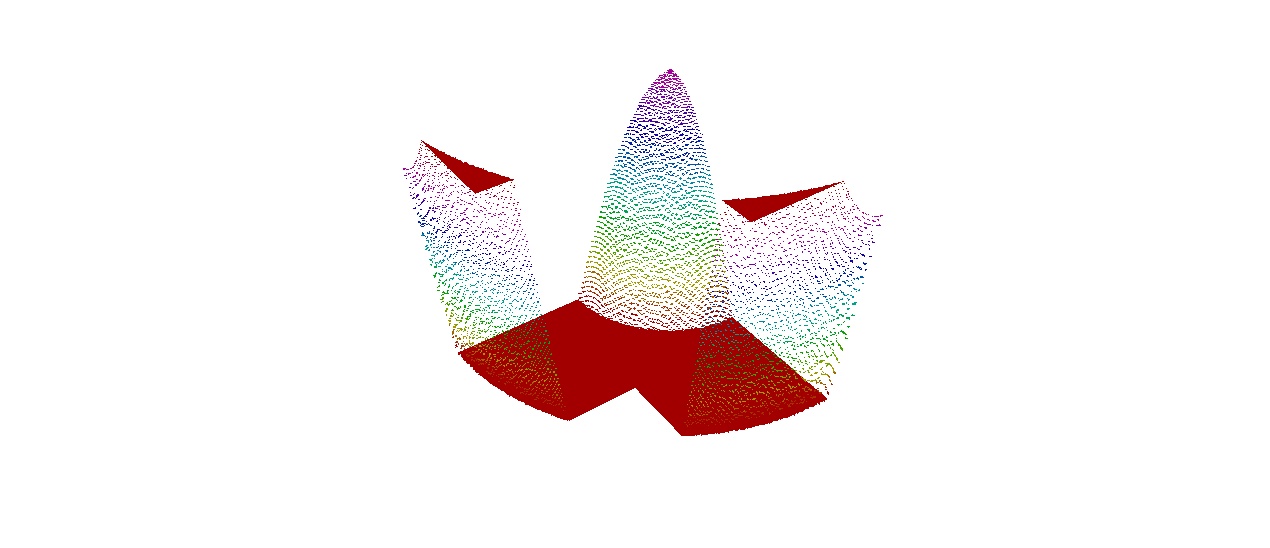The exact and discrete control profiles are depicted in Figure 1.

Next, we verify the findings from Section 5 of our studies. The error estimators derived in Section 5, are utilized as the error indicator in the adaptive loop.

\displaystyle\text{SOLVE}\rightarrow\text{ESTIMATE}\rightarrow\text{MARK}\rightarrow\text{REFINE}

The development of the space-time algorithm is based on [31]. To see the performance of a posteriori error estimators, we set the time step size $k_{n}\approx h_{K}^{2s}$ with $s=0.6$ . The space and time tolerances are taken to be $10^{-2}$ . Table 2 shows the error and convergence rate for the state, co-state and control variables in the adaptive meshes. It has been noted that the local refinement of the meshes improves the convergence rate. In Figure 2, we present the adaptive meshes at different level of refinements. Figure 2 demonstrates how effectively the mesh adapts in the vicinity of the L-shape corner and a large number of nodes is distributed along this corner.

Refer to caption — (a) Approximate control

Table 1. Errors of the state

y

, co-state

\phi

and control

u

variables on uniform meshes

Dof	N	$\\|y-Y_{h}\\|_{L^{2}(0,T;L^{2}(\Omega))}$	order	$\\|\phi-\Phi_{h}\\|_{L^{2}(0,T;L^{2}(\Omega))}$	order	$\\|u-U_{h}\\|_{L^{2}(0,T;L^{2}(\Omega))}$	order
25	4	$9.43224\times 10^{-1}$	-	$3.52156\times 10^{-1}$	-	$1.96823\times 10^{-1}$	-
81	8	$6.58948\times 10^{-1}$	0.6101	$2.37896\times 10^{-1}$	0.6672	$1.32783\times 10^{-1}$	0.6695
289	16	$4.39783\times 10^{-1}$	0.6359	$1.57783\times 10^{-1}$	0.6457	$8.75573\times 10^{-2}$	0.6549
1089	32	$2.82896\times 10^{-1}$	0.6652	$9.98987\times 10^{-2}$	0.6891	$5.64994\times 10^{-2}$	0.6604
4225	64	$1.79678\times 10^{-1}$	0.6696	$6.37896\times 10^{-2}$	0.6617	$3.62287\times 10^{-2}$	0.6555

Table 2. Errors of the state

y

, co-state

\phi

and control

u

variables on adaptive meshes

Dof	N	$\\|y-Y_{h}\\|_{L^{2}(0,T;L^{2}(\Omega))}$	order	$\\|\phi-\Phi_{h}\\|_{L^{2}(0,T;L^{2}(\Omega))}$	order	$\\|u-U_{h}\\|_{L^{2}(0,T;L^{2}(\Omega))}$	order
36	4	$8.26735\times 10^{-1}$	-	$1.39846\times 10^{-1}$	-	$9.35682\times 10^{-1}$	-
209	8	$3.29768\times 10^{-1}$	1.0451	$5.95639\times 10^{-2}$	0.9705	$4.17895\times 10^{-1}$	0.9166
417	16	$2.25869\times 10^{-1}$	1.0957	$4.19460\times 10^{-2}$	1.0153	$2.96932\times 10^{-1}$	0.9894
615	32	$1.86984\times 10^{-1}$	0.9725	$3.39783\times 10^{-2}$	1.0844	$2.43673\times 10^{-1}$	1.0175
1445	64	$1.19182\times 10^{-1}$	1.0570	$2.15249\times 10^{-2}$	1.0714	$1.56695\times 10^{-1}$	1.0363

Acknowledgements. The author wishes to thank the anonymous referees for their valuable comments and constructive suggestions that lead to the improvement of the content of the manuscript.

References

[1] R. A. Adams and J. J. F. Fournier, Sobolev Spaces, Pure and Applied Mathematics, Elsevier, Amsterdam, 2003.
[2] T. Apel, A. Rösch and G. Winkler, Optimal control in nonconvex domains: A priori discretization error estimates, Calcolo, 44(2007), pp. 137-158.
[3] I. Babuška, Finite element method for domain with corners, Computing, 6(1970), pp. 264-273.
[4] I. Babuška and W. C. Rheinboldt, Error estimates for adaptive finite element computations, SIAM J. Numer. Anal., 15(1978), pp. 736-754.
[5] C. Bacuta, J. H. Bramble and J. E. Pasciak, New interpolation results and applications to finite element methods for elliptic boundary value problems, East-West J. Numer. Math., 3(2001), pp. 179-198.
[6] C. Bacuta, J. H. Bramble and J. Xu, Regularity estimates for elliptic boundary value problems in Besov spaces, Math. Comp., 72(2003), pp. 1577-1595.
[7] R. Becker, H. Kapp and R. Rannacher, Adaptive finite element methods for optimal control of partial differential equations: Basic concept, SIAM J. Control Optim., 39(2000), pp. 113-132.
[8] L. Boccardo and T. Gallouët, Nonlinear elliptic and parabolic equations involving measure data, J. Funct. Anal., 87(1989), pp. 149-169.
[9] L. Boccardo, A. Dall’aglio and T. Gallouët, Nonlinear parabolic equations with measure data, J. Funct. Anal., 147(1997), pp. 237-258.
[10] E. Casas, Pontryagin’s principle for state constrained boundary control problems of semilinear parabolic equations, SIAM J. Control Optim., 35(1997), pp. 1297-1327.
[11] E. Casas, C. Clason and K. Kunisch, Parabolic control problems in measure spaces with sparse solutions, SIAM J. Control Optim., 51(2013), pp. 28-63.
[12] P. Chatzipantelidis, R. D. Lazarov, V. Thomée and L. B. Wahlbin, Parabolic finite element equations in nonconvex polygonal domains, BIT Numer. Math., 46(2006), pp. 113-143.
[13] P. Chatzipantelidis, R. D. Lazarov and V. Thomée, Parabolic finite volume element equations in nonconvex polygonal domains, Numer. Methods Partial Differential Equations, 2008, pp. 507-525.
[14] K. Chrysafinos and L. S. Hou, Error estimates for semidiscrete finite element approximations of linear and semilinear parabolic equations under minimal regularity assumptions, SIAM J. Numer. Anal., 40(2002), pp. 282-306.
[15] P. G. Ciarlet, The Finite Element Method for Elliptic Problems, North-Holland: Amsterdam 1978.
[16] R. Falk, Approximation of a class of optimal control problems with order of convergence estimates, J. Math. Anal. Appl., 44(1973), pp. 28-47.
[17] T. Geveci, On the approximation of the solution of an optimal control problem governed by an elliptic equation, RAIRO Anal. Numér., 13(1979), pp. 313-328.
[18] W. Gong, Error estimates for finite element approximations of parabolic equations with measure data, Math. Comp., 82(2013), pp. 69-98.
[19] W. Gong, M. Hinze and Z. Zhou, A priori error analysis for finite element approximation of parabolic optimal control problems with pointwise control, SIAM J. Control Optim., 52(2014), pp. 97-119.
[20] P. Grisvard, Elliptic Problems in Nonsmooth Domains, Pitman, MA, 1985.
[21] P. Grisvard, Singularities in Boundary Value Problems, Masson/Springer, Paris-Berlin, 1992.
[22] F. Hecht, New development in FreeFem++, J. Numer. Math., 20(2012), pp. 251-265.
[23] G. Knowles, Finite element approximation of parabolic time optimal control problems, SIAM J. Control Optim., 20(1982), pp. 414-427.
[24] K. Kufner, O. John and S. Fucik, Function Spaces, Nordhoff, Leiden, The Netherlands, 1977.
[25] R. Li, W. Liu, and N. Yan, A posteriori error estimates of recovery type for disributed convex optimal control problems, J. Sci. Comput., 33 (2007), pp. 155–182.
[26] J. L. Lions, Optimal Control of Systems Governed by Partial Differential Equations, Springer-Verlag, Berlin, 1971.
[27] J. L. Lions and E. Magenes, Nonhomogeneous Boundary Value Problems and Applications, Springer-Verlag, Berlin, 1972.
[28] W. B. Liu and N. Yan, A posteriori error estimates for distributed convex optimal control problems, Adv. Comput. Math., 15(2001), pp. 285-309.
[29] W. B. Liu and N. Yan, A posteriori error estimates for optimal control problems governed by parabolic equations, Numer. Math., 93(2003), pp. 497-521.
[30] K. Malanowski, Convergence of approximations vs. regularity of solutions for convex, control constrained optimal control problems, Appl. Math. Optim., 8(1982), pp. 69-95.
[31] R. Manohar and R. K. Sinha, A posteriori error estimates for parabolic optimal control problems with controls acting on lower dimensional manifolds, J. Sci. Comput., 89(2021), article no. 39.
[32] D. Meidner, R. Rannacher and B. Vexler, A priori error estimates for finite element discretizations of parabolic optimization problems with pointwise state constraints in time, SIAM J. Control Optim., 49(2011), pp. 1961-1997.
[33] D. Meidner and B. Vexler, A priori error estimates for space-time finite element discretization of parabolic optimal control problems Part I: Problems without control constraints, SIAM J. Control Optim., 47(2008), pp. 1150-1177.
[34] D. Meidner and B. Vexler, A priori error estimates for space-time finite element discretization of parabolic optimal control problems Part II: Problems with control constraints, SIAM J. Control Optim., 47(2008), pp. 1301-1329.
[35] D. Meidner and B. Vexler, A priori error analysis of the Petro-Galerkin Crank-Nicolson scheme for parabolic optimal control problems, SIAM J. Control Optim., 49(2011), pp. 2183-2211.
[36] P. Neittaanmaki and D. Tiba, Optimal Control of Nonlinear Parabolic Systems: Theory, Algorithms and Applications, Marcel Dekker, New York, 1994.
[37] I. Neitzel and B. Vexler, A priori error estimates for space-time finite element discretization of semilinear parabolic optimal control problems, Numer. Math., 120(2012), pp. 345-386.
[38] P. Shakya and R. K. Sinha, A posteriori error analysis for finite element approximations of parabolic optimal control problems with measure data, Appl. Numer. Math., 136(2019), pp. 23-45.
[39] P. Shakya and R. K. Sinha, Finite element approximations of parabolic optimal control problem with measure data in time, Appl. Anal., 100(2021), pp. 2706-2734.
[40] T. Sun, L. Ge, and W. Liu, Equivalent a posteriori error estimates for a constrained optimal control problem governed by parabolic equations, Inter. J. Numer. Anal. Model., 10 (2013), pp. 1–23.
[41] Y. Tang and Y. Chen, Recovery type a posteriori error estimates of fully discrete finite element methods for general convex parabolic optimal control problems, Numer. Math. Theor. Meth. Appl., 5 (2012), pp. 573–591.
[42] R. Winther, Error estimates for a Galerkin approximation of a parabolic control problems, Ann. Mat. Pura Appl., 117(1978), pp. 173-206.
[43] C. Xiong and Y. Li, A posteriori error estimates for optimal distributed control governed by the evolution equations, Appl. Numer. Math., 61 (2011), pp. 181–200.

	$\displaystyle\\|\eta\\|_{H^{1}(0,T;L^{2}(\Omega))}+\\|\eta\\|_{L^{2}(0,T;H^{1+s}(\Omega))}$	$\displaystyle\leq C_{R}\\|g\\|_{L^{2}(0,T;L^{2}(\Omega))},$
	$\displaystyle\\|\eta(\cdot,0)\\|_{H^{1}(\Omega)}$	$\displaystyle\leq C_{R}\\|g\\|_{L^{2}(0,T;L^{2}(\Omega))},$

	$\displaystyle\\|y-{Y}_{h}(u)\\|_{L^{2}(0,T;L^{2}(\Omega))}$	$\displaystyle\leq C(h^{2s}k^{-\frac{1}{2}}+k^{\frac{1}{2}}+h^{s})\Big{\{}\\|y_{0}\\|_{L^{2}(\Omega)}+\\|\sigma\\|_{L^{\infty}(0,T;L^{2}(\Omega))}\\|\tau\\|_{\mathfrak{B}[0,T]}$
(4.3)			$\displaystyle\quad\quad+\\|u\\|_{L^{2}(0,T;L^{2}(\Omega))}\Big{\}},$
	$\displaystyle\\|\phi-\Phi_{h}(u)\\|_{L^{2}(0,T;L^{2}(\Omega))}$	$\displaystyle\leq C(h^{2s}k^{-\frac{1}{2}}+k^{\frac{1}{2}}+h^{s})\Big{\{}\\|y_{h}^{n}(u)\\|_{L^{2}(0,T;L^{2}(\Omega))}+\\|P_{k}^{n}y_{d}\\|_{L^{2}(0,T;L^{2}(\Omega))}\Big{\}}$
(4.4)			$\displaystyle\quad\quad+Ck\\|y_{d,t}\\|_{L^{2}(0,T;L^{2}(\Omega))}+C\\|y-{Y}_{h}(u)\\|_{L^{2}(0,T;L^{2}(\Omega))}$

	$\displaystyle\\|\eta^{n-1}-P_{k}^{n}\mathcal{P}_{h}^{1}\eta\\|_{L^{2}(\Omega)}$	$\displaystyle\leq\\|\eta^{n-1}-P_{k}^{n}\eta\\|_{L^{2}(\Omega)}+\\|P_{k}^{n}\eta-P_{k}^{n}\mathcal{P}_{h}^{1}\eta\\|_{L^{2}(\Omega)}$
(4.8)			$\displaystyle\leq\\|\eta^{n-1}-P_{k}^{n}{\eta}\\|_{L^{2}(\Omega)}+Ch^{2s}\\|P_{k}^{n}{\eta}\\|_{H^{1+s}(\Omega)}.$

	$\displaystyle\|F_{2}\|$	$\displaystyle\leq C\Big{(}\sum_{n=1}^{N}h^{4s}\\|P_{k}^{n}\eta\\|_{H^{1+s}(\Omega)}^{2}+k_{n}\\|\eta_{t}\\|^{2}_{L^{2}(I_{n};L^{2}(\Omega))}\Big{)}^{\frac{1}{2}}$
		$\displaystyle\leq C\Big{(}\sum_{n=1}^{N}h^{4s}k_{n}^{-1}\\|P_{k}^{n}{\eta}\\|_{L^{2}(I_{n};H^{1+s}(\Omega))}^{2}+k_{n}\\|\eta_{t}\\|^{2}_{L^{2}(I_{n};L^{2}(\Omega))}\Big{)}^{\frac{1}{2}}$
		$\displaystyle\leq C(h^{2s}k^{-\frac{1}{2}}+k^{\frac{1}{2}})\\|g\\|_{L^{2}(0,T;L^{2}(\Omega))},$

	$\displaystyle\|I_{2}\|$	$\displaystyle=\Big{\|}\langle\sigma\tau,\eta\rangle_{\Omega_{T}}-\sum_{n=1}^{N}\int_{t_{n-1}}^{t_{n}}\langle\sigma\tau,P_{k}^{n}\mathcal{P}_{h}^{1}\eta\rangle_{I_{n}}\,dt\Big{\|}$
		$\displaystyle=\Big{\|}\sum_{n=1}^{N}\int_{t_{n-1}}^{t_{n}}\int_{\Omega}\sigma(x,t)(\eta-P_{k}^{n}\mathcal{P}_{h}^{1}\eta)(x)\,dxd\tau(t)\Big{\|}$
(4.12)			$\displaystyle\leq C\\|\sigma\\|_{L^{\infty}(0,T;L^{2}(\Omega))}\\|\tau\\|_{\mathfrak{B}[0,T]}\\|\eta-P_{k}^{n}\mathcal{P}_{h}^{1}\eta\\|_{L^{\infty}(0,T;L^{2}(\Omega))}.$