Erosion of synchronization and its prevention among noisy oscillators with simplicial interactions

Introduction. Synchronization is a major subject of study not only in physics but also in chemistry, biology, engineering, and sociology [1, 2, 3, 4, 5]. Examples include pacemaker cells in the heart [6], laser arrays [7], applauding audiences [8, 9], power grids consisting of AC (alternating current) generators [10], and Josephson junctions [11, 12]. In addition to synchronization, understanding the desynchronization process in oscillator assemblies is likewise very important. For example, whereas synchronization of circadian pacemaker cells in the brain is essential for mammals to have 24-hour activity rhythm, their transient desynchronization, triggered by a phase shift of light-dark cycles, is a putative cause of jet lag symptoms [13, 14]. Desynchronization is also important in neurological disorders such as Parkinson’s disease [15] and epilepsy [16], and methods to promote desynchronization in this context have been actively studied both theoretically and experimentally [17].

Phase oscillator models, including Kuramoto’s model [18], are widely known for their usefulness, not only in understanding synchronization [2, 19], but also in controlling real-world systems [20, 21]. Whereas the classical Kuramoto model considers pairwise interactions between oscillators, recent studies have extended the model to allow for non-pairwise interactions [22, 23, 24, 25]. Such structures are often called simplexes, where $n$-simplex describes an interaction between $n+1$ oscillators [26]. Research on brain dynamics [27, 28] or social phenomena [29] suggested that simplicial structures play an important role in such systems.

In noiseless phase oscillators with two-simplex interactions, Tanaka and Aoyagi [22] noted that multiple stable synchronized states appear as two clusters with different population ratios. Moreover, Skardal and Arenas showed that abrupt desynchronization transitions occur as the interaction strength decreases [23]. Skardal and Arenas also found that two- and three-simplicial couplings promote abrupt synchronization transitions in the presence of one-simplex interactions [24]. In contrast, in noisy phase oscillators, Komarov and Pikovsky pointed out that no stable synchronized states exist in the limit of an infinite number of oscillators. However, their focus was on the synchronized states that exist only in small populations. Desynchronization is expected in a large population, and as mentioned above, understanding its process is essential.

In the present study, we consider a large population of noisy phase oscillators with two-simplex coupling. Although steady synchronized states do not exist in this system, we demonstrate that the population is transiently synchronized for an extended period and then abruptly desynchronized when two-simplex coupling is sufficiently strong compared to the noise strength. Assuming weak noise and exploiting Kramers’ rate theory, we derive a closed dynamical equation for the Kuramoto order parameter by which the desynchronization process is reproduced and the exponential dependence of the lifetime of the synchronized states on the coupling strength is derived. We also consider a system in which both one- and two-simplex coupling exist and show that synchronized states become persistent when one-simplex coupling is sufficiently strong. Our bifurcation analysis reveals that the desynchronization-synchronization transition changes from continuous to discontinuous at a critical strength of two-simplex coupling.

Model and results. We consider a system of identical phase oscillators subjected to independent noise and globally coupled with one-simplex (i.e., two-body) and two-simplex (i.e., three-body) interactions, given as

$\displaystyle\dot{\theta}_{m}=\omega_{m}+$

$\displaystyle\cfrac{K_{1}}{N}\sum_{j=1}^{N}\sin(\theta_{j}-\theta_{m})+\cfrac{K_{2}}{N^{2}}\sum_{j,k=1}^{N}\sin(\theta_{j}+\theta_{k}-2\theta_{m})+\xi_{m}(t),$

(1)

where $\omega_{m}$ and $\theta_{m}$ are the intrinsic frequency and the phase of oscillator $m$ ($1\leq m\leq N$), respectively; $K_{1}\geq 0$ and $K_{2}\geq 0$ are the coupling strengths of one-simplex and two-simplex interactions, respectively. The term $\xi_{m}(t)$ represents Gaussian white noise with zero mean, $\delta$-correlated in time and independent for different oscillators. Specifically, $\langle\xi_{m}(t)\rangle=0,\ \langle\xi_{m}(t)\xi_{n}(\tau)\rangle=2D\delta_{mn}\delta(t-\tau)$, where $D\geq 0$ is the noise strength. As for the intrinsic frequencies, we consider two cases: (i) $\omega_{m}=\omega_{0}$ for all $m$, and (ii) $\omega_{m}$ is drawn from the Lorentzian distribution. Essentially, $\omega_{m}\sim g(\omega)$, where $g(\omega)=\frac{\gamma}{\pi[(\omega-\omega_{0})^{2}+\gamma^{2}]}$, $\omega_{0}$ is the mean frequency, and $\gamma$ is the width of the Lorentzian distribution. We may set arbitrary $\omega_{0}$ and $\gamma$ values without loss of generality because the model is invariant under the transformations $\theta_{m}\to\theta_{m}-\omega_{0}t$, $t\to c\gamma t$, $K_{i}\to\frac{K_{i}}{c\gamma}$, and $D\to\frac{D}{c\gamma}$, with $c$ being an arbitrary constant. Specifically, we set $\omega_{0}=0$ and $\gamma=0.01$ hereafter. Next, we introduce

$\displaystyle Z(t)=R(t)e^{i\Theta(t)}=:\cfrac{1}{N}\sum_{j=1}^{N}e^{i\theta_{j}(t)},$

(2)

where $R$ and $\Theta$ are the Kuramoto order parameter and the mean phase, respectively. Note that $R$ assumes $1$ and $0$ for the in-phase state (i.e., $\theta_{j}=\theta_{0}$ for all $j$) and the fully desynchronized state (i.e., $\theta_{j}$ is uniformly distributed within $[0,2\pi)$), respectively. Using $R$ and $\Theta$, Eq. (1) may be rewritten as

$\displaystyle\dot{\theta}_{m}=\omega_{m}$

$\displaystyle+K_{1}R\sin(\Theta-\theta_{m})+K_{2}R^{2}\sin 2(\Theta-\theta_{m})+\xi_{m}(t).$

(3)

We can see that the three-body interaction tends to make $\theta_{m}$ to be either $\Theta$ or $\Theta+\pi$. Therefore, one can suspect that three-body interaction is likely to promote the formation of two-cluster states. This is actually the case for $K_{1}=D=0$ [23]. Motivated by this observation, we numerically investigate the dynamics for the initial condition of two-cluster states. Specifically, we set $\theta_{m}(0)=0$ and $\pi$ for $1\leq m\leq\eta N$ and otherwise, respectively, where $\eta\leq\frac{1}{2}$ is the initial population ratio of the two clusters. Note that $\eta=1$ corresponds to the one-cluster state, i.e., in-phase synchrony. In Fig. 1(a), we illustrate the time evolution of the order parameter $R$ for $\omega_{m}=\omega_{0}(=0)$. For $K_{1}=0$ and $D=0.0$ (black solid line), we observe that $R$ is almost constant, indicating that the two-cluster state is stable. However, in the presence of noise, we observe qualitatively different behaviors. For $K_{1}=0$ and $D=0.1$ (purple solid line), $R$ first slowly decreases and then abruptly vanishes. Thus, the two-cluster state is, in the presence of noise, actually not stable but meta-stable with a long lifetime. Instead, the fully desynchronized state seems to be stable. The phase distributions of this process are shown in Fig. 1(c). In contrast, for $K_{1}=0.3$ and $D=0.1$ (blue solid line), $R$ seems to approach a particular nonvanishing value. For this parameter set, we also test the initial condition of the fully desynchronized state (dotted line) and observe the evolution of the phase distributions [Fig. 1(d)], noting that the system approaches a particular two-cluster state independently of the initial condition. Figure 1(b) displays results for $\omega_{m}\sim g(\omega)$, which indicates that most results are quantitatively almost unchanged, except that the lifetime of the two-cluster states for $K_{1}=0.3,D=0.1$ becomes shorter. Therefore, we expect that the essential properties of the system are shared by the cases $\omega_{m}=\omega_{0}$ and $\omega_{m}\sim g(\omega)$, and henceforth we focus on the simpler case $\omega_{m}=\omega_{0}$ for ease of analysis.

We now construct a theory to understand the synchronization and desynchronization processes. For analytical tractability, we consider a continuum limit $N\to\infty$. Specifically, the number of oscillators having the phase within $(\theta,\theta+d\theta)$ is described by $NP(\theta,t)d\theta$, where $P(\theta,t)$ is the probability density function. The order parameters are redefined as

$\displaystyle Z(t)=\int_{0}^{2\pi}\exp(i\theta)P(\theta,t)\mathrm{d}\theta.$

(4)

The Fokker–Planck equation equivalent to the Langevin equation (3) is

$\displaystyle\cfrac{\partial P}{\partial t}$

$\displaystyle=\cfrac{\partial}{\partial\theta}\left[K_{1}\sin(\theta-\Theta)+K_{2}R^{2}\sin 2(\theta-\Theta)\right]P+D\cfrac{\partial^{2}P}{\partial\theta^{2}}.$

(5)

We assume that $\Theta(t)$ is a constant in the limit $N\to\infty$. Thus, without loss of generality, we set $\Theta=0$. Note that $Z(t)=R(t)$ for $\Theta=0$. The stationary distribution $P=P_{\mathrm{s}}(\theta)$ for a constant $R=R_{s}$ can be obtained by setting $\partial_{t}P=0$, yielding

$\displaystyle P_{\mathrm{s}}(\theta)=c_{1}\exp\left(\cfrac{2K_{1}R_{s}\cos\theta+K_{2}R_{s}^{2}\cos 2\theta}{2D}\right),$

(6)

where $c_{1}$ is a normalizing constant [see SI for details]. Plugging this into Eq. (4), we obtain the self-consistency for $R_{s}$, given as

$\displaystyle R_{s}$

$\displaystyle=\int_{0}^{2\pi}P_{\rm s}(\theta)\cos\theta\ \rm{d}\theta.$

(7)

We observe that the right-hand side of Eq. (7) vanishes for $K_{1}=0$ because $P_{\mathrm{s}}(\theta)$ is $\pi$-periodic. This implies that for $K_{1}=0$, there is no stationary distribution except the one corresponding to $R_{s}=0$, which is the uniform distribution $P_{\rm s}(\theta)=\frac{1}{2\pi}$ [30]. Nontrivial steady distributions may only arise when $K_{1}>0$.

We investigate the bifurcation of the system by numerically solving Eq. (7) for $R_{\rm s}$. In Fig. 2(a), we plot some typical behavior of Eq. (7), indicating that the steady state of $R_{s}$ bifurcates as $K_{1}$ and $K_{2}$ vary. In Fig. 2(b), the phase diagram in the $(K_{1},K_{2})$ plane is displayed, suggesting that the bifurcation occurs at $K_{1}=K_{\rm c}=0.2$ for all $K_{2}$. In Figs. 2(c) and (d), we plot $R_{s}$ as a function of $K_{1}$ for $K_{2}=0.15$ and $K_{2}=3.0$, respectively. We find that supercritical and subcritical pitchfork bifurcations occur in Figs. 2(c) and (d), respectively. Moreover, the bifurcation type changes from supercritical to subcritical at $K_{1}\simeq 0.2$, yielding the bistable region in which both the desynchronized and synchronized states are stable for $K_{1}>0.2$. Note that $0.2$ is equal to $2D$.

To elucidate the bifurcation structure, we perform a weakly nonlinear analysis using a standard method [18, 3]. We denote the bifurcation point of $R=0$ by $K_{1}=K_{\rm c}$ and set $K_{1}=K_{\rm c}(1+\mu)$, where $\mu$ is the bifurcation parameter. The complex order parameter is expanded as

$\displaystyle Z=\varepsilon Z_{1}+\varepsilon^{2}Z_{2}+\cdots,$

(8)

where $\epsilon=\sqrt{|\mu|}$. As detailed in SI, we derive

$\displaystyle\cfrac{1}{\varepsilon^{2}}\dot{Z}_{1}=\cfrac{K_{1}-K_{\rm c}}{2}\ Z_{1}-g|Z_{1}|^{2}Z_{1},$

(9)

where

	$\displaystyle K_{\rm c}$	$\displaystyle=2D,$		(10)
	$\displaystyle g$	$\displaystyle=\cfrac{K_{\rm c}^{2}+K_{\rm c}K_{2}}{8D}-\cfrac{K_{2}}{2}.$		(11)

Note that $g$ is real in this particular system. The sign of $g$ determines the bifurcation type: supercritical and subcritical bifurcations occur for $g>0$ (or $K_{2}<K_{\rm c}$) and $g<0$ (or $K_{2}>K_{\rm c}$), respectively. This theoretical analysis is in perfect agreement with the numerical analysis of Eq. (7) shown in Fig. 2.

Next, we investigate the slow desynchronization process that occurs for $K_{1}=0$ (see Fig.1(c)). We will demonstrate that under some assumptions, an approximate dynamical equation for $R$ may be obtained in a closed form, by which we may determine the lifetime of the synchronized state. To this end, we first rewrite the system as a gradient system:

$\displaystyle\dot{\theta}_{m}$

$\displaystyle=-\cfrac{\partial}{\partial\theta}\ U(\theta,R(t))+\xi_{m},$

(12)

where

$\displaystyle U(\theta,R)$

$\displaystyle=-\cfrac{1}{2}\ K_{2}R^{2}\cos 2\theta$

(13)

is the potential. Clearly, there are minima at $\theta=0$ and $\pi$ in this potential $R>0$, which have the same depth and are separated by the potential barrier $\Delta U$ given by

$\displaystyle\Delta U=K_{2}R^{2}.$

(15)

We assume that the noise is sufficiently weak compared to $\Delta U$, i.e., $D\ll\Delta U$. We also assume that $R$ evolves sufficiently slowly. Then, we can expect that the phase distribution is well approximated to

$\displaystyle P(\theta,t)=\eta(t)\delta(\theta)+(1-\eta(t))\delta(\theta-\pi).$

(16)

Under our assumption, each oscillator experiences the virtually fixed potential and jumps from one well to another at a certain rate $k$, i.e.,

$\displaystyle\dot{\eta}=-k\eta+k(1-\eta)=k(1-2\eta).$

(17)

According to Kramers’ rate theory [31, 32], we may calculate $k$ based on $U$ as follows:

	$\displaystyle k(R)$	$\displaystyle=2\cfrac{\sqrt{|\partial_{\theta}^{2}U(\theta_{\min},R)\partial_{\theta}^{2}U(\theta_{\max},R)}|}{2\pi}\exp\left(-\cfrac{\Delta U}{D}\right)$		(18)
		$\displaystyle=\cfrac{2K_{2}R^{2}}{\pi}\exp\left(-\cfrac{K_{2}R^{2}}{D}\right),$		(19)

where the rate is doubled compared to the standard formula [32] because there are two paths for oscillators to move from one well to another. We assume $\eta\geq\frac{1}{2}$ without loss of generality. Then, under the assumption of (16), we obtain $R=2\eta-1$. Substituting (17) into $\dot{R}=2\dot{\eta}$, we obtain the closed equation for $R(t)$ as

$\displaystyle\dot{R}(t)=-\cfrac{4K_{2}R^{3}}{\pi}\exp\left(-\cfrac{K_{2}R^{2}}{D}\right).$

(20)

Because $\dot{R}<0$ for $R>0$ and $\dot{R}=0$ for $R=0$, $R=0$ is the global attractor. However, because the term $\exp\left(-\cfrac{K_{2}R^{2}}{D}\right)$ is vanishingly small for $R\gg\sqrt{\frac{D}{K_{2}}}\equiv R_{1}$, the relaxation to $R=0$ is extremely slow if $R(0)\equiv R_{0}\gg R_{1}$. We define the lifetime $\tau$ of the synchronized state as the time within which $R$ varies from $R_{0}$ to $R_{1}$. Because $\tau=\int_{0}^{\tau}dt=\int_{R_{0}}^{R_{1}}\frac{dt}{dR}dR$, we obtain

$\displaystyle\tau$

$\displaystyle=\int_{R_{1}}^{R_{0}}\cfrac{\pi\exp\left(\frac{K_{2}R^{2}}{D}\right)}{4K_{2}R^{3}}\ \mathrm{d}R.$

(21)

This integral can only be computed numerically. Because the evolution of $R(t)$ is very slow until $R$ reaches $R_{1}$, a rough estimation of $\tau$ may be given by setting $R(t)=R_{0}$ in Eq. (21), giving rise to

$\displaystyle\tau\sim e^{\frac{K_{2}R_{0}^{2}}{D}},$

(22)

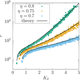
where the coefficient including the factor $\frac{R_{0}-R_{1}}{R_{1}^{3}}$ is omitted. This estimation indicates that $\tau$ approximately exponentially increases with $K_{2}$. To verify our theory, in Fig. 3, we compare our theoretical estimations, given by Eqs. (21) and (22), to the lifetime obtained from direct simulations of Eq. (1). The simulation setup is the same as that illustrated in Fig. 1, and the lifetime is given as the time at which $R$ passes $R_{1}$ for the first time. We observe that Eq. (21) is in reasonable agreement with the simulation data. We also observe that the lifetime indeed increases approximately exponentially with $K_{2}$, as predicted by Eq. (22). Note that as detailed in SI, the closed equation for $R$ may also be obtained for $K_{1}>0$ and it approximately reproduces $R(t)$ trajectories obtained in Eq. (1).

Conclusion. In this study, we explored a large population of noisy oscillators with one- and two-simplicial interactions. Specifically, we demonstrated that dynamical noise, no matter how weak, will extinguish steady synchronized states when only two-simplicial interaction exists. However, synchronized states composed of two clusters persist for extended periods. This feature could translate to future applications. In the context of memory storage, a cluster can be considered as a state in which the system holds some information. Since the lifetime of a cluster state is determined by the initial ratio of clusters, it may be possible to design a self-organizing system that can measure time and also pre-set the time to retain information.

Finally, we discuss the limitations and future directions of this study. We have considered only the all-to-all coupling case. Although such a network is mathematically tractable, its applicability to real-world systems would be limited. Extension to complex networks is vital. Furthermore, to comprehensively understand the nature of two-simplex interaction, it is essential to explore another generic coupling type, given as $\sin(\theta_{j}-\theta_{k}-\theta_{m})$ instead of $\sin(2\theta_{j}+\theta_{k}-2\theta_{m})$ in Eq. (1) [33, 24]. The noise effect on such a system is an interesting open problem.

References

- Winfree [2001] A. T. Winfree, The geometry of biological time (Springer-Verlag New York, 2001).
- Kuramoto [1984] Y. Kuramoto, Chemical Oscillations, Waves, and Turbulence (Springer-Verlag Berlin Heidelberg, 1984).
- Pikovsky et al. [2001a] A. Pikovsky, J. Kurths, M. Rosenblum, and J. Kurths, Synchronization: A Universal Concept in Nonlinear Sciences (Cambridge University Press, 2001).
- Glass [2001] L. Glass, Synchronization and rhythmic processes in physiology, Nature 410, 277 (2001).
- Eilam [2019] E. Eilam, Synchronization: a framework for examining emotional climate in classes, Palgrave Communications 5, 1 (2019).
- Glass and Mackey [2020] L. Glass and M. C. Mackey, From Clocks to Chaos: The Rhythms of Life (Princeton University Press, 2020).
- Simonet et al. [1994] J. Simonet, M. Warden, and E. Brun, Locking and arnold tongues in an infinite-dimensional system: The nuclear magnetic resonance laser with delayed feedback, Phys. Rev. E Stat. Phys. Plasmas Fluids Relat. Interdiscip. Topics 50, 3383 (1994).
- Néda et al. [2000] Z. Néda, E. Ravasz, T. Vicsek, Y. Brechet, and A. L. Barabási, Physics of the rhythmic applause, Phys. Rev. E Stat. Phys. Plasmas Fluids Relat. Interdiscip. Topics 61, 6987 (2000).
- Neda et al. [2000] Z. Neda, E. Ravasz, Y. Brechet, T. Vicsek, and A.-L. Barabási, The sound of many hands clapping: Tumultuous applause can transform itself into waves of synchronized clapping, Nature 403, 849 (2000).
- Rohden et al. [2012] M. Rohden, A. Sorge, M. Timme, and D. Witthaut, Self-organized synchronization in decentralized power grids, Phys. Rev. Lett. 109, 064101 (2012).
- Wiesenfeld et al. [1996] K. Wiesenfeld, P. Colet, and S. H. Strogatz, Synchronization transitions in a disordered josephson series array, Phys. Rev. Lett. 76, 404 (1996).
- Wiesenfeld et al. [1998] K. Wiesenfeld, P. Colet, and S. H. Strogatz, Frequency locking in josephson arrays: Connection with the kuramoto model, Phys. Rev. E 57, 1563 (1998).
- Yamaguchi et al. [2013] Y. Yamaguchi, T. Suzuki, Y. Mizoro, H. Kori, K. Okada, Y. Chen, J.-M. Fustin, F. Yamazaki, N. Mizuguchi, J. Zhang, et al., Mice genetically deficient in vasopressin v1a and v1b receptors are resistant to jet lag, Science 342, 85 (2013).
- Kori et al. [2017] H. Kori, Y. Yamaguchi, and H. Okamura, Accelerating recovery from jet lag: prediction from a multi-oscillator model and its experimental confirmation in model animals, Scientific reports 7, 46702 (2017).
- Popovych and Tass [2018] O. V. Popovych and P. A. Tass, Multisite delayed feedback for electrical brain stimulation, Frontiers in Physiology 9, 46 (2018).
- Jiruska et al. [2013] P. Jiruska, M. De Curtis, J. G. Jefferys, C. A. Schevon, S. J. Schiff, and K. Schindler, Synchronization and desynchronization in epilepsy: controversies and hypotheses, The Journal of physiology 591, 787 (2013).
- Pikovsky and Rosenblum [2015] A. Pikovsky and M. Rosenblum, Dynamics of globally coupled oscillators: Progress and perspectives, Chaos: An Interdisciplinary Journal of Nonlinear Science 25 (2015).
- Kuramoto [1975] Y. Kuramoto, Self-entrainment of a population of coupled non-linear oscillators, in International Symposium on Mathematical Problems in Theoretical Physics (Springer Berlin Heidelberg, 1975) pp. 420–422.
- Pikovsky et al. [2001b] A. Pikovsky, M. Rosenblum, and J. Kurths, Synchronization: a universal concept in nonlinear sciences (Cambridge University Press, 2001).
- Kiss et al. [2007] I. Z. Kiss, C. G. Rusin, H. Kori, and J. L. Hudson, Engineering complex dynamical structures: Sequential patterns and desynchronization, Science 316, 1886 (2007).
- Kori et al. [2008] H. Kori, C. G. Rusin, I. Z. Kiss, and J. L. Hudson, Synchronization engineering: Theoretical framework and application to dynamical clustering, Chaos 18, 026111 (2008).
- Tanaka and Aoyagi [2011] T. Tanaka and T. Aoyagi, Multistable attractors in a network of phase oscillators with three-body interactions, Phys. Rev. Lett. 106, 224101 (2011).
- Skardal and Arenas [2019] P. S. Skardal and A. Arenas, Abrupt desynchronization and extensive multistability in globally coupled oscillator simplexes, Phys. Rev. Lett. 122, 248301 (2019).
- Skardal and Arenas [2020] P. S. Skardal and A. Arenas, Higher order interactions in complex networks of phase oscillators promote abrupt synchronization switching, Communications Physics 3, 1 (2020).
- Xu et al. [2020] C. Xu, X. Wang, and P. S. Skardal, Bifurcation analysis and structural stability of simplicial oscillator populations, Phys. Rev. Research 2, 023281 (2020).
- Salnikov et al. [2018] V. Salnikov, D. Cassese, and R. Lambiotte, Simplicial complexes and complex systems, Eur. J. Phys. 40, 014001 (2018).
- Giusti et al. [2016] C. Giusti, R. Ghrist, and D. S. Bassett, Two’s company, three (or more) is a simplex (2016).
- Sizemore et al. [2018] A. E. Sizemore, C. Giusti, A. Kahn, J. M. Vettel, R. F. Betzel, and D. S. Bassett, Cliques and cavities in the human connectome, J. Comput. Neurosci. 44, 115 (2018).
- Wang et al. [2020] D. Wang, Y. Zhao, H. Leng, and M. Small, A social communication model based on simplicial complexes, Phys. Lett. A 384, 126895 (2020).
- Komarov and Pikovsky [2015] M. Komarov and A. Pikovsky, Finite-size-induced transitions to synchrony in oscillator ensembles with nonlinear global coupling, Phys. Rev. E Stat. Nonlin. Soft Matter Phys. 92, 020901 (2015).
- Gardiner [2010] C. Gardiner, Stochastic Methods: A Handbook for the Natural and Social Sciences (Springer Berlin Heidelberg, 2010).
- Risken [1996] H. Risken, Fokker-Planck equation, in The Fokker-Planck Equation: Methods of Solution and Applications, edited by H. Risken (Springer Berlin Heidelberg, Berlin, Heidelberg, 1996) pp. 63–95.
- Ashwin and Rodrigues [2016] P. Ashwin and A. Rodrigues, Hopf normal form with sn symmetry and reduction to systems of nonlinearly coupled phase oscillators, Physica D: Nonlinear Phenomena 325, 14 (2016).