Ergosphere and shadow of a rotating regular black hole
Abstract
The spacetime singularities in classical general relativity predicted by the celebrated singularity theorems are formed at the end of gravitational collapse. Quantum gravity is the expected theory to resolve the singularity problem, but we are now far from it. Therefore attention has shifted to models of regular black holes free from the singularities. A spherically symmetric regular toy model was obtained by Dymnikova (1992) which we demonstrate as an exact solution of Einstein’s field equations coupled to nonlinear electrodynamics for a Lagrangian with parameter related to magnetic charge. We construct rotating counterpart of this solution which encompasses the Kerr black hole as a special case when charge is switched off (). Event Horizon Telescope has released the first image of supermassive black hole M87∗, revealing the structure near black hole horizon. The rotating regular black hole’s shadow may be useful to determine strong field regime. We investigate ergosphere and black hole shadow of rotating regular black hole to infer that their sizes are sensitive to charge and have a richer chaotic structure. In particular, rotating regular black hole possess larger size, but less distorted shadows when compared with Kerr black holes. We find one to one correspondence between ergosphere and shadow of the black hole.
I Introduction
The elegant theorems of Hawking and Penrose imply that spacetime singularities are pervasive features of general relativity, so that the theory itself predicts its own failure to describe the physics of these extreme situations. The spacetime singularities that arise in gravitational collapse are always hidden inside black holes, which is the essence of the weak cosmic censorship conjecture, put forward 40 years ago by Penrose Penrose:1969pc . This signature is still one of the most important open questions in general relativity. We are far away from any robust and reliable quantum theory of gravity capable of resolving the singularities in the interior of black holes. Hence, there is significant attention towards models of black hole solutions without the central singularity. The earliest idea of regular models dates back to the pioneering work of Sakharov Sakharov:1966 and Gliner Gliner:1966 where they proposed that the spacetime in the highly dense central region of a black hole should be de Sitter-like at . Thus spacetime filled with vacuum could provide a proper discrimination at the final stage of gravitational collapse, replacing future singularity Gliner:1966 . The prototype of these regular black holes is the Bardeen metric Bardeen:1968 , which can be formally obtained by coupling Einstein’s gravity to a nonlinear electrodynamic field AyonBeato:2000zs , thought to be an alteration of the Reissner-Nordström solution. There has been enormous attentions to obtain regular black holes Dymnikova:2004zc ; Bronnikov:2000vy ; Shankaranarayanan:2003qm ; Hayward:2005gi ; Ansoldi:2008jw ; Culetu:2014lca ; Balart:2014jia ; Balart:2014cga ; Xiang:2013sza ; most of these regular black holes were driven by the Bardeen idea Bardeen:1968 . However, these are only nonrotating black holes, which can be hardly tested by observations, as black hole spin is an important parameter in astrophysical processes.
Further, a study of rotating regular solutions is important as the astronomical observations predict that the astrophysical black hole might be a Kerr black hole Bambi:2011mj . However, the real nature of these astrophysical black holes is still to be verified Bambi:2011mj . Analyzing the iron lines and the continuum fitting method are possible procedures, which can probe the geometry of spacetime around astrophysical black holes candidates Bambi:2014nta . The rotating solutions of the Bardeen metrics have been obtained in Ref. Bambi:2011mj . There exists a number of rotating regular black holes Bambi:2013ufa ; Neves:2014aba ; Toshmatov:2014nya ; Ghosh:2014hea ; Toshmatov:2017zpr which were discovered with the help of the Newman-Janis algorithm Newman:1965tw , and also by using other techniques Azreg-Ainou:2014aqa ; Azreg-Ainou:2014nra ; Azreg-Ainou:2014pra ; Ghosh:2014pba . The authors in Refs. Ghosh:2014mea ; Amir:2015pja ; Ghosh:2015pra ; Amir:2016nti ; Ahmed:2018fge demonstrated that the regular black holes can be considered as the particle accelerator. The quasinormal modes of test fields around the regular black holes has been discussed explicitly in Toshmatov:2015wga . An interesting study on electromagnetic perturbation of the regular black holes has been discussed thoroughly in Toshmatov:2018tyo ; Toshmatov:2018ell ; Toshmatov:2019gxg .
The black hole shadow is a dark zone in the sky and the shadow is a useful tool for measuring black hole parameters because its shape and size carry impression of the geometry surrounding the black hole. Observing the black hole shadow is a possible method to determine the spin of the black hole, and this subject is popular nowadays. This triggered theoretical investigation of the black holes for wide variety of spacetimes Chandrasekhar92 ; Falcke:1999pj ; Takahashi04 ; Takahashi:2005hy ; Bambi:2008jg ; Hioki:2009na ; Bambi:2010hf ; Amarilla:2010zq ; Amarilla:2011fxx ; Abdujabbarov:2012bnn ; Yumoto:2012kz ; Li:2013jra ; Amarilla:2013sj ; Atamurotov:2013dpa ; Atamurotov:2013sca ; Wei:2013kza ; Grenzebach:2014fha ; Papnoi:2014 ; Abdujabbarov:2015xqa ; Johannsen:2015qca ; Goddi:2016jrs ; Abdujabbarov:2016hnw ; Younsi:2016azx ; Amir:2016cen ; Grenzebach:2016 ; Zakharov ; Singh:2017vfr ; Amir:2017slq ; Kumar:2017vuh . Apart from black holes, the theoretical investigation of shadow of wormholes has also been discussed in Nedkova:2013msa ; Bambi:2013nla ; AzregAinou:2014dwa ; Ohgami:2015nra ; Ohgami:2016iqm ; Abdujabbarov:2016efm ; Shaikh:2018kfv ; Amir:2018szm ; Amir:2018pcu . Hioki and Maeda Hioki:2009na discuss a simple relation between the shape of shadow, inclination angle and spin parameter for the Kerr black hole. A coordinate-independent method was proposed to distinguish the shape of black hole shadow from other rotating black holes Abdujabbarov:2015xqa . From the observational point of view, the study of shadow is significant because of the Event Horizon Telescope111https://eventhorizontelescope.org. It was setup with an aim to image the event horizon of supermassive black holes Sgr A∗ and M87∗. They have successfully released the first image of M87∗ which is in accordance with the Kerr black hole predicted by general relativity Akiyama:2019cqa ; Akiyama:2019fyp ; Akiyama:2019eap . The photon ring and shadow have been observed which open a new window to test general relativity and modified theories of gravity in strong field regime.
The purpose of this paper is to construct the rotating counterpart or Kerr-like regular black hole from the spherically symmetric regular black hole proposed by Dymnikova Dymnikova:1992ux . The black hole is singularity free or regular black hole with an additional parameter , and for definiteness, we can call it the rotating regular black hole. We investigate several properties including the shadow of this black hole to explicitly bring out the effect of parameter , and compare with the Kerr black hole. It turns out that the parameter leaves a significant imprint on the black hole shadow, and also affects the other properties.
The paper is organized as follows. In Sec. II, we show that the spherically symmetric regular black hole obtained by Dymnikova Dymnikova:1992ux is an exact solution of general relativity coupled to nonlinear electrodynamics. We introduce a line element of the rotating regular black hole spacetime and discuss associated sources with it in Sec. III. The weak energy conditions is the subject of Sec. IV. In Sec. V, we discuss some basic properties of the rotating regular black hole. Shadow of rotating regular black hole is the subject of Sec. VI where we derive analytical formulae for the shadow and we conclude in the Sec. VII. We consider the signature convention () for the spacetime metric and use the geometric unit throughout the paper.
II Nonlinear electrodynamics and exact regular black hole solution
The spherically symmetric metric proposed by Dymnikova Dymnikova:1992ux represents a regular black hole with de Sitter core instead of a singularity. The stress-energy tensor responsible for the geometry describes a smooth transition from the standard vacuum state at infinity to isotropic vacuum state through anisotropic vacuum state in the intermediate region. The spacetime metric of the Dymnikova solution reads
| (1) |
where , is the black hole mass, and the parameter is given by . The corresponding energy-momentum tensor of metric (1) is Dymnikova:1992ux
| (2) |
The metric (1) admits two horizons, i.e., the event horizon and the Cauchy horizon, but there is no singularity. We know that the horizons are zeros of , which are given Dymnikova:1992ux by
The metric (1) is regular, everywhere including at , which is evident from the behavior of the curvature invariants. Thus the metric (1) that for large coincides with the Schwarzschild solution, for small behaves like the de Sitter spacetime and describes a spherically symmetric regular black hole. In what follows, we show the metric (1) as an exact solution of general relativity coupled to an appropriate nonlinear electrodynamics.
We start with action of general relativity coupled to the nonlinear electrodynamics which is given by
| (3) |
where is the Ricci scalar and is an arbitrary function of with , and denotes the electromagnetic potential. The Einstein field equations are derived from the action (3) which read simply
| (5) | |||||
We further consider the spherically symmetric line element of the following form
| (6) |
For the spherically symmetric spacetime the only nonzero components of appropriate to magnetic charge are and with such that Fernando:2016ksb . Now it is straight forward to compute
| (7) |
where is the absolute value of magnetic field. The regular solution Dymnikova:1992ux in which we are much interested comes from particular nonlinear electrodynamics source
| (8) |
where the parameter is given by with and are arbitrary constant can be related to the magnetic charge and the black hole mass, respectively. The component of the Einstein’s field equations (5) gives
| (9) |
On substituting (8) into (9) and then integrating it results in
| (10) |
where the integration constant is purposely chosen as , thus the above equation yields
| (11) |
When we substitute (11) in (6) eventually we get the spherically symmetric Dymnikova regular spacetime (1). Thus, we can say that the Dymnikova spacetime (1) can be obtained exactly with source from a particular nonlinear electrodynamics where the source is given by the Lagrangian (8).
III Rotating regular black holes
In this section, we aim to study the rotating counterpart of the Dymnikova spacetime which is a generalization of the Kerr black hole. We start by constructing a rotating counterpart of the regular spacetime (1) which in the Boyer-Lindquist coordinates reads
| (12) | |||||
where
Here represents the rotation parameter and is the mass function given in (11). Henceforth, we use the term rotating regular black hole for the spacetime metric (12). It is noticeable that in the absence of charge (), we obtain the Kerr spacetime. The spacetime (12) has independence on and coordinates that means and coordinates are cyclic coordinates in the Lagrangian which corresponding to two Killing vectors, namely, the time translation Killing vector , and the azimuthal Killing vector .
Now we are going to check the validity of the rotating solution by computing the source nonlinear electrodynamics equations. The action and corresponding field equations are explicitly expressed in the previous section. The vector potential in case of spherically symmetric spacetime is given by . The vector potential for the rotating spacetime gets modify Toshmatov:2017zpr and given as follows
| (13) |
It is easy to compute the field strength for the rotating spacetime, which turns out to be in following form
| (14) |
We can immediately recover while substitute in (14). In order to compute the source for the rotating spacetime, we solve the Einstein field equations, with respect to and . Consequently, the Lagrangian density reads simply
| (15) |
and has the form
| (16) |
Interestingly, when we substitute into Eqs. (15) and (16) as a result we obtain
| (17) |
These expressions are exactly similar to that of the spherically symmetric spacetime.
IV Energy conditions
Now we are much interested in computing the orthonormal basis also known as tetrads of the spacetime (12) so that we can analyze the matter associated with the rotating regular spacetime Neves:2014aba ; Bardeen:1972fi . The computation of the orthonormal basis gives the following form Neves:2014aba ; Bardeen:1972fi :
| (18) |
where is the angular velocity of the rotating regular black hole. We further determine the components of the energy-momentum tensor by using the following relation Neves:2014aba ; Bardeen:1972fi
When we compute the components of the energy-momentum tensor , then we realize that it has only diagonal components Neves:2014aba ; Bardeen:1972fi , i.e.,
| (19) |
where and are the matter density and the pressure, respectively. In case of the rotating regular black hole, the quantities and that appearing in (19) have the forms as follows
| (20) |
When we compare them with the components of static counterpart (2), we find that the components of (IV) are different because of the black hole rotation. This also happens when we consider rotating Vaidya solution Carmeli:1975kg , it has in addition null radiation some another source. Having the expressions of matter density and pressure , we can verify the weak energy condition for the spacetime (12) that requires the inequalities and , () to be satisfied.
|
 
|
 
|
|
Moreover, a straight forward calculation gives
| (21) |
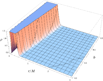
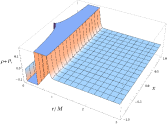
which shows that the energy condition may be violated and it can be seen in the plots (cf. Fig. 1 and 2). We find that the matter density is always positive for all values of and as can be seen from the Fig. 1. It turns out that the rotating regular black hole solution may violate energy conditions; however, this happens for all the rotating regular black holes in the literature (see, e.g., Neves:2014aba ; Bambi:2013ufa ). Despite small violation of such solutions are important from phenomenologically and also they are important as astrophysical black holes are rotating.
V Properties of rotating regular spacetime
In this section, we will discuss some important properties of the rotating regular black hole solution, for instance, the curvature scalars, the horizons, and the ergospheres etc. It is important to study these basic properties of the spacetime from physical point of view.
V.1 Curvature invariants
In order to check the curvature singularity within the spacetime, we compute the curvature invariants or scalars of the rotating regular black hole spacetime. We find that the curvature invariants of the spacetime (12) have cumbersome forms, but in the limit , they reduce to the following expressions
| (22) |
We further consider the limit of (22), in this limit they turn out to be
| (23) |
 
|
The curvature invariants have finite values for , therefore, we can say that the metric (12) is regular everywhere as can be seen from the Fig. 3. The figure shows that the Kretschmann scalar and the square of Ricci tensor are well behaving for different values of the parameters and . It is noticeable that the presence of the exponential factor in the mass of the black hole (12), i.e., , makes the black hole singularity free.
V.2 Horizons
Now we wish to discuss the effect of charge on the structure of horizons and ergosphere. It turns out that as like the Kerr black hole, the spacetime has two surfaces, viz., static limit surfaces and horizons. The static limit surface is a surface on which the time translation Killing vectors () becomes null or . It requires that the component to be vanished,
| (24) |
The typical behavior of the static limit surface is depicted in Fig. 4 for various values of the parameters (see also Table 1). It turns out that the behavior is similar to that of the Kerr black holes. However, the radii of the static limit surface shrink with increasing values of charge (Table 1).


| 0 | 1.91652 | 1.95917 | 0.04265 | 1.89303 | 1.94802 | 0.05499 | 1.86603 | 1.93541 | 0.06938 | 1.83516 | 1.92128 | 0.08612 |
|---|---|---|---|---|---|---|---|---|---|---|---|---|
| 0.20 | 1.91652 | 1.95917 | 0.04265 | 1.89303 | 1.94802 | 0.05499 | 1.86603 | 1.93541 | 0.06938 | 1.83516 | 1.92128 | 0.08612 |
| 0.40 | 1.91652 | 1.95917 | 0.04265 | 1.89303 | 1.94802 | 0.05499 | 1.86603 | 1.93541 | 0.06938 | 1.83516 | 1.92128 | 0.08612 |
| 0.80 | 1.91648 | 1.95915 | 0.04267 | 1.89298 | 1.94800 | 0.05502 | 1.86594 | 1.93539 | 0.06945 | 1.83502 | 1.92124 | 0.08622 |
| 1.10 | 1.90991 | 1.95491 | 0.04500 | 1.88464 | 1.94325 | 0.05861 | 1.85500 | 1.92997 | 0.07497 | 1.82009 | 1.91499 | 0.0949 |
| 1.20 | 1.89844 | 1.94703 | 0.04859 | 1.87049 | 1.93456 | 0.06407 | 1.83687 | 1.92027 | 0.08340 | 1.79566 | 1.90399 | 0.10833 |
| 1.30 | 1.81955 | 1.89605 | 0.07650 | 1.76301 | 1.87791 | 0.11490 | 1.79581 | 1.89955 | 0.10374 | 1.73422 | 1.88046 | 0.14624 |
Since the spacetime (12) has a coordinate singularity at , which corresponds to the horizon of the rotating regular black holes. Actually the event horizon is located at the larger root () of
| (25) |
where (24) coincides with (25) when either or . Clearly, the radii of horizons depend on the parameter and they are different from the Kerr black hole. We solve (25) for horizons numerically as well as plot them in Fig. 5 for different values of parameters and . It turns out that the horizons of the rotating regular black hole have similar behavior like the Kerr black hole, but there exist several extremal black holes corresponding to the various values of charge .


| 0 | 0.28085 | 1.91652 | 0.29917 | 1.89303 | 0.31791 | 1.86603 | 0.33734 | 1.83516 |
|---|---|---|---|---|---|---|---|---|
| 0.40 | 0.43462 | 1.91652 | 0.45736 | 1.89303 | 0.48063 | 1.86603 | 0.50460 | 1.83516 |
| 0.80 | 0.74894 | 1.91648 | 0.77631 | 1.89298 | 0.80536 | 1.86594 | 0.83625 | 1.83502 |
| 1.10 | 1.02687 | 1.90991 | 1.05876 | 1.88464 | 1.09424 | 1.85500 | 1.13402 | 1.82009 |
| 1.20 | 1.13547 | 1.89844 | 1.17071 | 1.87049 | 1.21110 | 1.83687 | 1.25840 | 1.79566 |
| 1.30 | 1.41374 | 1.81955 | 1.47841 | 1.76301 | 1.35248 | 1.79581 | 1.42108 | 1.73422 |
The Fig. 5 and Table 2 shows the existence of two roots, for a set of values of parameters and , which corresponds to the Cauchy horizon (smaller root) and event horizon (larger root). We find that for a given value of , there exists a critical value of parameter , where the two horizons coincide () corresponding to the extremal black holes (Fig. 5 and 6). When , we have rotating black hole with two horizons, and for no black hole will form (Fig. 5 and 6).
V.3 Ergosphere


|


|


|


|
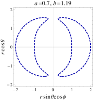
An ergosphere is bounded by the two above discussed surfaces, namely, the static limit surface and the event horizon. It lies outside the black hole. The ergoregion of the rotating black holes is a region of spacetime where the time translation Killing vector becomes spacelike, and also that every timelike vector acquires rotational () counterpart. Hence, a particle can enter into ergoregion and can leave again, but it cannot remain stationary without the ergosphere. The ergospheres for the rotating regular black hole are shown in the Fig. 6 for different values of parameters , which are polar plots of (24) and (25).
Interestingly, we note that ergosphere becomes more prolate with increasing values of charge (see Fig. 6 horizontally) and with increasing spin (see Fig. 6 from top to bottom). It means the faster rotating and charged black holes are more prolate thereby increasing the area of the ergosphere. Furthermore, we observe from the Fig. 6 that we can find a critical parameter where two surface shrinks to one, and for , we have no ergoregion. It turns out that energy can be extracted from ergoregion via Penrose process Penrose:1971uk and the magnetic charge shall affect the Penrose process.
VI Black hole shadow
In this section, we are going to study one of the most interesting astrophysical phenomena for the rotating regular black hole known as black hole shadow. This can be understood as follows. When a black hole is placed in between an observer and the bright background source, the photons with a small angular momentum fall into the black hole without reaching the observer create a dark spot in the sky, which is called the black hole shadow. Thus, to obtain the apparent shape or shadow of the black hole and discuss the properties of shadow, we must discuss the geodesic of the photon in the background of the rotating regular black hole. These geodesics can be determined by the Hamilton-Jacobi formulation Carter:1968rr given by
| (26) |
which has a solution in the separable form as follows
| (27) |
where corresponds to the rest mass of the particle, and and are respectively functions of and only. Note that in case of photon the rest mass, . By following the standard procedure of the Hamilton-Jacobi method, we obtain the following forms of the geodesic equations,
| (28) |
| (29) |
| (30) |
| (31) |
where and can be expressed as follows
| (32) |
These geodesic equations represent first-order differential equations with respect to the affine parameter and contain three constants of the motion: the energy , the angular momentum , and the Carter constant Carter:1968rr . If we substitute , in the geodesic equations, they reduce to the Kerr spacetime case Hioki:2009na . Now in order to get the shadow of the rotating regular black hole, we introduce the two independent dimensionless quantities or impact parameters such that and . Equation explores the radial turning points of the photons and the spherical photon orbits around the black hole can be determined by the following relations Bardeen:1972fi
| (33) |
On solving (33) for impact parameters and , we immediately get their forms as follows
| (34) |
It turns out that the impact parameters have a dependency on charge . If charge is set to be zero, then Eq. (34) reduces to the Kerr black hole case Hioki:2009na . This calculation is helpful to determine the celestial coordinates for a distant observer in order to get the shadow of the rotating regular black hole. The celestial coordinates for a distant observer in (, )-plane are given Bardeen:1973gb by
| (35) |
where is the distance from the black hole to the observer and represents the inclination angle between the direction to observer and the rotation axis of the black hole. By using (28), (29), (30), (31), and (32), the celestial coordinates (35) transform into
| (36) |


|


|
Equation (36) represents a direct relationship between the celestial coordinates () and the impact parameters (). Every single photon that approaches the observer determines a point on the (, )-plane of the image, which can be visible with the help of telescope. The size and shape of the shadow depends on the parameters of black hole as well as on the inclination angle . The pictorial representation of the rotating regular black hole’s shadow can be seen from Figs. 7, 8 and 9. We obtain several images of the rotating regular black hole’s shadow for the particular choice of the parameters , , and . A distortion in the shape of the black hole’s shadow arises that increases with higher values of as well as . Fig. 9 depicts the effect of parameter on the shadow of the rotating regular black hole, which includes the case of the Kerr black hole () for a comparison.
 
|
 
|
Moreover, the actual size and distortion in shape of the rotating regular black hole’s shadow can be determined by the observables, namely, and Hioki:2009na . Here and correspond to the actual size or radius of the shadow and distortion in the shape of the shadow, respectively. In order to compute the radius of the shadow, we consider a circle passing through the three different points, namely, top, bottom, and rightmost corresponding to , , and , respectively Hioki:2009na . We are considering the definition of the observables given by Hioki and Maeda Hioki:2009na :
| (37) | |||||
| (38) |

where and are the points where the reference circle and the silhouette of the shadow cut the horizontal axis at the opposite side of (cf., Fig. 10). This special characterization helps us to find the effect of charge on radius and distortion in the shape of the rotating regular black hole’s shadow. The typical behavior of these observables with charge can be seen in Fig. 11. We examine that an increase in the magnitude of charge increases the radius of the black hole’s shadow (). On the other hand, the distortion in the shape of the black hole’s shadow () decreases with an increase in magnitude of charge (cf. Fig. 11).


When a comparison of our results with the Kerr-Newman and the braneworld Kerr spacetimes is taking into account, we discover that the effect of nonlinear charge (our case) is opposite that of electric charge (Kerr-Newman) and tidal charge (braneworld Kerr). In our case, the radius of the black hole’s shadow increases with charge instead of being decreased at the same time the distortion decreases with charge instead of being increase.
VII Concluding remarks
We have shown that the regular black hole metric (1) is an exact solution of the Einstein’s field equations coupled to the nonlinear electrodynamics associated with the Lagrangian (8) corresponds to a magnetic charge . We have also constructed a rotating counterpart of the regular black hole (1) containing an additional parameter , which encompasses the Kerr black hole in the particular case when , and therefore belongs to a family of non-Kerr black holes. The source of the rotating regular black hole has also been computed in order to validate the solution. We have further discussed the energy conditions of the rotating regular black hole. The rotating regular spacetime describes the extremal black holes with degenerate horizons for a critical amount of charge , the non-extremal black holes with two distinct horizons for corresponding to the Cauchy and the event horizon. We have made a comprehensive analysis of horizon structure and ergosphere of the rotating regular black holes and explicitly brings out the effect of charge . The ergosphere is sensitive to the charge , which enlarges the ergoregion and becomes more prolate with an increasing magnitude of .
The immediate target of the Event Horizon Telescope is observations of the image by supermassive black hole Sgr A∗ and M87∗ (shadow) which is a major attempt of understanding the nature of these black holes and explain the strong field gravity. Motivated from this, we have studied the shapes of the shadow from rotating regular black hole to discuss the effect of charge on the Kerr black hole shadow. We have done a detailed analysis of particle motion in the rotating regular black hole spacetimes. In order to achieve the goal, we have derived necessary analytical expressions to obtain the black hole shadow. The shadow is completely characterized by the two observables, namely, radius and distortion . It turns out that the radius increases with an increase in the magnitude of charge , it results in a larger shadow of the rotating regular black hole than the Kerr black hole shadow. The rotating regular black hole is less distorted when compared with the Kerr black hole shadow as distortion decreases with increasing charge . We have also compared our results with the Kerr-Newman and braneworld Kerr spacetimes; as a consequence, we found that in our case, the charge increases the radius of shadow and decreases the distortion in the shadow of the black hole. The results obtained in our study may be useful in the light of the observational outcome of the Event Horizon Telescope. The black hole shadow may help to conclude that whether the Kerr metric is an accurate description of astrophysical black holes or there is room for non-Kerr black holes like one we have discussed.
Acknowledgements.
We thank the DST INDO-SA bilateral project for Grant No. DST/INT/South Africa/P-06/2016. M.A. acknowledges that this research work is supported by the National Research Foundation, South Africa. S.D.M. acknowledges that this work is based upon research supported by South African Research Chair Initiative of the Department of Science and Technology and the National Research Foundation. We would like to thank IUCAA, Pune, for hospitality, where a part of this work was done.References
- (1) R. Penrose, Riv. Nuovo Cim. 1, 252 (1969) [Gen. Rel. Grav. 34, 1141 (2002)].
- (2) A.D. Sakharov, Sov. Phys. JETP, 22, 241 (1966).
- (3) E.B. Gliner, Sov. Phys. JETP, 22, 378 (1966).
- (4) J. Bardeen, in Proceedings of GR5 (Tiflis, U.S.S.R., 1968)
- (5) E. Ayón-Beato and A. García, Phys. Lett. B 493, 149 (2000)
- (6) I. Dymnikova, Class. Quantum Gravity 21, 4417 (2004).
- (7) K.A. Bronnikov, Phys. Rev. D 63, 044005 (2001).
- (8) S. Shankaranarayanan and N. Dadhich, Int. J. Mod. Phys. D 13, 1095 (2004).
- (9) S.A. Hayward, Phys. Rev. Lett. 96, 031103 (2006).
- (10) S. Ansoldi, arXiv:0802.0330.
- (11) H. Culetu, Int. J. Theor. Phys. 54, 2855 (2015).
- (12) L. Balart and E.C. Vagenas, Phys. Lett. B 730, 14 (2014).
- (13) L. Balart and E.C. Vagenas, Phys. Rev. D 90, 124045 (2014).
- (14) L. Xiang, Y. Ling, and Y.G. Shen, Int. J. Mod. Phys. D 22, 1342016 (2013).
- (15) C. Bambi, Mod. Phys. Lett. A 26, 2453 (2011).
- (16) C. Bambi, Phys. Lett. B 730, 59 (2014).
- (17) C. Bambi and L. Modesto, Phys. Lett. B 721, 329 (2013).
- (18) B. Toshmatov, B. Ahmedov, A. Abdujabbarov, and Z. Stuchlík, Phys. Rev. D 89, 104017 (2014).
- (19) S.G. Ghosh and S.D. Maharaj, Eur. Phys. J. C 75, 7 (2015).
- (20) J.C.S. Neves and A. Saa, Phys. Lett. B 734, 44 (2014).
- (21) B. Toshmatov, Z. Stuchlík, and B. Ahmedov, Phys. Rev. D 95, 084037 (2017).
- (22) E.T. Newman and A.I. Janis, J. Math. Phys. 6, 915 (1965).
- (23) M. Azreg-Aïnou, Eur. Phys. J. C 74, 2865 (2014).
- (24) M. Azreg-Aïnou, Phys. Lett. B 730, 95 (2014).
- (25) M. Azreg-Aïnou, Phys. Rev. D 90, 064041 (2014).
- (26) S.G. Ghosh, Eur. Phys. J. C 75, 532 (2015).
- (27) S.G. Ghosh, P. Sheoran, and M. Amir, Phys. Rev. D 90, 103006 (2014).
- (28) M. Amir and S.G. Ghosh, J. High Energy Phys. 07 (2015) 015.
- (29) S.G. Ghosh and M. Amir, Eur. Phys. J. C 75, 553 (2015).
- (30) M. Amir, F. Ahmed and S.G. Ghosh, Eur. Phys. J. C 76, 532 (2016).
- (31) F. Ahmed, M. Amir and S.G. Ghosh, Astrophys. Space Sci. 364, 10 (2019).
- (32) B. Toshmatov, A. Abdujabbarov, Z. Stuchlík, and B. Ahmedov, Phys. Rev. D 91, 083008 (2015).
- (33) B. Toshmatov, Z. Stuchlík, J. Schee, and B. Ahmedov, Phys. Rev. D 97, 084058 (2018).
- (34) B. Toshmatov, Z. Stuchlík, and B. Ahmedov, Phys. Rev. D 98, 085021 (2018) .
- (35) B. Toshmatov, Z. Stuchlík, B. Ahmedov, and D. Malafarina, Phys. Rev. D 99, 064043 (2019).
- (36) S. Chandrasekhar, The Mathematical Theory of Black Holes (Oxford University Press, New York, 1992).
- (37) H. Falcke, F. Melia, and E. Agol, Astrophys. J. 528, L13 (2000).
- (38) R. Takahashi, J. Korean Phys. Soc. 45, S1808 (2004) [Astrophys. J. 611, 996 (2004)].
- (39) R. Takahashi, Publ. Astron. Soc. Jap. 57, 273 (2005).
- (40) K. Hioki and K.i. Maeda, Phys. Rev. D 80, 024042 (2009).
- (41) C. Bambi and K. Freese, Phys. Rev. D 79, 043002 (2009).
- (42) C. Bambi and N. Yoshida, Class. Quant. Grav. 27, 205006 (2010).
- (43) L. Amarilla, E.F. Eiroa, and G. Giribet, Phys. Rev. D 81, 124045 (2010).
- (44) L. Amarilla and E.F. Eiroa, Phys. Rev. D 85, 064019 (2012).
- (45) A. Yumoto, D. Nitta, T. Chiba, and N. Sugiyama, Phys. Rev. D 86, 103001 (2012).
- (46) A.F. Zakharov, F. De Paolis, G. Ingrosso, and A.A. Nucita, New Astronomy Reviews 56 (2012) 64-73.
- (47) L. Amarilla and E.F. Eiroa, Phys. Rev. D 87, 044057 (2013).
- (48) F. Atamurotov, A. Abdujabbarov, and B. Ahmedov, Astrophys. Space Sci. 348, 179 (2013).
- (49) F. Atamurotov, A. Abdujabbarov, and B. Ahmedov, Phys. Rev. D 88, 064004 (2013).
- (50) S.W. Wei and Y.X. Liu, J. Cosmol. Astropart. Phys. 11 (2013) 063.
- (51) A. Abdujabbarov, F. Atamurotov, Y. Kucukakca, B. Ahmedov, and U. Camci, Astrophys. Space Sci. 344, 429 (2013).
- (52) T. Johannsen, Astrophys. J. 777, 170 (2013).
- (53) A. Grenzebach, V. Perlick, and C. Lämmerzahl, Phys. Rev. D 89, 124004 (2014).
- (54) Z. Li and C. Bambi, J. Cosmol. Astropart. Phys. 01 (2014) 041.
- (55) U. Papnoi, F. Atamurotov, S. G. Ghosh, and B. Ahmedov, Phys. Rev. D 90, 024073 (2014).
- (56) A.A. Abdujabbarov, L. Rezzolla, and B.J. Ahmedov, Mon. Not. Roy. Astron. Soc. 454, 2423 (2015).
- (57) C. Goddi et al., Int. J. Mod. Phys. D 26, 1730001 (2016).
- (58) A. Abdujabbarov, M. Amir, B. Ahmedov, and S.G. Ghosh, Phys. Rev. D 93, 104004 (2016).
- (59) M. Amir and S.G. Ghosh, Phys. Rev. D 94, 024054 (2016).
- (60) Z. Younsi, A. Zhidenko, L. Rezzolla, R. Konoplya, and Y. Mizuno, Phys. Rev. D 94, 084025 (2016).
- (61) A. Grenzebach, The Shadow of Black Holes: An Analytic Description, Springer Briefs in Physics, Springer, Heidelberg (2016).
- (62) M. Amir, B.P. Singh, and S.G. Ghosh, Eur. Phys. J. C 78, 399 (2018).
- (63) R. Kumar, B.P. Singh, M.S. Ali, and S.G. Ghosh, arXiv:1712.09793.
- (64) B.P. Singh and S.G. Ghosh, Ann. Phys. 395, 127 (2018).
- (65) P.G. Nedkova, V.K. Tinchev, and S.S. Yazadjiev, Phys. Rev. D 88, 124019 (2013).
- (66) C. Bambi, Phys. Rev. D 87, 107501 (2013).
- (67) M. Azreg-Aïnou, J. Cosmol. Aastro. Phys. 1507 (2015) 037.
- (68) T. Ohgami and N. Sakai, Phys. Rev. D 91, 124020 (2015).
- (69) A. Abdujabbarov, B. Juraev, B. Ahmedov, and Z. Stuchlík, Astrophys. Space Sci. 361, 226 (2016).
- (70) R. Shaikh, Phys. Rev. D 98, 024044 (2018).
- (71) T. Ohgami and N. Sakai, Phys. Rev. D 94, 064071 (2016).
- (72) M. Amir, A. Banerjee and S.D. Maharaj, Annals Phys. 400, 198 (2019).
- (73) M. Amir, K. Jusufi, A. Banerjee and S. Hansraj, Class. Quantum Gravity 36, 215007 (2019).
- (74) K. Akiyama et al. [Event Horizon Telescope Collaboration], Astrophys. J. 875, L1 (2019).
- (75) K. Akiyama et al. [Event Horizon Telescope Collaboration], Astrophys. J. 875, L5 (2019).
- (76) K. Akiyama et al. [Event Horizon Telescope Collaboration], Astrophys. J. 875, L6 (2019).
- (77) I. Dymnikova, Gen. Relativ. Grav. 24, 235 (1992).
- (78) S. Fernando, Int. J. Mod. Phys. D 26, 1750071 (2017).
- (79) J.M. Bardeen, W.H. Press, and S.A. Teukolsky, Astrophys. J. 178, 347 (1972).
- (80) M. Carmeli and M. Kaye, Annals Phys. 103, 97 (1977).
- (81) R. Penrose and R.M. Floyd, Nature (London) 229, 177 (1971).
- (82) B. Carter, Phys. Rev. 174, 1559 (1968).
- (83) J.M. Bardeen, in Black holes, in Proceedings of the Les Houches Summer School, Session 215239, edited by C. De Witt and B.S. De Witt (Gordon and Breach, New York, 1973).