ERASOR++: Height Coding Plus Egocentric Ratio Based Dynamic Object Removal for Static Point Cloud Mapping
Abstract
Mapping plays a crucial role in location and navigation within automatic systems. However, the presence of dynamic objects in 3D point cloud maps generated from scan sensors can introduce map distortion and long traces, thereby posing challenges for accurate mapping and navigation. To address this issue, we propose ERASOR++, an enhanced approach based on the Egocentric Ratio of Pseudo Occupancy for effective dynamic object removal. To begin, we introduce the Height Coding Descriptor, which combines height difference and height layer information to encode the point cloud. Subsequently, we propose the Height Stack Test, Ground Layer Test, and Surrounding Point Test methods to precisely and efficiently identify the dynamic bins within point cloud bins, thus overcoming the limitations of prior approaches. Through extensive evaluation on open-source datasets, our approach demonstrates superior performance in terms of precision and efficiency compared to existing methods. Furthermore, the techniques described in our work hold promise for addressing various challenging tasks or aspects through subsequent migration.
I Introduction
Map building is an essential part of numerous automatic systems, including autonomous cars and unmanned ground or aerial vehicles, among others, enabling accurate location and navigation. Various map representations are available based on the location system, encompassing feature-based maps, metric maps, and semantic maps [1] [2]. This paper specifically concentrates on metric maps within the context of 3D point cloud maps, which are typically derived from laser scans, especially LiDAR sensors.
For accurate location and navigation, the creation of maps within static environments is considered ideal, but the existence of dynamic objects is inevitable in the majority of real-world scenarios. Since each scan point cloud captures data at discrete time intervals, the presence of dynamic objects can introduce distortions and prolonged traces within the point cloud data, thereby negatively affecting the mapping process [3].
To address the aforementioned problem, some methods have been proposed to remove dynamic objects from LiDAR point clouds, which can be generally divided into online methods applied during the map generation process [4] [5], and the post-processing methods implemented after gaining the generated map. Due to their ability to achieve near-instantaneity using a limited number of current scans, online methods have inherent limitations in detecting rapidly moving objects within the present scene [4], which may overlook certain traces of moving objects. And despite employing scan-map front end and map-map back end techniques, online methods generally exhibit lower accuracy compared to post-processing methods [5].
For better accuracy, we concern with the latter category, post-processing methods, which includes cluster-based methods such as [6] [7], semantic-based methods such as [8] [9], voxel-based (or ray-tracing based) methods such as [10] [11] [12], visibility-based methods such as [13] [14], and descriptor-based methods [3]. Each of these methods offers a unique perspective on addressing the challenge of dynamic object removal from LiDAR point clouds.
Despite their contributions, these methods have certain limitations that can be found in Section II in detail. These limitations underscore the need for further advancements in dynamic object removal techniques for LiDAR point clouds.
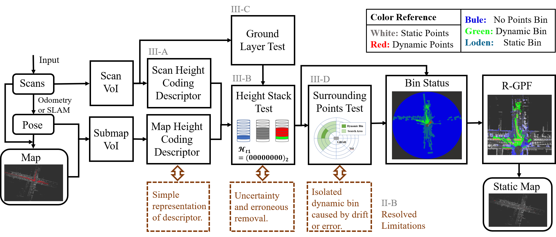
In this paper of work, we follow the thought of descriptor-based method ERASOR [3], introduce a novel representation of descriptors, and multiple effective test methods to overcome existing limitations. The framework of our proposed methods is depicted in Fig.1.
The main contributions of our paper are summarized as follows:
-
•
Novel combination and representation of Height Coding Descriptor (HCD), which contains both extreme values and sparse middle values of the Z axis, which enhances the descriptive capabilities.
-
•
Comprehensive Height Stack Test (HST) method for evaluating dynamic bins, which leverages the description of points in the middle height area in HCD and could avoid potential bad dynamic removal issues associated with inadequate information.
-
•
Additional Ground Layer Test (GLT) and Surrounding Points Test (SPT) for accuracy of dynamic status, which both serve to complement the algorithm and address specific challenges.
-
•
Superior performance compared with the previous work. We compared our proposed ERASOR++ method with the previous ERASOR [3] method, showing that our proposed method outperforms the previous work on both precision and efficiency.
The rest of this paper contains Related Works indicated in Section II, Methodology in ERASOR++ described in Section III, Experiments discussed in Section IV, as well as Conclusion summarized in Section V.
II Related Works
II-A Dynamic Object Removal Methods
Categories of typical post-processing methods are summarized as follows. Cluster-based [6] [7] or semantic-based [8] [9] methods, which often rely on deep learning networks [15]. These methods typically require point cloud supervised labels for training, which can limit their generalization ability. Voxel-based methods [10] [11] [12] tend to be computationally expensive due to the calculation of misses or hits within each voxel. Visibility-based methods [13] [14] heavily depend on the hypothesis that dynamic objects always appear in front of static objects along a ray, rendering them invalid in scenarios where obstacles obstruct the line of sight between sensors and dynamic objects, or in open environments with few regular static objects.
As for the descriptor-based method like Egocentric RAtio of pSeudo Occupancy-based dynamic object Removal (ERASOR) [3] method, proposed by Lim et al., it leverages vertical column descriptors and could overcome the limitations of above with high running speed and a visibility-free characteristic. But it still has some problems like bad removal in some areas, especially when used in unstructured or vegetational environments as shown in the next part.
II-B Main Works and Limitations in ERASOR
ERASOR method focuses on the problem of dynamic objects post-rejection in a set of generated maps. In that paper, Lim et al. brought egocentric descriptor into dynamic area test and proposed the major work using egocentric descriptor-based method. The main work of ERASOR includes leveraging a representation of points in vertical columns called Region-wise Pseudo Occupancy Descriptor (R-POD), a method called Scan Ratio Test (SRT) to fetch bins with dynamic objects, a static point retrieval method called Region-wise Ground Plane Fitting (R-GPF), and presenting a metrics, especially for static map building tasks. More details about the mentioned work can be found in [3].
Although ERASOR provides a promising performance on dynamic object removal, it still has some limitations, which can be summarized as follows.
-
•
Simple representation of descriptor. In the previous method, the representation of the bin area’s descriptor was simplified to only include the height difference along the Z-axis, which seems a substantial loss of valuable information.
-
•
Uncertainty and erroneous removal in areas with blocked ground. As shown in Fig.3, in some area that contains vegetation far from the scan center, or when buildings are positioned behind other objects, the limited number of scan points within the bin leads to potential inaccuracies in determining the status of the bins.
-
•
Isolated dynamic bin caused by drift or error of LiDAR data. As shown in Fig.4, certain bins may exhibit an isolated dynamic status despite the absence of any dynamic objects in that particular area, which leads to wasted computation and ineffective removal processes.
To deal with these limitations above, we modified the previous method and proposed ERASOR++, an improvement based on a height coding method.
II-C LiDAR Descriptors
LiDAR descriptors have been a considerably vital method to represent numerous 3D point cloud information, used in various 3D applications such as location and registration, which can be divided into two key categories, namely hand-crafted and deep-learning based methods. Focused on the traditional hand-crafted approaches, classification can be made by taking into account the extracted region, such as local, global, and hybrid descriptor [16].
Moreover, there are some global descriptors designed for specific applications, like Scan Context [17] and its expansion method [18] [19], which are primarily designed for loop detection tasks. These descriptors leverage spatial distribution or intensity information within each point block, serving as a source of inspiration for the presentation and description of LiDAR point clouds in this paper.
III Methodology in ERASOR++
In this section, the methodology in ERASOR++ is represented in detail in the following parts. The framework of our ERASOR++ method, as well as the connections between methods and limitations in Section II-B are depicted in Fig.1. The subsequent analysis reveals that each method, addressing a specific limitation, contributes to the optimization of the dynamic object removal system from different perspectives.
III-A Height Coding Descriptor
Raw point clouds obtained from scans and prior maps often contain an overwhelming amount of structural information, making calculations complex and challenging. Hence, it is necessary to simplify the information and adopt a novel method to describe the point cloud in the area of interest. Motivated by [3] [17] [18], we propose a novel approach by integrating the height difference and height encoding information, resulting in the Height Coding Descriptor (HCD) which offers a both concise and informative representation of the point cloud in the region of focus.
When the current scan comes, we first fetch the point cloud within a distance range, then get the submap from the prior map by fetching the point cloud in the same range. The Height Coding Descriptor is based on the fetched point cloud as presented in Fig.2.
Let be the point cloud perceived at time step ; be a point in , i.e., ; and be the points fetched from a specific range, also called Volume of Interest (VoI). Then, can be defined and formulated as:
| (1) | |||
where , and . Note that , and are constant threshold of VoI. This formula limits the maximal radial distance boundary using and the valid height range of VoI using and , which can cut down the number of points to be transformed and avoid the outlier.
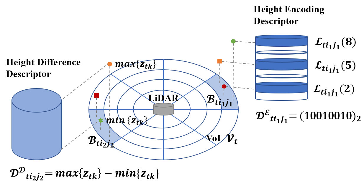
As shown in Fig.2, the VoI will be divided into bins according to azimuthal and radial position, known as sectors and rings. Let be the points of bins in ring and sector, then the points in each bin can be defined as:
| (2) | |||
where , and respectively mean the total divisional numbers of rings and sectors.
In each bin, layer indexes based on height value are utilized to represent the height information in the descriptor. Let be the points in layer index and designed as:
| (3) | |||
where means the total layer number of indexes in each bin.
So the value of Height Coding Descriptor as well as its difference descriptor and encoding descriptor of the bins in ring and sector can be defined as:
| (4) | ||||
| (5) | ||||
| (6) | ||||
| (7) |
Note that the representation of is defined for using bit operation to simplify computation and save storage. As shown in Fig.2, the height occupancy information in each layer can be represented completely using this encoding method with an optional number of total layers , which is always set as 8 or its multiples to match computer storage unit.
Thus, the descriptor can not only show the extreme value of relative height but also represent other points’ height information with a simplified encoding method.
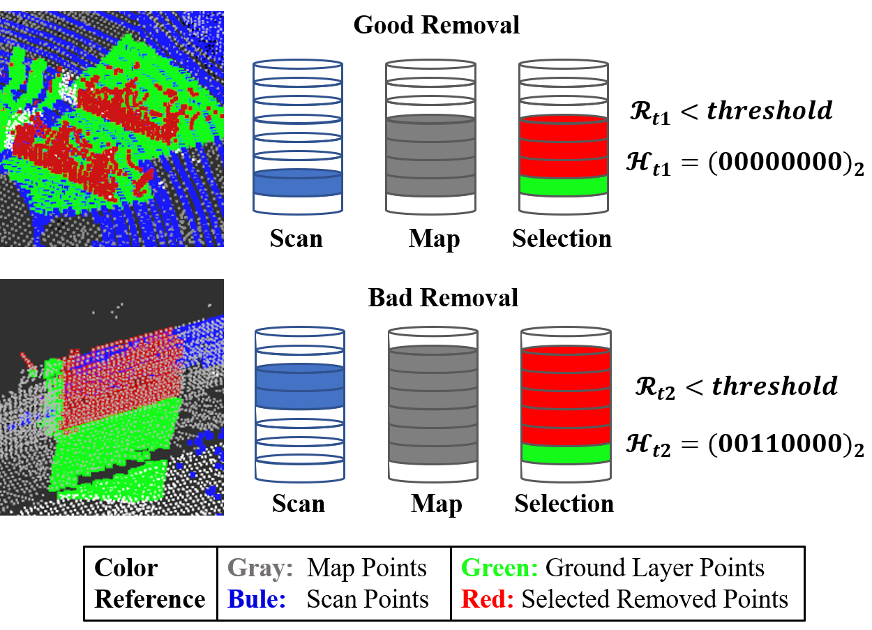
III-B Height Stack Test
In previous work, Scan Ratio Test (SRT) was used to compare the current scan and its corresponding prior map descriptors, in order to found out bins with dynamic objects. SRT directly compares the values of height difference in the current scan and map scan by restricting the quotient of these two values, which can be described as:
| (8) |
which may cause bad removal as displayed in Fig.3. In that case, based on the proposed HCD, a novel test method called Height Stack Test (HST) is designed and utilized.
From Fig.3, we can see that the overlaps in layers above ground need to be checked, and the quantity of overlap parts demonstrates the possibility of being static. So the Height Stack Test parameter is designed as:
| (9) | |||
where the sign and respectively means the AND and NOT operation of bit coding, and means the encoding layer with point cloud below the ground, which is described in the following part III-C. represent overlap layers as well as their position above ground. Note that is always turned to its number of occupied bits to be checked and limited to a low level when coding and implementing.
Thus, with restriction of the position and number of overlap layers, the height information in the middle position can be leveraged, and bad removal caused by blocked points in scan bins can be successfully avoided.
III-C Ground Layer Test
Ground Layer Test (GLT) is a proposed method that involves examining the ground layer within the HCD to determine the relative position for the HST. As the Z direction information of pose from LiDAR Odometry or SLAM is usually more uncertain than X and Y direction [20], the ground layer in each sequence is not united, which causes the necessity of searching ground layer in this system.
From the process above, each point in VoI is related to one bin and can be indexed from the ring number and sector number in . Considering that ground points can always be fetched near the scan sensors, we use the index of each bin to iterate from near to far and get the occupied ring , then check the number of points in each layer of these bins, and finally select the layer with enough most points as the ground layer in . If more than three-quarters of bins in ring achieve the same ground layer , the value of , which encodes layers below the ground, is defined as:
| (10) |
where is the sequence of layers with the satisfied number of ground points in the ring of nearest valid bins.
Thus, the ground layer is found and then the height descriptor can represent both absolute and relative information. Note that different from Ground Plane Fitting (R-GPF) in [3], our Ground Layer Test method only leverages a simple calculation to find the layer with ground points and runs independently before all the processes to give restrictive information for the following HST and R-GPF.
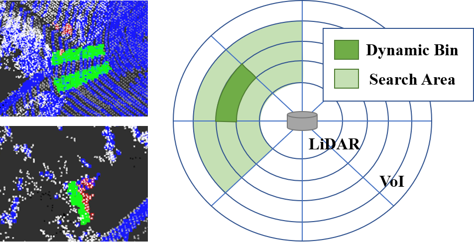
III-D Surrounding Points Test
Surrounding Points Test (SPT) is a process between HST and R-GPF to cut down the wrong dynamic removal. As uncertainty always exists in LiDAR point cloud and some shelters may affect the result of bin status, there are some isolated bins in dynamic status but with no dynamic object in it, as shown in Fig.4.
This part focuses on correcting isolated bin status by searching for neighboring points, aiming to identify and rectify situations where a bin appears to be dynamic due to insufficient surrounding information. By analyzing points in the vicinity, this test ensures a more accurate assessment of the bin’s dynamic status.
For the prior map is generated by the accumulation of each scan frame, dynamic objects always have long tracks in maps. So the bins indeed with dynamic objects should be congregated as groups or lines. Under this circumstance, we proposed the Surrounding Points Test method to check each dynamic bin and make sure their status is right by searching their surrounding points. The search area can be described as:
| (11) | |||
where means the point cloud searching range which can be changed according to the data sequence, and is enough for most situations.
If there are dynamic bins in searching areas, the status of the target bin will remain unchanged. On the contrary, if there are no dynamic bins in searching areas, the status of the target bin will be changed to static status.
Thus, the isolated wrong removal is decreased and more static points are reserved in the output map with an increase in preservation rate.
IV Experiments and Discussion
In this section, we evaluate our proposed dynamic object removal system through comparison and ablation experiments. All the experiments were conducted on a PC with 2.2GHz cores, 16GB RAM, and Robot Operating System (ROS) [21] running in Ubuntu 18.04. The following parts present details of all the experiments.
IV-A Settings and Datasets
Two parts of experiments were set to evaluate and compare the proposed algorithm, including overall system tests and ablation experiments. Overall system tests evaluated the precision and speed of the system with all methods proposed above, while ablation experiments evaluated the effect of partial methods. The initial ERASOR [3] was tested in all datasets for comparison.
According to the system framework in Fig.1, the HCD and GLT parts are preconditions of HST, and SPT can be solely added in ERASOR [3]. So the ablation experiments include the evaluation of system without HCD, GLT, and HST (in Section III-A, III-C and III-B) and system without SPT (in Section III-D). Note that they were respectively named as ++ w/o ABC and ++ w/o D in Table I.
The SemanticKITTI dataset [22] [23] was chosen for experiments, as it provides annotations for each point and labels the ground-truth dynamic objects that need to be removed, which is feasible for us to evaluate the algorithm system. Similar to the datasets used in ERASOR [3], we used the selected frames with the largest part of dynamic object in different sequences, that is, 4390-4530 frames in sequence 00, 150-250 frames in sequence 01, 860-950 frames in sequence 02, 2350-2670 frames in sequence 05, and 630-820 frames in sequence 07.
IV-B Algorithm Precision
Algorithm precision was measured through the novel static map-oriented quantitative metrics in [3] called Preservation Rate (PR) and Rejection Rate (RR).
| Seq. | Method | PR[%] | RR[%] | F1 score | Avg. Time[s] |
|---|---|---|---|---|---|
| 00 | ERASOR | 92.1498 | 97.206 | 0.946104 | 0.125032 |
| ERASOR++ | 96.8261 | 96.1009 | 0.964621 | 0.124875 | |
| ++ w/o ABC | 95.8274 | 96.0592 | 0.959432 | 0.115372 | |
| ++ w/o D | 93.5736 | 96.789 | 0.951542 | 0.135319 | |
| 01 | ERASOR | 91.8967 | 94.5626 | 0.932106 | 0.132209 |
| ERASOR++ | 98.9919 | 93.6401 | 0.962471 | 0.13711 | |
| ++ w/o ABC | 97.3527 | 93.8679 | 0.955785 | 0.126481 | |
| ++ w/o D | 94.9805 | 94.139 | 0.945579 | 0.143876 | |
| 02 | ERASOR | 80.896 | 99.2045 | 0.891197 | 0.161044 |
| ERASOR++ | 87.8949 | 98.9015 | 0.930739 | 0.135772 | |
| ++ w/o ABC | 82.6932 | 99.2045 | 0.901995 | 0.154411 | |
| ++ w/o D | 85.9189 | 98.9015 | 0.919542 | 0.13935 | |
| 05 | ERASOR | 86.9621 | 97.9208 | 0.921167 | 0.121533 |
| ERASOR++ | 96.5283 | 97.6666 | 0.970941 | 0.10012 | |
| ++ w/o ABC | 91.2505 | 97.7049 | 0.943673 | 0.113161 | |
| ++ w/o D | 94.4625 | 98.1019 | 0.962478 | 0.10433 | |
| 07 | ERASOR | 93.4848 | 98.8887 | 0.961109 | 0.090536 |
| ERASOR++ | 98.5774 | 98.6509 | 0.986141 | 0.101062 | |
| ++ w/o ABC | 96.6388 | 98.768 | 0.976918 | 0.088366 | |
| ++ w/o D | 97.583 | 98.6935 | 0.981351 | 0.105337 |
PR describes the effect of static point cloud preservation as an evaluation of bad removal, which is the ratio of the preserved static points in all static points. RR describes the effect of dynamic point cloud removal, which is the ratio of removed dynamic points in all dynamic points. Both of these metrics were calculated voxel-wise with a voxel size of 0.2. score is the combination metric of PR and RR.
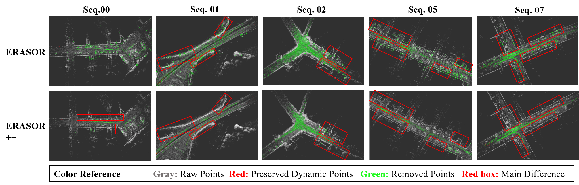
The results of the previous and proposed algorithm as well as the ablation experiments are listed in Table I, in which the previous algorithm was replicated using its open source code. The visual comparison of results with main differences in red boxes is depicted in Fig.5, which provides a clear representation of the effectiveness of the algorithm. It is shown that in all sequences, our method consistently achieves extreme improvements in Preservation Rate and F1 score, with only a slight decrease in RR value. And Preservation Rate in our method can always be kept at a high level. Although in sequence 02, there is a defective PR caused by the pose uncertainty in the Z axis, the results still greatly outperform the previous work. Moreover, considering the difference in points quantity, the improvement in the preserved static points number by our algorithm far outweighs the changes in the dynamic points number.
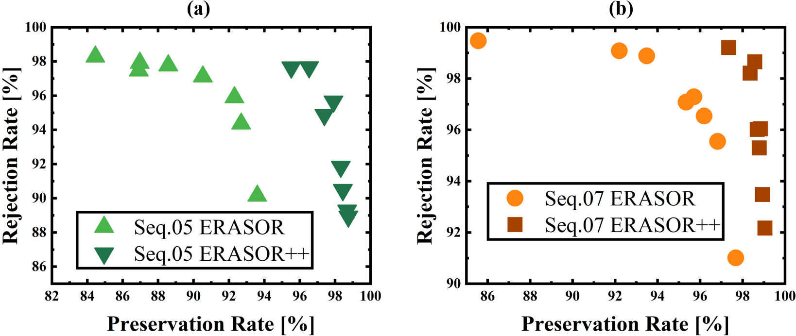
Note that when testing in long-term datasets, there is no need to run the dynamic removal system in each frame. As an external parameter, the frame skip interval could also influence the PR and RR values of each method. We tested and compared these two methods with different interval parameters, and the results of sequences 05 and 07 are depicted in Fig.6. It shows that through the trend of PR-RR relationship, the results of ERASOR++ always display on the high-value side and win high-level precision compared with ERASOR.
That is, our proposed algorithm demonstrates superior precision compared to the previous ERASOR [3] algorithm across various sequences.
IV-C Algorithm Speed
| Method | Seq. 05 | Seq.07 | ||
|---|---|---|---|---|
| Average Eva. | R-GPF Count | Time[s] | R-GPF Count | Time[s] |
| ERASOR | 577.9 | 0.121533 | 531.632 | 0.090536 |
| ERASOR++ | 368.875 | 0.10012 | 390.053 | 0.101062 |
Algorithm speed was measured through the average time taken for one frame iteration during the execution of the main algorithm. We also compared the speed of our proposed method with the previous ERASOR work and other ablation systems, as shown in Table I.
On account of the main time-costing calculation part R-GPF, the count of this part decides the time cost of algorithms. As shown in Table II, although our proposed methods have some incremental calculations compared with the previous method, our algorithm demonstrates an equivalent or even faster execution time compared to the previous ERASOR algorithm, for the iteration counts of R-GPF are less than ERASOR methods. Considering that the previous ERASOR algorithm is already known to be at least ten times faster than other methods [3], our proposed algorithm, ERASOR++, also achieves a comparable level of efficiency.
This indicates that our algorithm not only improves upon the previous algorithm in terms of accuracy and precision but also maintains a comparable level of speed performance.
IV-D Ablation Experiments
The results of ablation experiments are listed in Table I. From all the experiment sequences, the results of our system without each part demonstrate a decrease in Preservation Rate, which means these parts can avoid different kinds of bad removal and solve corresponding limitations.
Through these ablation experiments, the validation of each part can be proved. The Surrounding Points Test and Height Coding Descriptor as well as its corresponding test methods effectively decrease the bad removal and improve the system generalization.
V Conclusions
In this work, an improved dynamic object removal system ERASOR++ was proposed. Building upon the previous work of ERASOR [3], our method introduced a novel representation called Height Coding Descriptor, along with the comprehensive Height Stack Test, Ground Layer Test, and Surrounding Points Test. The proposed system addressed the limitations of ERASOR and effectively promoted the quality of preserved static points with total structure, particularly in unstructured environments, which can greatly contribute to map reconstruction. This improvement offers a more accurate and robust alternative for dynamic object removal when constructing static maps.
In future works, with the innovation of novel representation, the descriptor is supposed to be completed through more available information from raw point clouds, and further, be utilized in other challenging tasks or aspects, providing further opportunities for exploration and utilization.
Acknowledgments
This work was supported by STI 2030-Major Projects 2021ZD0201403, in part by NSFC 62088101 Autonomous Intelligent Unmanned Systems.
References
- [1] H. Yin, X. Xu, S. Lu, X. Chen, R. Xiong, S. Shen, C. Stachniss, and Y. Wang, “A survey on global LiDAR localization,” arXiv preprint arXiv:2302.07433, 2023.
- [2] I. Kostavelis and A. Gasteratos, “Semantic mapping for mobile robotics tasks: A survey,” Robotics and Autonomous Systems, vol. 66, pp. 86–103, 2015.
- [3] H. Lim, S. Hwang, and H. Myung, “ERASOR: Egocentric ratio of pseudo occupancy-based dynamic object removal for static 3D point cloud map building,” IEEE Robotics and Automation Letters, vol. 6, no. 2, pp. 2272–2279, 2021.
- [4] D. Yoon, T. Tang, and T. Barfoot, “Mapless online detection of dynamic objects in 3D LiDAR,” in 2019 16th Conference on Computer and Robot Vision (CRV), 2019, pp. 113–120.
- [5] T. Fan, B. Shen, H. Chen, W. Zhang, and J. Pan, “DynamicFilter: an online dynamic objects removal framework for highly dynamic environments,” in 2022 International Conference on Robotics and Automation (ICRA), 2022, pp. 7988–7994.
- [6] P. Pfreundschuh, H. F. Hendrikx, V. Reijgwart, R. Dubé, R. Siegwart, and A. Cramariuc, “Dynamic object aware LiDAR SLAM based on automatic generation of training data,” in 2021 IEEE International Conference on Robotics and Automation (ICRA), 2021, pp. 11 641–11 647.
- [7] P. Ruchti and W. Burgard, “Mapping with dynamic-object probabilities calculated from single 3D range scans,” in 2018 IEEE International Conference on Robotics and Automation (ICRA), 2018, pp. 6331–6336.
- [8] A. Milioto, I. Vizzo, J. Behley, and C. Stachniss, “RangeNet ++: Fast and accurate lidar semantic segmentation,” in 2019 IEEE/RSJ International Conference on Intelligent Robots and Systems (IROS), 2019, pp. 4213–4220.
- [9] L. Sun, Z. Yan, A. Zaganidis, C. Zhao, and T. Duckett, “Recurrent-OctoMap: Learning state-based map refinement for long-term semantic mapping with 3-D-LiDAR data,” IEEE Robotics and Automation Letters, vol. 3, no. 4, pp. 3749–3756, 2018.
- [10] S. Pagad, D. Agarwal, S. Narayanan, K. Rangan, H. Kim, and G. Yalla, “Robust method for removing dynamic objects from point clouds,” in 2020 IEEE International Conference on Robotics and Automation (ICRA), 2020, pp. 10 765–10 771.
- [11] J. Schauer and A. Nüchter, “The Peopleremover—removing dynamic objects from 3-D point cloud data by traversing a voxel occupancy grid,” IEEE Robotics and Automation Letters, vol. 3, no. 3, pp. 1679–1686, 2018.
- [12] A. Hornung, K. M. Wurm, M. Bennewitz, C. Stachniss, and W. Burgard, “Octomap: An efficient probabilistic 3d mapping framework based on octrees,” Autonomous robots, vol. 34, pp. 189–206, 2013.
- [13] G. Kim and A. Kim, “Remove, then revert: Static point cloud map construction using multiresolution range images,” in 2020 IEEE/RSJ International Conference on Intelligent Robots and Systems (IROS), 2020, pp. 10 758–10 765.
- [14] F. Pomerleau, P. Krüsi, F. Colas, P. Furgale, and R. Siegwart, “Long-term 3D map maintenance in dynamic environments,” in 2014 IEEE International Conference on Robotics and Automation (ICRA), 2014, pp. 3712–3719.
- [15] X. Chen, S. Li, B. Mersch, L. Wiesmann, J. Gall, J. Behley, and C. Stachniss, “Moving object segmentation in 3d lidar data: A learning-based approach exploiting sequential data,” IEEE Robotics and Automation Letters, vol. 6, no. 4, pp. 6529–6536, 2021.
- [16] X.-F. Han, S. Sun, X. Song, and G. Q. Xiao, “3D point cloud descriptors in hand-crafted and deep learning age: State-of-the-art.” arXiv: Computer Vision and Pattern Recognition, 2018.
- [17] G. Kim and A. Kim, “Scan Context: Egocentric spatial descriptor for place recognition within 3D point cloud map,” in 2018 IEEE/RSJ International Conference on Intelligent Robots and Systems (IROS), 2018, pp. 4802–4809.
- [18] Y. Wang, Z. Sun, C.-Z. Xu, S. E. Sarma, J. Yang, and H. Kong, “LiDAR Iris for loop-closure detection,” in 2020 IEEE/RSJ International Conference on Intelligent Robots and Systems (IROS), 2020, pp. 5769–5775.
- [19] H. Wang, C. Wang, and L. Xie, “Intensity Scan Context: Coding intensity and geometry relations for loop closure detection,” in 2020 IEEE International Conference on Robotics and Automation (ICRA), 2020, pp. 2095–2101.
- [20] J. Zhang and S. Singh, “LOAM: LiDAR odometry and mapping in real-time.” in Robotics: Science and Systems, vol. 2, no. 9. Berkeley, CA, 2014, pp. 1–9.
- [21] M. Quigley, K. Conley, B. Gerkey, J. Faust, T. Foote, J. Leibs, R. Wheeler, A. Y. Ng et al., “ROS: an open-source robot operating system,” in ICRA workshop on open source software, vol. 3, no. 3.2. Kobe, Japan, 2009, p. 5.
- [22] J. Behley, M. Garbade, A. Milioto, J. Quenzel, S. Behnke, C. Stachniss, and J. Gall, “SemanticKITTI: A dataset for semantic scene understanding of LiDAR sequences,” in 2019 IEEE/CVF International Conference on Computer Vision (ICCV), 2019, pp. 9296–9306.
- [23] A. Geiger, P. Lenz, and R. Urtasun, “Are we ready for autonomous driving? the KITTI vision benchmark suite,” in 2012 IEEE Conference on Computer Vision and Pattern Recognition, 2012, pp. 3354–3361.