Equivalence relations and distances between time series with application to the Black Summer Australian bushfires
Abstract
This paper introduces a new framework of algebraic equivalence relations between time series and new distance metrics between them, then applies these to investigate the Australian “Black Summer” bushfire season of 2019-2020. First, we introduce a general framework for defining equivalence between time series, heuristically intended to be equivalent if they differ only up to noise. Our first specific implementation is based on using change point algorithms and comparing statistical quantities such as mean or variance in stationary segments. We thus derive the existence of such equivalence relations on the space of time series, such that the quotient spaces can be equipped with a metrizable topology. Next, we illustrate specifically how to define and compute such distances among a collection of time series and perform clustering and additional analysis thereon. Then, we apply these insights to analyze air quality data across New South Wales, Australia, during the 2019-2020 bushfires. There, we investigate structural similarity with respect to this data and identify locations that were impacted anonymously by the fires relative to their location. This may have implications regarding the appropriate management of resources to avoid gaps in the defense against future fires.
keywords:
Bushfires , Time series analysis , Metric spaces , Equivalence relations1 Introduction
We begin with the following general question: can one define equivalence relations between time series, whereby two time series are declared equivalent if they differ only up to noise? This is our guiding heuristic; in this paper, we give one concrete way to understand this.
We begin with motivation: in set theory and throughout mathematics, an equivalence relation on a set can simplify the set. Indeed, an equivalence relation partitions the original set into equivalence classes - subsets of in which everything is mutually equivalent. By considering the set of equivalence classes , equivalent elements of the original have been collapsed or divided down to the same element of ; for this reason, the latter is called the quotient set.
If we wish to understand time series as equivalent if they differ only up to noise, and then wish to define distance measures that “cancel out the noise”, we would like to define equivalence relations such that the quotient set is metrizable, namely can be imbued with an appropriate metric. Then, two equivalence classes of time series and would have an unambiguous distance apart. That is, any time series in the class and any time series in the class would have a noise-invariant distance apart.
To concretely define these equivalence relations, we take the posture that time series consist of locally stationary segments separated by change points (or structural breaks) at which the statistical properties of the time series change, a frequent assumption in the statistical literature [1]. If two time series have the exact same structural breaks and appropriately chosen statistical properties (up to completely identical distributions) in each of the segments, then the difference between them is random noise. This is of course just one way to build a framework envisioned by the paragraphs above.
The following theorem proves that the above goals are possible. Formally, it combines Theorems 2.4 and 2.5:
Theorem 1.1.
There exist equivalence relations on the space of time series, obtained from algorithmic determination of change points, such that the resulting quotient spaces are metrizable. Further, such metrics are continuous with respect to perturbation of the time series.
The proof and construction of such equivalence relations build on several insights: the change point algorithms developed by [2, 3] and [4], the distances between change points of [5], and the construction of Lebesgue spaces as metrizable quotients by [6].
The most significant equivalence relation between functions in measure theory is that of almost everywhere equivalence: define if a.e., that is, is measure zero. We rely on this crucial equivalence relation for both the motivation and mathematics of our theorem and construction.
We recall the construction of the spaces. Let be the vector space of all Lebesgue-measurable functions on such that has finite integral. We have a quotient mapping, defined and outlined in [7],
We will use this notation in what follows. One then equips this quotient space with the norms, as defined in [7] or in Section 2 for our specific case.
1.1 Overview of change point detection
Many domains in the physical and social sciences are interested in the identification of change points/structural breaks in time series data. Introduced by [2] and developed further by [3, 8], change point algorithms are an evolving field of algorithms intended to determine such breaks at change points, when a change in the statistical properties of a time series has occurred.
In the statistical literature, focused on time series data, researchers have developed change point models driven by hypothesis tests, where -values allow scientists to quantify the confidence in their algorithms [9, 10, 11]. Change point algorithms generally fall within Bayesian or hypothesis testing frameworks. Bayesian change point algorithms [12, 13, 14, 15] identify change point in a probabilistic manner and allow for subjectivity through the selection of prior distributions, but suffer from hyperparameter sensitivity and do not provide statistical error bounds or -values, often leading to a lack of reliability.
Within hypothesis testing, [16] outlines algorithmic developments in various change point models initially proposed by [2]. Some of the more important developments in recent years include the work of [3] and [17, 18, 4]. Ross [16] recently introduced the CPM package, which allows for flexible implementation of various change point models on time series data. Given the package’s flexibility and efficient implementation, we build our methodology on this suite of algorithms.
There are also alternative approaches to change point analysis outside the statistical literature. For example, [19] assigns to a time series a change point score that changes with time. Specifically, it measures the dissimilarity of the span of future sequential vectors of time series data with sequential vectors of past data, using matrix algebra.
1.2 Overview of distance measures
The application of metric spaces has provided the groundwork for research advancement in numerous fields. Within time series analysis, new applications of metrics between time series have been found by various authors [20, 21, 22, 23, 24, 25, 26]. Outside time series, the use of metrics has become a popular topic within the field of both statistics and machine learning, where a distance function is optimally tuned for a candidate task. There have been numerous applications, including computer vision [27, 28], text analysis [29, 30], program analysis [31] and many others [32, 33, 34, 35, 36].
Numerous areas of research have found it fruitful to consider more general implementations of distance functions and measures, such as semi-metrics. Within time series analysis, Aßfalg et al. [37] use metrics restricted to particular time intervals to focus on discrepancy at key times, as may be informed by the field of application. The same authors develop a framework of “threshold query execution”, where they restrict time series to unbroken intervals consistently above a certain cutoff threshold , and may then measure distances based on the length and location of these threshold intervals [38, 39, 40], also proposing ways to best select [41]. Batista et al. give an overview of measures between time series and various desirable properties of invariance they may have [42]. In particular, they introduce a new complexity-adjusted distance between time series designed to satisfy a property of complexity-invariance. They take an elegant approach that simply multiplies the Euclidean metric between two time series by an ordered ratio of the time series’ complexities, producing a semi-metric that satisfies a -adjusted form of the triangle inequality. Too many authors to list have used dynamic time warping (DTW) between time series [43, 44, 45, 46, 47, 48], with numerous authors proposing highly efficient means to speed up the algorithm [49, 50].
Outside time series analysis, semi-metrics have proven particularly useful to measure discrepancy between sets of points, and have applications in image analysis [51, 52, 53], fuzzy sets [54, 55, 53, 56] and improved computation in such tasks [57, 58, 59, 60]. An overview of such applications is given by [61].
In our previous work [5], we conduct a computational analysis of various existing metrics and semi-metrics between finite sets, both the traditional metrics such as Hausdorff and Wasserstein, and the more recently introduced semi-metrics used in applications above. We also develop a new semi-metric between finite sets, show some desirable properties compared to existing options, and apply this to measuring distance between time series’ sets of structural breaks. Our methodology has two downsides: these semi-metrics do not obey the triangle inequality, and the distance computation does not record any of the time series’ attributes between these structural breaks. It really reduces entirely from a distance between time series to a semi-metric between sets. Similar work has been undertaken among some of the aforementioned authors, but their approaches generally share the same limitations as our previous work. The threshold query execution of Aßfalg et al. [38, 39, 40] may be used to create a distance between time series, but their proposed semi-metric does not use any of the data within the thresholded intervals. While they do not explicitly use it as a distance measure, the score of [19] could be used to compare time series, but would also lose track of the values taken by the time series. And [37] simply uses pre-entered intervals to compare distance, which must be the same for each time series - it does not aim to detect or use structural breaks.
In this paper, we develop new procedures for measuring discrepancy between time series based on structural breaks, simultaneously ameliorating these downsides and proving Theorem 1.1 in the process. We associate to a time series a piecewise constant function that contains the data of the change points as well as the mean, variance, or other desired property, and embed these piecewise constant functions within . This procedure is highly flexible, building upon any available change point algorithm and recording any desired statistical property.
We also incorporate clustering and outlier detection, drawing upon numerous approaches to time series analysis that have been successfully applied in numerous disparate fields such as epidemiology [62, 63, 64, 65, 66, 67, 68], environmental sciences [69, 70, 71], finance [72, 73, 74, 75, 76, 77, 78, 79, 80], cryptocurrencies [81, 82, 83, 84, 85], crime [86, 87, 88], the arts [89, 90], and other fields [91, 92, 93, 94].
1.3 Overview of the Australian bushfires and related environmental science
The 2019-2020 bushfire season in New South Wales (NSW), Australia, attracted international attention. Multiple states of emergency were declared across the state [95, 96], over five million hectares were burned [97], and the NSW Rural Fire Service stated “2019/20 was the most devastating bush fire season in NSW history, truly unparalleled in more ways than one” [98]. Apart from the immediate damage, the bushfires subjected the entire state to poor, and often hazardous, air quality [99, 100, 101, 102], which has been described as unprecedented by several researchers [103, 104]. Even after the pollution subsided, it may have caused significant damage to the ozone layer, causing further health risks [105, 106].
As air quality data is a significant barometer of air pollution health risk and a proxy for the severity of bushfires nearby, we analyze air quality index (AQI) time series data from the New South Wales Department of Planning and Environment [107]. We examine hourly data over a three-month window, October 20, 2019 - January 20, 2020, measured at 52 stations across the state, whose location is also recorded. This period represents the peak of the bushfire season, where poor AQI data was observed rather uniformly across the entire state. Our paper builds on a growing literature of using supervised and unsupervised learning methods to analyze air quality data, including random forest algorithms [108, 109], generalized additive models [110], principal component analysis [111], and non-parametric smoothing [112]. As bushfire events in Australia and elsewhere continue to increase in prevalence and intensity [113], we hope such mathematical analysis of air quality and other data may continue to inform policymakers and the public of the precise dangers of such pollution, and allow informed decision-making and mitigation in advance.
This paper is structured as follows: in Section 2, we construct the equivalence relations, associated quotient spaces, and metrics between time series, and prove all pertinent theorems. In Section 3, we investigate desirable properties of our metrics relative to existing options, by both theoretical propositions and simulation. In Section 4, we describe our methodology for analysis of a collection of time series with our new metrics, including in a cross-contextual setting. In Section 5, we perform our analysis on the NSW air quality index time series. Section 6 summarizes implications of our methodology and the findings regarding bushfires in Australia and elsewhere.
2 Proof of theorems and construction
Let be a real-valued time series over some time interval , and the space of such time series. In this paper, we only record each data series once, so treat each as a single observed real number. Let be the set of finite subsets of . Throughout the paper, is a chosen real number.
First, one selects a statistical attribute, such as mean, variance, or higher-order moment. For simplicity of exposition, we describe the procedure for the mean. We use the two-step algorithm of [16] to determine a set of change points with respect to changes in the mean. This is an inductive deterministic procedure that uses iterated hypothesis testing. At each step, the null hypothesis of no change point existing is tested, and subject to preset parameters, the null hypothesis may be ruled invalid; this determines a change point. In addition, we set . Properly interpreted, this gives a function
| (1) |
Different parameters yield different algorithms and hence different such functions. This procedure has algorithmically determined that has a constant mean over each interval . By using the change point algorithm or simply averaging over these intervals, we compute and record the empirically observed means . Now we define a function
| (2) |
as a weighted indicator function. This is a piecewise constant function that codifies the change points of the time series and its changing means. That is,
| (3) |
Let be the image of under the almost everywhere equivalence relation. This step means that the values of at the change points do not matter, for a finite set of points is measure zero. Let be the subspace of consisting of (the images of) piecewise constant functions. Properly interpreted, our procedure is the function
| (4) |
This defines an equivalence relation on and an embedding
| (5) |
We note that is a vector subspace of and thus inherits its norm , defined by
| (6) |
normalized so that . When , there is an inner product associated to the norm:
| (7) |
At this point we must make some careful definitions and observations. While has a vector space structure, the change point algorithms do not respect addition of time series, and hence is not linear. The absence of linearity forces us to differentiate two separate definitions. First, the metric space structure on induces a metric on and a pseudo-metric on itself. Concretely, if map to piecewise constant functions respectively, define .
Secondly and separately, we can pullback the norm structure to as a measure of the overall magnitude of the time series, defining . We use the symbol mag, rather than , as this is neither a norm nor semi-norm on . Concretely, but That is, mag does not induce the metric Only after passage to , via the non-linear , does the norm induce the metric.
Now we prove that has all properties of a metric on .
Lemma 2.1.
If then , establishing the triangle inequality for .
Proof.
Passing to it suffices to prove for any elements of , This is known as Minkowski’s inequality, [114]. First, the concavity of implies Young’s inequality: if then
| (8) |
Next, one proves Hölder’s inequality:
| (9) |
To prove this, without loss of generality, we can normalize and so that both It remains to prove Young’s inequality gives, for ,
| (10) |
We integrate this to get as required. Finally,
| (11) | ||||
| (12) | ||||
| (13) | ||||
| (14) | ||||
| (15) |
The first inequality is by the triangle inequality, the second is by Hölder. The final equality holds as We divide by , assuming it is non-zero, to get the result. If is zero, the result is trivial. ∎
Lemma 2.2.
Given time series , the following are equivalent:
-
1.
;
-
2.
;
-
3.
have the same set of change points and the same values of means between them.
In particular, equivalence does not depend on the parameter . Figure 1 depicts some examples of equivalent time series.
Proof.
Let and map to and respectively. Condition 3. states that . By definition of , condition 2. states that , while condition 1. states that . Clearly then, 3. implies 2., and 1. and 2. are equivalent since is a norm on Finally, we suppose 1. holds. Then is itself a piecewise linear function with norm zero. If and have breaks and , respectively, then is continuous on . Since the integral of is zero over this region, continuity means is identically zero on . As such, all the open intervals and must coincide, with the exact same coefficients. This proves condition 3. ∎
Lemma 2.3.
Let be time series, and suppose is compared with a perturbation Suppose differs from on an interval such that the change point algorithm detects two additional change points at and a mean that differs by from the mean of . Then
| (16) |
That is, and are continuous with respect to small deformations in the time series. Figure 1 illustrates the suppositions of the lemma.
Proof.
If and map to and , respectively then
| (17) | |||
| (18) | |||
| (19) |
We remark that if then this establishes continuity relative to the length of the deformation interval, in addition to the deformation magnitude. ∎
Combining all these results we have proved the following:

Theorem 2.4 (Mean Theorem).
The space is equipped with a class of functions that induce metrizable quotient spaces . The equivalence can be characterized simply as if and have identical sets of change points and means in their stationary periods, and does not depend on . The metrics are stable under perturbations in the time series. We may also equip with a magnitude function, representing a holistic measure of its changing mean up to noise.
By an identical method, using change point algorithms for changes in variance, one can construct deterministic functions that prove the following:
Theorem 2.5 (Variance Theorem).
is equipped with a class of functions that induce metrizable quotient spaces . The equivalence can be characterized as if and have identical sets of change points and variances in their stationary periods, and does not depend on . The metrics are stable under perturbations in the time series. We may equip with a magnitude function, representing a holistic measure of its changing variance up to noise.
Other statistical properties induce other equivalence relations and maps , all producing variants of Theorem 1.1. There exist change point algorithms that detect changes in all stochastic properties simultaneously; these induce finer equivalence relations.
3 Simulation study and comparison of distances
In this section, we investigate some desirable properties of our metrics relative to existing options, by both theoretical propositions and simulation. First, we briefly compare our new distance to the simple Euclidean distance between time series.
Proposition 3.1.
Let be a mapping induced by a chosen change point algorithm procedure as in Section 2. Let and be two pairs of equivalent time series, that is, . Then . However, regarding the Euclidean metric, the values of and may differ by a linearly increasing function of and .
Heuristically, and differ only up to noise. Our distance filters out the noise and returns the same distance between and as and . However, if the noise between and is “opposite” that of the noise between and , the Euclidean metric may be sensitive to this and add these errors rather than remove them.
Proof.
By definition, and are mapped under to a common element , while and are mapped to a common element . By definition, , concluding the first statement. Now we turn to the Euclidean metric. By the triangle inequality,
| (20) | |||
| (21) | |||
| (22) |
To show this bound can be attained, we suppose while where is “noise” such that and are deemed identical under and analogously for and . Then . For simplicity, assume under the Euclidean inner product that , which would be the case if were locally constant and had mean zero over the locally constant intervals of . Then by the Pythagorean theorem,
| (23) | |||
| (24) | |||
| (25) | |||
| (26) |
which may increase linearly with when it is a linear proportion of , completing the proof. ∎
Next, we examine the performance of our metrics relative to previously proposed such distances between time series based on structural breaks. Our previous work [5] uses metrics and semi-metrics between the sets of change points to measure distance between time series; that work does so without using data of the mean or variance between these breaks. The following simulation study and proposition provide justification for why the distance may more appropriately measure distance between time series.
For this simulation study, we will make use of the following (semi)-metrics between finite sets and . First, let
| (27) |
Then, let the Hausdorff metric be defined as
| (28) | |||||
| (29) |
The modified Hausdorff semi-metric is defined as
| (30) |
The new family of semi-metrics introduced in [5] is defined by
| (31) |
These aforementioned (semi-)metrics between finite sets can readily be applied to measure distance between time series with respect to their change points. If and are time series with change point sets , respectively (under some change point algorithm), one can simply set to be any of or


We generate ten synthetic time series (labeled TS1 - TS10), which we display in Figure 2. These provide example where two different structural breaks (change points) may have markedly different changes in the mean. Black vertical lines indicate detected change points, with the orange line representing the piecewise constant functions . When considering only structural breaks, the most similar time series are groups as follows: {TS1, TS2, TS3}, {TS4, TS5}, {TS6, TS7}, {TS8, TS9, TS10}. However, considering structural breaks and their mean, using our metric induced from , the most similar time series are {TS1, TS3} and {TS7, TS8}.
In Figure 3, we implement hierarchical clustering on the ten synthetic time series with our new metric, here with , as well as existing distance measures in [5]. We see that only the metric, in Figure 3(d), appropriately clusters similar time series according to their changing values, while the other three figures identify erroneous similarities between the time series based solely on their structural breaks. That is, the other (semi-)metrics neglect the additional data that recognizes, demonstrating the superior performance of the latter.
Next, we prove a proposition that demonstrates that only our new metrics are continuous with respect to small deformations in the time series that may introduce new structural breaks. That is, the existing distance measures between change points may be excessively sensitive to new structural breaks, either caused by a deformation in the time series data or a faulty detection by a change point algorithm. We adopt the same suppositions of Lemma 2.3, illustrated in Figure 1.
Proposition 3.2.
Let be time series, and suppose is compared with a perturbation Suppose differs from on an interval such that the change point algorithm detects two additional change points at and a mean that differs by from the mean of . The three (semi)-metrics between sets are not continuous with respect to deformations in the time series.
Proof.
Adopting the notation of Lemma 2.3, let have structural breaks and respectively. Relative to , has two additional structural breaks . If we measure distance between time series purely relative to structural breaks using the Hausdorff metric , then the distance between and is defined as while that between and is . As such, is constant and non-zero relative to . Hence, it does not approach zero as . The same holds for and .
Moreover, these metrics are not continuous relative to either. Consider the simple case where . Assume . Then . This is also constant relative to and does not approach zero as . A similar argument holds for . This proves the result. ∎
Next, we prove a property that establishes a form of linearity for the metrics analogous to the Euclidean metric or other classical metrics.
Proposition 3.3.
Let be time series and be constants. Suppose the mapping has one of two properties: either
| (32) | |||
| (33) |
Then . That is, respects linear operations between time series.
The proof of this proposition is quite trivial, but understanding the primary condition is more interesting. The property that really has two components: first, that the change points of are the same as , assuming , and secondly, that the statistical quantity is measuring scales commutes with scalar multiplication and the addition of constants. The property (33) has a near-identical interpretation. The former component is more subtle than it looks, relying on the fact that the change point algorithm use normalized test statistics. Fortunately, it is the case that essentially all change point algorithms do use normalized test statistics (and should!) so that means this condition holds for all procedures we will use. As for the latter component, the property (32) holds for the mean and hence of Theorem 2.4. This is simply due to the fact that the mean of a random variable satisfies . On the other hand, the property (33) holds for the standard deviation and hence closely related to of Theorem 2.5. This is also simply due to the fact that .
Proof.
The explanation above and the simple proof show that this proposition applies to the mean-mapping and associated distances of Theorem 2.4 as well the standard deviation-mapping , related to the variance-mapping of Theorem 2.5. That is, respect linear operations between time series (scalar multiplication and the addition of a constant) for both mean and standard deviation.
We conclude this section by considering several invariances our metrics do and do not have, and some modifications one may make for a desired application. First, Proposition 3.1 immediately establishes noise-invariance, when properly defined, the guiding property of the entire framework. Next, as a result of Proposition 3.3, are not invariant to amplitude (caling ) or offset in the -direction (when is left invariant but ). However, both of these invariances can be attained by simply normalizing the time series prior to analysis (computing Z-scores) as required by the application. This is required in most domains [50, 42], and in fact we do perform such a normalization when computing normalized distances in Section 4.
Other invariances must be established by modifying our distances, which should be possible by combining with existing approaches. For example, [42] elegantly multiply the Euclidean metric by an ordered ratio of the complexities of two time series to establish a complexity-invariant distance. That approach should work analogously for our metrics. Phase invariance is a complex problem, for which typically the best approach is testing all possible alignments [45, 115]. A similar problem exists for (global) warping, namely (uniform) scaling in the -direction: one must test all possibilities within a given range [43]. Such approaches could be incorporated for our distances.
4 Methodology
In this section, we describe a general procedure to use the function and the induced distances to compute and analyze distances in a collection of time series. We will subsequently apply this procedure to analyze the Australian bushfires in the next section. Suppose are time series over some time period . We suppress the time in our notation.
First, we choose an appropriate change point algorithm for the data, including threshold parameters, and a desired statistical quantity, such as mean or variance. This specifies a precise instance of . Let the piecewise constant functions associated to the time series be , so that . Also, we consider the normalized piecewise constant functions . We form three different matrices:
| (34) | |||
| (35) | |||
| (36) |
Remark 4.1.
We recall . Thus, the normalized are produced by dividing by the aforementioned time series’ magnitude functions.
Remark 4.2.
We note a relation between and for . If are two non-zero elements of an inner product space, with normalized elements then
| (37) | |||
| (38) |
Definition 4.1.
Let a and be matrices. Then a termed a distance matrix if is symmetric, for all and . Similarly, is termed an affinity matrix if is symmetric, and
Given a distance matrix one may produce an affinity matrix by:
| (39) |
is a distance matrix, thus named as it consists of unscaled distances. is also a distance matrix, consisting of distances between normalized vectors, again with suppressed from the notation. We refer to as an alignment matrix as it measures angles between the as vectors in an inner product space. We note that all entries of lie in with all diagonal elements equal to To the distance matrices and we associate affinity matrices and , respectively.
4.1 Cross-contextual analysis
In many applications (including that of this paper), a collection of time series has additional structure. Each individual series contains numerical data one can compare with each other, but there may also exist contextual data among the indices . For instance, in our specific analysis in the next section, is a time series of measurements taken at a particular measuring station; the relationships between these stations, such as their physical distance, influences the data. It is of interest to analyze not just the collection of time series, but their relationship with physical distance of these measuring stations, or other cross-contextual data. We introduce a general framework for cross-contextual distance analysis. Let be a distance matrix that codifies relationships between the sources of the data, As above, we can associate an affinity matrix to these distances. Then, define consistency matrices
| (40) | |||
| (41) | |||
| (42) |
These matrices measure the consistency between the affinity measured by our measures on time series, and a cross-contextual distance matrix .
4.2 Clustering and outlier detection
With the definitions of Section 4.1 in mind, we may apply the methods of spectral and hierarchical clustering in two ways. First, as is standard, we may apply it directly to the matrices , to determine anomalies and clusters of similarity with respect to the distance between time series. Because the entries of are obtained as a linear combination of the entries of , clustering with respect to a distance matrix or its associated affinity matrix gives identical results. The same applies for and , by remark 4.2: these will cluster in identical ways.
In addition, we may also apply clustering techniques to the consistency matrices defined above. This will identify those anomalous data sources, indexed by , which do not behave similarly between the two distance measures. In Section 5, we will uncover striking similarity when considering both distances between air quality time series and geographical distances and will identify just a handful of anomalous locations where this relationship does not hold; these are anomalies in the consistency matrix.
Finally, we also compute the matrix norms of the consistency matrices as a measure of the overall consistency between the distance measures. We use the normalized norm
| (43) |
5 Australian bushfire data
In this section, we analyze AQI time series from locations across NSW [107]. Each time series consists of hourly data from October 20, 2019 - January 20, 2020, to yield time series of length . In the rare case of missing data points, we take the value from the most recent prior hour. We record latitudes and longitudes of the measurement stations, from which we compute the matrix of geographical distances using the Haversine formula [116].
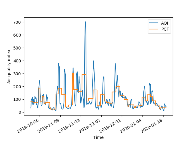
Mathematically, this data is a suitable opportunity to apply our metrics derived from distances between piecewise constant functions generated from change point algorithms. The change point procedure helps stabilize the data more appropriately, measuring average air quality over intervals of days rather than the huge peaks seen in the raw AQI time series. Since we expect air quality to remain somewhat locally stationary, these change point algorithms are more appropriate than more flexible but less targeted non-parametric models.
Within this multivariate context, we perform two separate analyses. First, our new distance matrices, computed according to the algorithmic framework of Section 2, enables the identification of similarity clusters and anomalies. Second, calculating the geographical distances between measuring sites gives a contextual distance matrix . As described in Section 4, we may form associated consistency matrices. With each of these matrices, we apply hierarchical and spectral clustering, thereby identifying anomalies in the spread of poor air relative to space and time.
Henceforth, we set .
5.1 Raw AQI data
In Figure 4, we display the raw AQI time series data for select measuring stations across NSW, and perform our algorithm to fit piecewise constant functions for each via , as specified in Section 2. Our results are consistent with geographical proximity and provide several preliminary insights regarding anomalous air quality relative to space and time during our period of analysis. A large number of these measurement sites are located in the city of Sydney, and hence close relative to the rest of the state of NSW. For instance, Randwick and Rozelle are two sites within Sydney that are particularly geographically close geographically, approximately 10 km apart. Figures 4(a) and 4(b) illustrate the striking similarity between these air quality time series. The other four sites will be relevant in subsequent analysis. In Figure 4(c), we note that Narrabri air quality was consistently poor from early November 2019. Wagga Wagga, Katoomba, and Albury, displayed in Figures 4(d), 4(e), and 4(f), all suffered sharp peaks in poor air quality much later than Narrabri. Albury in particular exhibits peaks in poor air quality as late as mid January 2020. Indeed, Albury, on the southern border of NSW, was affected by the fires much later, as they moved south. Curiously, we see that the two Sydney-based stations, Randwick and Rozelle, exhibited rather moderate levels of pollution from mid-December onward, while Katoomba, located nearby, experienced its most severe air quality.


5.2 Affinity matrix analysis
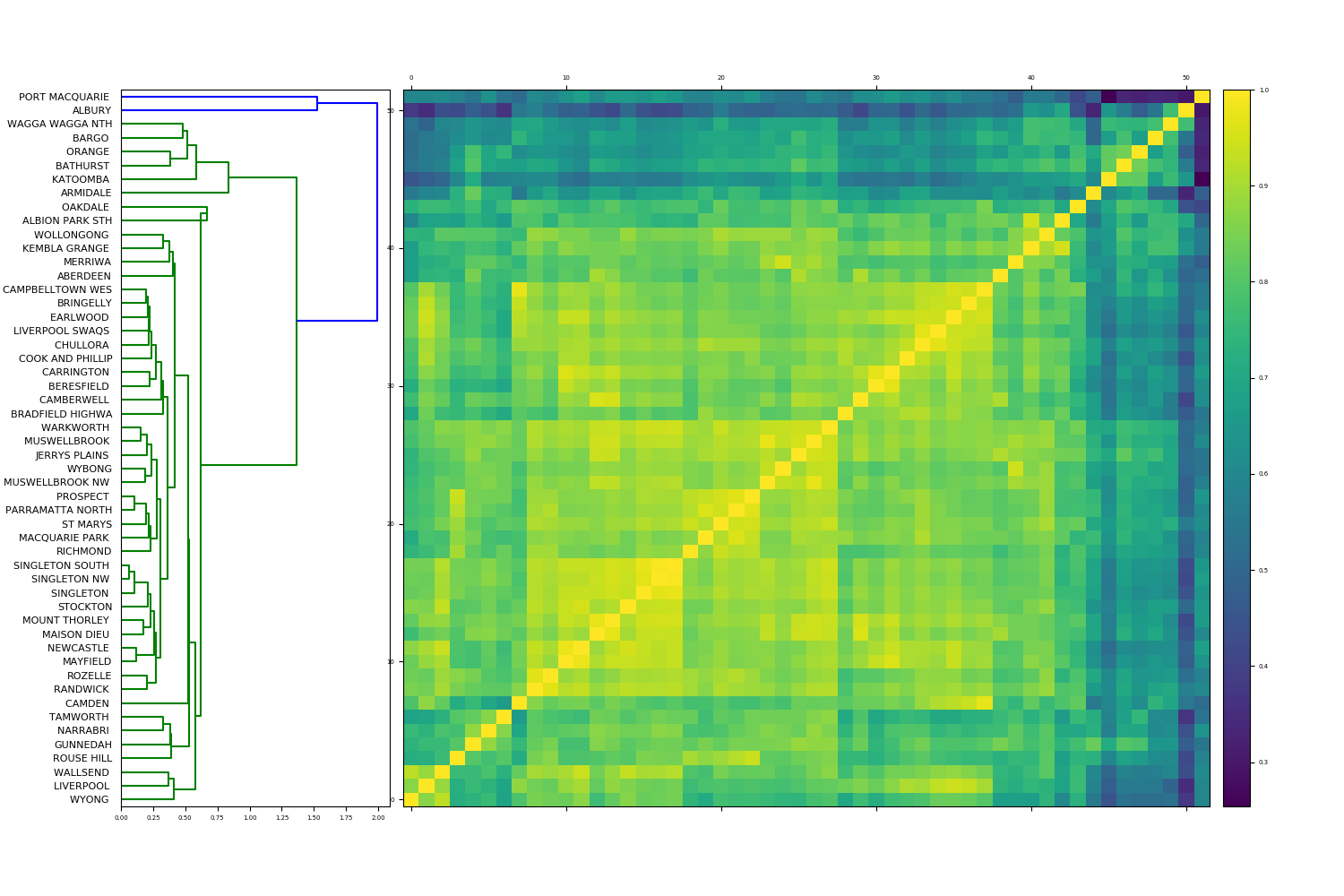
In this section, we use our new distance measures, via the function , to produce clusters of similarity and anomalies with respect to the air quality of different locations. As remarked in Section 4.2, there is no difference between clustering on a distance matrix or its affinity matrix, so we cluster based on affinity matrices and . These entries lie in so that diagrams display a consistent scale. These matrices each provide interesting insights, and are largely consistent with respect to their identification of similarity clusters and anomalies.


| Measuring station | Time series magnitude | Measuring station | Time series magnitude |
|---|---|---|---|
| Aberdeen | 112.1 | Mount Thorley | 122.2 |
| Albion Park | 89.3 | Muswellbrook | 126.0 |
| Albury | 175.2 | Muswellbrook NW | 125.5 |
| Armidale | 195.5 | Narrabri | 105.7 |
| Bargo | 152.7 | Newcastle | 112.8 |
| Bathurst | 181.9 | Oakdale | 196.6 |
| Beresfield | 110.4 | Orange | 204.2 |
| Bradfield Highway | 104.5 | Parramatta North | 116.1 |
| Bringelly | 125.6 | Port Macquarie | 202.0 |
| Camberwell | 139.0 | Prospect | 123.9 |
| Camden | 140.9 | Randwick | 104.6 |
| Campbelltown West | 123.5 | Richmond | 137.7 |
| Carrington | 107.0 | Rouse Hill | 131.2 |
| Chullora | 108.9 | Rozelle | 102.9 |
| Cook and Phillip | 100.7 | Singleton | 116.9 |
| Earlwood | 103.0 | Singleton NW | 116.5 |
| Gunnedah | 104.6 | Singleton South | 113.0 |
| Jerrys Plains | 131.3 | St Marys | 121.4 |
| Katoomba | 258.4 | Stockton | 133.2 |
| Kembla Grange | 97.7 | Tamworth | 159.8 |
| Liverpool | 116.3 | Wagga Wagga North | 174.7 |
| Liverpool Swaqs | 121.8 | Wallsend | 100.0 |
| Macquarie Park | 105.1 | Warkworth | 133.5 |
| Maison Dieu | 140.7 | Wollongong | 98.7 |
| Mayfield | 110.2 | Wybong | 122.7 |
| Merriwa | 133.1 | Wyong | 108.3 |
Figure 5(a) displays hierarchical clustering of , our affinity matrix between unscaled distances. The dendrogram indicates that there is a majority cluster of time series, with two outlier elements, Katoomba and Albury, both of which had marked peaks in poor air quality, confirmed by Figures 4(e) and 4(f). Both areas experienced some of their worst air quality well after other NSW measuring stations, leading to their piecewise constant function being classified as anomalous. The majority cluster contains two subgroups. The first of these is a large subcluster of highly similar time series, containing all Sydney-based measuring stations. The second subcluster consists of less pronounced anomalies, including Armidale, Bargo, Bathurst, Oakdale, Orange, Tamworth, Wagga Wagga (4(d)), and Port Macquarie. All of these locations are “regional locations” located a significant distance from the city of Sydney. Spectral clustering results suggest that there are three clusters: one containing Albury, another containing Katoomba, and the third consisting of the remainder of the time series.
Figure 5(b) depicts , our affinity matrix recording distances between normalized vectors. We have similar results for this matrix. Hierarchical clustering again reveals a large majority cluster, with two outliers, Port Macquarie and Albury. The majority cluster has two subgroups again. One is smaller, consisting of Armidale, Bargo, Bathurst, Katoomba (4(e)), Oakdale, Orange, Tamworth, and Wagga Wagga (4(d)), while the other subgroup contains all remaining locations. In particular, we note that after normalization, Katoomba has left the most anomalous cluster. Indeed, Katoomba is characterized by the single greatest magnitude of all locations, with . We record all time series magnitudes in Table 1. After normalization by the magnitude, recalling Remark 4.1, this extreme feature is nullified. The remainder of the measuring station time series, which again contain all of Sydney, are identified as highly similar. Spectral clustering on the matrix indicates that there are two highly anomalous time series, Port Macquarie and Albury.
Third, we analyze the alignment matrix . Hierarchical clustering is displayed in Figure 5(c). These results are almost identical to the hierarchical clustering on , identifying Port Macquarie and Albury as primary anomalies, and Armidale, Bargo, Bathurst, Katoomba, Oakdale, Orange, Tamworth, and Wagga Wagga as secondary anomalies. The remaining stations, once again containing the entire city of Sydney, are closely clustered. Spectral clustering proposes three clusters of AQI: one cluster containing Port Macquarie, one containing Albury, and one remaining cluster consisting of the remaining locations.
5.3 Cross-contextual analysis
In this section, we analyze the consistency matrices defined in Section 4. These consistency matrices provide a framework for cross-contextual analysis. That is, where one matrix computes the similarity in one aspect, and another matrix computes similarity in a separate aspect, subtracting one affinity matrix from the other allows us to identify the consistency between different similarity measures across a collection of time series. This helps to place measurements between different time series within a greater context. In this instance, we analyze whether air quality is consistent with respect to geographical distance between measuring locations. Anomalies in consistency highlight either a) two areas close by way of geographical distance but dissimilar in air quality or b) two locations far apart in terms of geographical distance, but similar in their air quality.
Hierarchical clustering on the geographical affinity matrix (see Figure 6) determines clusters of measuring stations in terms of their geographical proximity within the collection. A majority cluster is identified with two outliers, Wagga and Wagga, both of which are significantly further south than the other measuring stations. The remaining measuring stations fall in one cluster that appears to have two distinct collections of similarity. The first sub-group contains the city of Sydney sites, while the second sub-group includes locations outside Sydney, both to the west and north.
First, we analyze the consistency matrix associated to the unscaled distance measure, . Hierarchical clustering (Figure 6(a)) indicates a majority cluster with one outlier location, Katoomba. Within the majority cluster there is a small subcluster of anomalous locations including Gunnedah, Narrabri, Albury, Wagga Wagga and others. That is, Katoomba is highly anomalous relative to the relationship between air quality and distance from other locations. Indeed, Katoomba is relatively close to the city of Sydney but was befallen with terrible bushfires close by. Spectral clustering indicates that there are three clusters: the first consisting solely of Katoomba, the second consisting solely of Oakdale and the final cluster containing the remaining measuring locations. The norm of the entire consistency matrix is approximately indicating broad similarity between geographical and AQI affinity.
Next, we consider the consistency matrix associated to the distances between normalized vectors, . The hierarchical clustering results (Figure 6(b)) are highly similar to that of , with a majority cluster detected but Katoomba as a single outlier. Interestingly, there is more variance in the structure of the majority cluster. This demonstrates the utility of our plurality of measurements: others may uncover structure that one alone cannot. Katoomba’s outlier status in this second experiment is by no means obvious and provides another insight: even after normalizing by its extreme magnitude, it is still anomalous relative to the consistency between geographical distance and AQI. Spectral clustering indicates that there are two anomalous locations, Katoomba and Bargo, each of which is contained exclusively within its own cluster. Finally, the matrix norm is , larger than that of . This makes sense given less consistency overall in this matrix.
Finally, we consider the consistency matrix associated to the alignment matrix, . Hierarchical clustering (Figure 6(c)) indicates that there are three clusters of locations. The first is an outlier element, Narrabri, the second cluster consists of Bargo and Katoomba, and the final majority cluster consists of the remaining measurement stations. These can be subcategorized into those located closer to Sydney and those located farther from Sydney. Spectral clustering indicates that the two most anomalous locations are Katoomba and Bargo. Given the reasonable difference in inference generated from each consistency matrix, one can appreciate the importance of using the most appropriate distance measure. The matrix norm is , once again indicating broad similarity. Again, the fact that identifies Narrabri as an outlier while does not demonstrates the utility of our range of measurements, despite the fact that these two distance methods are quite related by Remark 4.2.


6 Conclusion
We have proposed a new theoretical and practical framework for understanding equivalence and computing distances between time series. Mathematically, we aim to identify and quotient by the relation that two time series differ only up to noise, and computationally, we want to remove noise from calculations of distances and magnitudes . Our procedure builds on earlier work to measure distances between time series via sets of structural breaks, and our new method produces more reliable and continuous measures. We have applied the function and these metrics to analyze data with extraordinary peaks, determining piecewise constant functions designed to understand the true movement of the mean (or variance) throughout the time series. This procedure is highly flexible: we could swap variance for mean, vary our change point algorithm parameters, or use completely different change point algorithms altogether.
Several future implementation opportunities exist in this equivalence framework. One could develop and explore notions of weak equivalence if two time series are equivalent under or , and strong equivalence if they are equivalent under both, or more strongly, if they have identical distributions within their change point segments. Moving beyond piecewise constant functions, two autoregressive progresses with the same parameters and could be declared equivalent, if and are each “white noise” variables, namely Gaussian distributions for sufficiently small . Algorithms could be developed to empirically detect such similarity in the distributions from an observed sample set, define equivalence relations, and hence produce reliable distance measures on the induced quotient space. Developing further theoretical and algorithmic ways of determining quotient spaces equipped with metrics may have many applications in determining appropriately adjusted measures between time series. Within a statistical or nonlinear dynamics context, algorithmic frameworks designed to learn appropriate notions of equivalence “up to noise” would also be of great interest to the community. Finally, our distance measures could be incorporated with other advances in distance analysis between time series, such as the search for various different invariances (amplitude, phase, complexity, and others) as discussed at the end of Section 3.
In our analysis of the NSW bushfires, we have determined anomalies not just in the air quality data itself, but also those sites that stand out in the otherwise strong consistency between air quality and geographical distances. By using several different discrepancy matrices, we are able to uncover structure that one alone cannot reveal. Katoomba is a location of particular interest in our analysis. It was initially revealed as highly anomalous in our unscaled distance matrix but less so in the normalized matrix . The initial logical explanation for this is that the feature most anomalous with Katoomba was its considerable scale, reflected in the location’s overall magnitude, the highest among all measuring stations, which is then nullified when normalizing distances are computed in . However, curiously, Katoomba again appears as an outlier in , which uses normalized distances to measure consistency with geographical distance. Examining Katoomba’s time series again (Figure 4(e)) we note that Katoomba experienced its greatest severity in air quality later on in our period of analysis, from mid-December onward, whereas the Sydney stations (which Katoomba is relatively close to) generally experienced severity prior to this.
There is also utility in examining the results of a range of clustering methods. For example, only spectral clustering identifies Oakdale as an anomalous element in its own cluster when considering unscaled distances’ consistency. We have also identified Narrabri as an interesting case. Unlike Katoomba, this location was never identified as a significant anomaly with respect to geography or AQI, considering distances or alignment. And yet, it is anomalous in the consistency between geographical and AQI distances. It is one of very few locations where these two measures are not closely aligned relative to other sites. Indeed, in Figure 4(c) we can see it closely resembles the profile of the Sydney sites despite being quite distant, to the north of the state. In addition, the holistic analysis of various distance and consistency matrices yields several high-level insights. First, there is broad consistency between AQI and geographical affinity matrices, which measure the relationship between sites with respect to these two aspects, as evidenced with the low consistency matrix norms in all implementations. Second, there is clearly sensitivity in the anomalies detected based on the distance measures that are used.
The mathematical analysis of relationships and anomalies between air quality measuring stations could prompt other researchers to conduct closer meteorological or geological examinations of different locations. Such research could shed light on the anomalous nature of Katoomba, Narrabri and other sites discussed in this manuscript. The fact that Sydney’s air quality was much more moderate after mid-December while nearby Katoomba’s became much more severe are too persistent with time to be explained by coincidences such as wind direction, and further exploration of this reasons could provide further insight on how bushfires and air pollution spread. This and other mathematical analysis could encourage researchers to notice hereto-unknown features of the land and its susceptibility or resistance to extreme bushfires, allowing better allocation of resources and understanding of vulnerability to bushfires. As such extreme events increase, we urge more interdisciplinary work between nonlinear dynamics and environmental researchers into such questions.
Data availability statement
The data analyzed in this study are publicly available at [107]. A cached copy is conveniently available at https://github.com/MaxMenzies/BushfireData.
Appendix A Change point algorithm
In this appendix, we describe the specific implementation of the change point detection algorithm used in Sections 4 and 5. The general change point detection framework is as follows: a sequence of observations are drawn from random variables and undergo an unknown number of changes in distribution at . We assume observations are independent and identically distributed between change points, that is, between each change points a random sampling of an underlying distribution is taken. Following [16], we notate this as follows
| (44) |
While the requirement of independence may appear restrictive, dependence can generally be accounted for by several means, such as modelling the underlying dynamics or drift process, then applying a change point algorithm to the model residuals or one-step-ahead prediction errors, as described by [117].
A.1 Batch detection (phase I)
The first phase of change point detection is retrospective. As above, we are given a finite sequence of observations from random variables . For simplicity, we assume there is at most one change point. If a change point exists at time , then observations have some distribution of prior to the change point, and a distribution of proceeding the change point, where . Thus, one must test between the following two hypotheses for each :
| (45) |
| (46) |
and select the most suitable point , if one exists.
One proceeds with a two-sample hypothesis test, where the choice of test depends on assumptions about the underlying distributions. Nonparametric hypothesis tests can be chosen to avoid distributional assumptions. One appropriately chooses a two-sample test statistic and a threshold parameter . If then the null hypothesis is rejected and one provisionally assumes that a change point has occurred at . These test statistics are normalized to have mean and variance and evaluated at all values ; the largest test statistic is assumed to be coincident with the existence of our sole change point. The overall test statistic is then
| (47) |
where are non-normalized statistics.
The null hypothesis of no change point is rejected if for an appropriately chosen threshold . In this case, we conclude that a (single) change point has occurred and its location is the value of that maximizes . That is,
| (48) |
This threshold is chosen to bound the type 1 (false positive) error rate as is commonplace in statistical hypothesis testing. One specifies an acceptable level for the proportion of false positives, the probability of falsely declaring that a change has occurred when in fact it has not. Then, is chosen as the top quantile of the distribution of under the null hypothesis [16].
A.2 Sequential detection (phase II)
In this phase, the sequence does not have a fixed length. New observations are continually received over time, and multiple change points may exist. Assuming no change point exists so far, this phase treats as a fixed-length sequence and computes as described in phase I. A change is detected if for an appropriately chosen threshold. If no change is detected, the next observation is brought into the sequence for consideration and the process continues. If a change is detected, the process restarts from the data point immediately following the detected change point. Thus, the procedure consists of a repeated sequence of hypothesis tests.
In this sequential setting, is selected so that the probability of incurring a Type 1 (false positive) error is constant over time, so that under the null hypothesis of no change point, the following holds:
| (49) | ||||
| (50) |
In this case, assuming that no change point occurs, the expected number of observations received before a false positive detection occurs is . This quantity is known as the average run length, or ARL0 [16].
Appendix B Cluster theory
In this section, we briefly describe the two methods of clustering used throughout this paper. First, hierarchical clustering [118, 119] is an iterative clustering technique that seeks to build a hierarchy of similarity between elements. In this paper we use agglomerative hierarchical clustering with the average linkage method [120], where each element (in our case a location) begins in its own cluster and branches between them are successively built. The results of hierarchical clustering are commonly displayed in dendrograms, as we display in this paper. Unlike spectral or K-means clustering, hierarchical clustering does not specify a discrete partition of elements, and does not require the choice of a number of clusters . Like spectral clustering, hierarchical clustering can be implemented on any distance, not necessarily Euclidean space.
Spectral clustering applies a graph theoretic interpretation of a distance matrix , projecting data into a lower-dimensional space, the eigenvector domain, where it may be more easily separated by standard algorithms such as -means. Following [121], we transform a distance matrix into an affinity matrix as we do throughout the paper (39). Then we define the graph Laplacian by
| (51) |
where is the diagonal degree matrix with diagonal entities and zero off-diagonal entries. and hence are real symmetric matrices, so can be diagonalized with all real eigenvalues (the spectral theorem, [122]). By construction, is positive semi-definite with eigenvalues
Spectral clustering proceeds as follows: with chosen a priori, we find corresponding eigenvectors and construct the matrix whose columns are . Let be the rows of . We apply standard K-means [123] to cluster these rows into clusters . Finally, we determine clusters to assign the original elements into the corresponding clusters. Spectral clustering can be applied for any value of , but a common choice of is to maximize the eigengap between successive eigenvalues .
References
- Dahlhaus [1997] R. Dahlhaus, Fitting time series models to nonstationary processes, The Annals of Statistics 25 (1997) 1–37. doi:10.1214/aos/1034276620.
- Hawkins [1977] D. M. Hawkins, Testing a sequence of observations for a shift in location, Journal of the American Statistical Association 72 (1977) 180–186. doi:10.1080/01621459.1977.10479935.
- Hawkins et al. [2003] D. M. Hawkins, P. Qiu, C. W. Kang, The changepoint model for statistical process control, Journal of Quality Technology 35 (2003) 355–366. doi:10.1080/00224065.2003.11980233.
- Ross [2014] G. J. Ross, Sequential change detection in the presence of unknown parameters, Statistics and Computing 24 (2014) 1017–1030. doi:10.1007/s11222-013-9417-1.
- James et al. [2020] N. James, M. Menzies, L. Azizi, J. Chan, Novel semi-metrics for multivariate change point analysis and anomaly detection, Physica D: Nonlinear Phenomena 412 (2020) 132636. doi:10.1016/j.physd.2020.132636.
- Riesz [1910] F. Riesz, Untersuchungen über systeme integrierbarer funktionen, Mathematische Annalen 69 (1910) 449–497. doi:10.1007/bf01457637.
- Billingsley [1995] P. Billingsley, Probability and Measure, New York: John Wiley Sons, 1995.
- Hawkins and Zamba [2005] D. M. Hawkins, K. D. Zamba, A change-point model for a shift in variance, Journal of Quality Technology 37 (2005) 21–31. doi:10.1080/00224065.2005.11980297.
- Moreno and Neville [2013] S. Moreno, J. Neville, Network hypothesis testing using mixed kronecker product graph models, in: 2013 IEEE 13th International Conference on Data Mining, IEEE, 2013, pp. 1163–1168. doi:10.1109/icdm.2013.165.
- Bridges et al. [2015] R. A. Bridges, J. P. Collins, E. M. Ferragut, J. A. Laska, B. D. Sullivan, Multi-level anomaly detection on time-varying graph data, in: Proceedings of the 2015 IEEE/ACM International Conference on Advances in Social Networks Analysis and Mining 2015, ACM, 2015, pp. 579–583. doi:10.1145/2808797.2809406.
- Peel and Clauset [2015] L. Peel, A. Clauset, Detecting change points in the large-scale structure of evolving networks, in: Proceedings of the Twenty-Ninth AAAI Conference on Artificial Intelligence, AAAI’15, AAAI Press, 2015, p. 2914–2920.
- Barry and Hartigan [1993] D. Barry, J. A. Hartigan, A Bayesian analysis for change point problems, Journal of the American Statistical Association 88 (1993) 309. doi:10.2307/2290726.
- Xuan and Murphy [2007] X. Xuan, K. Murphy, Modeling changing dependency structure in multivariate time series, in: Proceedings of the 24th international conference on Machine learning - ICML ’07, ACM Press, 2007, p. 1055–1062. doi:10.1145/1273496.1273629.
- Adams and MacKay [2007] R. P. Adams, D. J. C. MacKay, Bayesian online changepoint detection, 2007. arXiv:0710.3742.
- James and Menzies [2022] N. James, M. Menzies, Optimally adaptive Bayesian spectral density estimation for stationary and nonstationary processes, Statistics and Computing 32 (2022) 45. doi:10.1007/s11222-022-10103-4.
- Ross [2015] G. J. Ross, Parametric and nonparametric sequential change detection in R: the cpm package, Journal of Statistical Software, Articles 66 (2015) 1–20. doi:10.18637/jss.v066.i03.
- Ross and Adams [2012] G. J. Ross, N. M. Adams, Two nonparametric control charts for detecting arbitrary distribution changes, Journal of Quality Technology 44 (2012) 102–116. doi:10.1080/00224065.2012.11917887.
- Ross et al. [2013] G. J. Ross, D. K. Tasoulis, N. M. Adams, Sequential monitoring of a Bernoulli sequence when the pre-change parameter is unknown, Computational Statistics 28 (2013) 463–479. doi:10.1007/s00180-012-0311-7.
- Idé and Inoue [2005] T. Idé, K. Inoue, Knowledge discovery from heterogeneous dynamic systems using change-point correlations, in: Proceedings of the 2005 SIAM International Conference on Data Mining, Society for Industrial and Applied Mathematics, 2005, pp. 571–575. doi:10.1137/1.9781611972757.63.
- Moeckel and Murray [1997] R. Moeckel, B. Murray, Measuring the distance between time series, Physica D: Nonlinear Phenomena 102 (1997) 187–194. doi:10.1016/s0167-2789(96)00154-6.
- Dose and Cincotti [2005] C. Dose, S. Cincotti, Clustering of financial time series with application to index and enhanced index tracking portfolio, Physica A: Statistical Mechanics and its Applications 355 (2005) 145–151. doi:10.1016/j.physa.2005.02.078.
- Basalto et al. [2007] N. Basalto, R. Bellotti, F. D. Carlo, P. Facchi, E. Pantaleo, S. Pascazio, Hausdorff clustering of financial time series, Physica A: Statistical Mechanics and its Applications 379 (2007) 635–644. doi:10.1016/j.physa.2007.01.011.
- Basalto et al. [2008] N. Basalto, R. Bellotti, F. D. Carlo, P. Facchi, E. Pantaleo, S. Pascazio, Hausdorff clustering, Physical Review E 78 (2008) 046112. doi:10.1103/physreve.78.046112.
- Székely et al. [2007] G. J. Székely, M. L. Rizzo, N. K. Bakirov, Measuring and testing dependence by correlation of distances, The Annals of Statistics 35 (2007) 2769–2794. doi:10.1214/009053607000000505.
- Mendes and Beims [2018] C. F. Mendes, M. W. Beims, Distance correlation detecting Lyapunov instabilities, noise-induced escape times and mixing, Physica A: Statistical Mechanics and its Applications 512 (2018) 721–730. doi:10.1016/j.physa.2018.08.028.
- Mendes et al. [2019] C. F. O. Mendes, R. M. da Silva, M. W. Beims, Decay of the distance autocorrelation and Lyapunov exponents, Physical Review E 99 (2019). doi:10.1103/physreve.99.062206.
- Hua et al. [2007] G. Hua, M. Brown, S. Winder, Discriminant embedding for local image descriptors, in: 2007 IEEE 11th International Conference on Computer Vision, IEEE, 2007, pp. 1–8. doi:10.1109/iccv.2007.4408857.
- Snavely et al. [2006] N. Snavely, S. M. Seitz, R. Szeliski, Photo tourism, ACM Transactions on Graphics 25 (2006) 835–846. doi:10.1145/1141911.1141964.
- Davis and Dhillon [2008] J. V. Davis, I. S. Dhillon, Structured metric learning for high dimensional problems, in: Proceeding of the 14th ACM SIGKDD international conference on Knowledge discovery and data mining - KDD 08, ACM Press, 2008, p. 195–203. doi:10.1145/1401890.1401918.
- Lebanon [2006] G. Lebanon, Metric learning for text documents, IEEE Transactions on Pattern Analysis and Machine Intelligence 28 (2006) 497–508. doi:10.1109/tpami.2006.77.
- Ha et al. [2007] J. Ha, C. J. Rossbach, J. V. Davis, I. Roy, H. E. Ramadan, D. E. Porter, D. L. Chen, E. Witchel, Improved error reporting for software that uses black-box components, ACM SIGPLAN Notices 42 (2007) 101–111. doi:10.1145/1273442.1250747.
- Thorpe et al. [2017] M. Thorpe, S. Park, S. Kolouri, G. K. Rohde, D. Slepčev, A transportation distance for signal analysis, Journal of Mathematical Imaging and Vision 59 (2017) 187–210. doi:10.1007/s10851-017-0726-4.
- Mémoli [2011] F. Mémoli, Gromov-Wasserstein distances and the metric approach to object matching, Foundations of Computational Mathematics 11 (2011) 417–487. doi:10.1007/s10208-011-9093-5.
- Arjovsky et al. [2017] M. Arjovsky, S. Chintala, L. Bottou, Wasserstein generative adversarial networks, in: Proceedings of the 34th International Conference on Machine Learning - Volume 70, ICML’17, 2017, p. 214–223.
- Xing et al. [2002] E. P. Xing, A. Y. Ng, M. I. Jordan, S. Russell, Distance metric learning, with application to clustering with side-information, in: Proceedings of the 15th International Conference on Neural Information Processing Systems, NIPS’02, 2002, p. 521–528.
- Zhao et al. [2005] C. Zhao, W. Shi, Y. Deng, A new Hausdorff distance for image matching, Pattern Recognition Letters 26 (2005) 581–586. doi:10.1016/j.patrec.2004.09.022.
- Aßfalg et al. [2007] J. Aßfalg, H.-P. Kriegel, P. Kröger, P. Kunath, A. Pryakhin, M. Renz, Interval-focused similarity search in time series databases, in: Advances in Databases: Concepts, Systems and Applications, Springer Berlin Heidelberg, 2007, pp. 586–597. doi:10.1007/978-3-540-71703-4_50.
- Aßfalg et al. [2006a] J. Aßfalg, H.-P. Kriegel, P. Kröger, P. Kunath, A. Pryakhin, M. Renz, Similarity search on time series based on threshold queries, in: Lecture Notes in Computer Science, Springer Berlin Heidelberg, 2006a, pp. 276–294. doi:10.1007/11687238_19.
- Aßfalg et al. [2006b] J. Aßfalg, H.-P. Kriegel, P. Kröger, P. Kunath, A. Pryakhin, M. Renz, TQuEST: Threshold query execution for large sets of time series, in: Lecture Notes in Computer Science, Springer Berlin Heidelberg, 2006b, pp. 1147–1150. doi:10.1007/11687238_79.
- Assfalg et al. [2006a] J. Assfalg, H.-P. Kriegel, P. Kroger, P. Kunath, A. Pryakhin, M. Renz, Threshold similarity queries in large time series databases, in: 22nd International Conference on Data Engineering (ICDE'06), IEEE, 2006a, p. 149. doi:10.1109/icde.2006.160.
- Assfalg et al. [2006b] J. Assfalg, H.-P. Kriegel, P. Kroger, P. Kunath, A. Pryakhin, M. Renz, Time series analysis using the concept of adaptable threshold similarity, in: 18th International Conference on Scientific and Statistical Database Management (SSDBM'06), IEEE, 2006b, pp. 251–260. doi:10.1109/ssdbm.2006.53.
- Batista et al. [2013] G. E. A. P. A. Batista, E. J. Keogh, O. M. Tataw, V. M. A. de Souza, CID: an efficient complexity-invariant distance for time series, Data Mining and Knowledge Discovery 28 (2013) 634–669. doi:10.1007/s10618-013-0312-3.
- Keogh [2003] E. Keogh, Efficiently finding arbitrarily scaled patterns in massive time series databases, in: Knowledge Discovery in Databases: PKDD 2003, Springer Berlin Heidelberg, 2003, pp. 253–265. doi:10.1007/978-3-540-39804-2_24.
- Ding et al. [2008] H. Ding, G. Trajcevski, P. Scheuermann, X. Wang, E. Keogh, Querying and mining of time series data, Proceedings of the VLDB Endowment 1 (2008) 1542–1552. doi:10.14778/1454159.1454226.
- Keogh et al. [2008] E. Keogh, L. Wei, X. Xi, M. Vlachos, S.-H. Lee, P. Protopapas, Supporting exact indexing of arbitrarily rotated shapes and periodic time series under Euclidean and warping distance measures, The VLDB Journal 18 (2008) 611–630. doi:10.1007/s00778-008-0111-4.
- Alon et al. [2009] J. Alon, V. Athitsos, Q. Yuan, S. Sclaroff, A unified framework for gesture recognition and spatiotemporal gesture segmentation, IEEE Transactions on Pattern Analysis and Machine Intelligence 31 (2009) 1685–1699. doi:10.1109/tpami.2008.203.
- Laerhoven et al. [2009] K. V. Laerhoven, E. Berlin, B. Schiele, Enabling efficient time series analysis for wearable activity data, in: 2009 International Conference on Machine Learning and Applications, IEEE, 2009, pp. 392–397. doi:10.1109/icmla.2009.112.
- Zhang and Glass [2011] Y. Zhang, J. R. Glass, An inner-product lower-bound estimate for dynamic time warping, in: 2011 IEEE International Conference on Acoustics, Speech and Signal Processing (ICASSP), IEEE, 2011, pp. 5660–5663. doi:10.1109/icassp.2011.5947644.
- Al-Naymat et al. [2009] G. Al-Naymat, S. Chawla, J. Taheri, SparseDTW: A novel approach to speed up dynamic time warping, in: Proceedings of the Eighth Australasian Data Mining Conference - Volume 101, AusDM ’09, 2009, p. 117–127.
- Rakthanmanon et al. [2012] T. Rakthanmanon, B. Campana, A. Mueen, G. Batista, B. Westover, Q. Zhu, J. Zakaria, E. Keogh, Searching and mining trillions of time series subsequences under dynamic time warping, in: Proceedings of the 18th ACM SIGKDD international conference on Knowledge discovery and data mining, ACM, 2012, p. 262–270. doi:10.1145/2339530.2339576.
- Baddeley [1992] A. J. Baddeley, Errors in binary images and an version of the Hausdorff metric, Nieuw Arch. Wisk 10 (1992) 157–183.
- Dubuisson and Jain [1994] M.-P. Dubuisson, A. Jain, A modified Hausdorff distance for object matching, in: Proceedings of 12th International Conference on Pattern Recognition, IEEE Comput. Soc. Press, 1994, pp. 566–568. doi:10.1109/icpr.1994.576361.
- Gardner et al. [2014] A. Gardner, J. Kanno, C. A. Duncan, R. Selmic, Measuring distance between unordered sets of different sizes, in: 2014 IEEE Conference on Computer Vision and Pattern Recognition, IEEE, 2014, pp. 137–143. doi:10.1109/cvpr.2014.25.
- Brass [2002] P. Brass, On the nonexistence of Hausdorff-like metrics for fuzzy sets, Pattern Recognition Letters 23 (2002) 39–43. doi:10.1016/s0167-8655(01)00117-9.
- Fujita [2013] O. Fujita, Metrics based on average distance between sets, Japan Journal of Industrial and Applied Mathematics 30 (2013) 1–19. doi:10.1007/s13160-012-0089-6.
- Rosenfeld [1985] A. Rosenfeld, Distances between fuzzy sets, Pattern Recognition Letters 3 (1985) 229–233. doi:10.1016/0167-8655(85)90002-9.
- Eiter and Mannila [1997] T. Eiter, H. Mannila, Distance measures for point sets and their computation, Acta Informatica 34 (1997) 109–133. doi:10.1007/s002360050075.
- Atallah [1983] M. J. Atallah, A linear time algorithm for the Hausdorff distance between convex polygons, Information Processing Letters 17 (1983) 207–209. doi:10.1016/0020-0190(83)90042-x.
- Atallah et al. [1991] M. J. Atallah, C. C. Ribeiro, S. Lifschitz, Computing some distance functions between polygons, Pattern Recognition 24 (1991) 775–781. doi:10.1016/0031-3203(91)90045-7.
- Shonkwiler [1989] R. Shonkwiler, An image algorithm for computing the Hausdorff distance efficiently in linear time, Information Processing Letters 30 (1989) 87–89. doi:10.1016/0020-0190(89)90114-2.
- Conci and Kubrusly [2017] A. Conci, C. Kubrusly, Distances between sets - a survey, Advances in Mathematical Sciences and Applications 26 (2017) 1–18.
- Manchein et al. [2020] C. Manchein, E. L. Brugnago, R. M. da Silva, C. F. O. Mendes, M. W. Beims, Strong correlations between power-law growth of COVID-19 in four continents and the inefficiency of soft quarantine strategies, Chaos: An Interdisciplinary Journal of Nonlinear Science 30 (2020) 041102. doi:10.1063/5.0009454.
- Li et al. [2021] H.-J. Li, W. Xu, S. Song, W.-X. Wang, M. Perc, The dynamics of epidemic spreading on signed networks, Chaos, Solitons & Fractals 151 (2021) 111294. doi:10.1016/j.chaos.2021.111294.
- James and Menzies [2022] N. James, M. Menzies, Collective trends in reproduction number and vaccine coverage throughout the pandemic, 2022. doi:10.48550/ARXIV.2206.08504.
- Blasius [2020] B. Blasius, Power-law distribution in the number of confirmed COVID-19 cases, Chaos: An Interdisciplinary Journal of Nonlinear Science 30 (2020) 093123. doi:10.1063/5.0013031.
- James and Menzies [2022] N. James, M. Menzies, Estimating a continuously varying offset between multivariate time series with application to COVID-19 in the United States, The European Physical Journal Special Topics 231 (2022) 3419–3426. doi:10.1140/epjs/s11734-022-00430-y.
- Perc et al. [2020] M. Perc, N. G. Miksić, M. Slavinec, A. Stožer, Forecasting COVID-19, Frontiers in Physics 8 (2020) 127. doi:10.3389/fphy.2020.00127.
- Machado and Lopes [2020] J. A. T. Machado, A. M. Lopes, Rare and extreme events: the case of COVID-19 pandemic, Nonlinear Dynamics (2020). doi:10.1007/s11071-020-05680-w.
- James and Menzies [2022] N. James, M. Menzies, Global and regional changes in carbon dioxide emissions: 1970-2019, Physica A: Statistical Mechanics and its Applications 608 (2022) 128302. doi:10.1016/j.physa.2022.128302.
- Khan et al. [2020] M. K. Khan, M. I. Khan, M. Rehan, The relationship between energy consumption, economic growth and carbon dioxide emissions in pakistan, Financial Innovation 6 (2020). doi:10.1186/s40854-019-0162-0.
- James and Menzies [2022] N. James, M. Menzies, Spatio-temporal trends in the propagation and capacity of low-carbon hydrogen projects, International Journal of Hydrogen Energy 47 (2022) 16775–16784. doi:10.1016/j.ijhydene.2022.03.198.
- Drożdż et al. [2021] S. Drożdż, J. Kwapień, P. Oświęcimka, Complexity in economic and social systems, Entropy 23 (2021) 133. doi:10.3390/e23020133.
- James et al. [2022] N. James, M. Menzies, G. A. Gottwald, On financial market correlation structures and diversification benefits across and within equity sectors, Physica A: Statistical Mechanics and its Applications 604 (2022) 127682. doi:10.1016/j.physa.2022.127682.
- Liu et al. [1997] Y. Liu, P. Cizeau, M. Meyer, C.-K. Peng, H. E. Stanley, Correlations in economic time series, Physica A: Statistical Mechanics and its Applications 245 (1997) 437–440. doi:10.1016/s0378-4371(97)00368-3.
- Wątorek et al. [2021] M. Wątorek, J. Kwapień, S. Drożdż, Financial return distributions: Past, present, and COVID-19, Entropy 23 (2021) 884. doi:10.3390/e23070884.
- Prakash et al. [2021] A. Prakash, N. James, M. Menzies, G. Francis, Structural clustering of volatility regimes for dynamic trading strategies, Applied Mathematical Finance 28 (2021) 236–274. doi:10.1080/1350486x.2021.2007146.
- Drożdż et al. [2001] S. Drożdż, F. Grümmer, F. Ruf, J. Speth, Towards identifying the world stock market cross-correlations: DAX versus Dow Jones, Physica A: Statistical Mechanics and its Applications 294 (2001) 226–234. doi:10.1016/s0378-4371(01)00119-4.
- James et al. [2022] N. James, M. Menzies, K. Chin, Economic state classification and portfolio optimisation with application to stagflationary environments, Chaos, Solitons & Fractals 164 (2022) 112664. doi:10.1016/j.chaos.2022.112664.
- Gębarowski et al. [2019] R. Gębarowski, P. Oświęcimka, M. Wątorek, S. Drożdż, Detecting correlations and triangular arbitrage opportunities in the forex by means of multifractal detrended cross-correlations analysis, Nonlinear Dynamics 98 (2019) 2349–2364. doi:10.1007/s11071-019-05335-5.
- James and Menzies [2021] N. James, M. Menzies, A new measure between sets of probability distributions with applications to erratic financial behavior, Journal of Statistical Mechanics: Theory and Experiment 2021 (2021) 123404. doi:10.1088/1742-5468/ac3d91.
- Sigaki et al. [2019] H. Y. D. Sigaki, M. Perc, H. V. Ribeiro, Clustering patterns in efficiency and the coming-of-age of the cryptocurrency market, Scientific Reports 9 (2019) 1440. doi:10.1038/s41598-018-37773-3.
- Drożdż et al. [2020] S. Drożdż, J. Kwapień, P. Oświęcimka, T. Stanisz, M. Wątorek, Complexity in economic and social systems: Cryptocurrency market at around COVID-19, Entropy 22 (2020) 1043. doi:10.3390/e22091043.
- James and Menzies [2022] N. James, M. Menzies, Collective correlations, dynamics, and behavioural inconsistencies of the cryptocurrency market over time, Nonlinear Dynamics 107 (2022) 4001–4017. doi:10.1007/s11071-021-07166-9.
- Drożdż et al. [2020] S. Drożdż, L. Minati, P. Oświęcimka, M. Stanuszek, M. Wątorek, Competition of noise and collectivity in global cryptocurrency trading: Route to a self-contained market, Chaos: An Interdisciplinary Journal of Nonlinear Science 30 (2020) 023122. doi:10.1063/1.5139634.
- Wątorek et al. [2021] M. Wątorek, S. Drożdż, J. Kwapień, L. Minati, P. Oświęcimka, M. Stanuszek, Multiscale characteristics of the emerging global cryptocurrency market, Physics Reports 901 (2021) 1–82. doi:10.1016/j.physrep.2020.10.005.
- James and Menzies [2022] N. James, M. Menzies, Dual-domain analysis of gun violence incidents in the United States, Chaos: An Interdisciplinary Journal of Nonlinear Science 32 (2022) 111101. doi:10.1063/5.0120822.
- Perc et al. [2013] M. Perc, K. Donnay, D. Helbing, Understanding recurrent crime as system-immanent collective behavior, PLoS ONE 8 (2013) e76063. doi:10.1371/journal.pone.0076063.
- James et al. [2023] N. James, M. Menzies, J. Chok, A. Milner, C. Milner, Geometric persistence and distributional trends in worldwide terrorism, Chaos, Solitons & Fractals 169 (2023) 113277. doi:10.1016/j.chaos.2023.113277.
- Sigaki et al. [2018] H. Y. D. Sigaki, M. Perc, H. V. Ribeiro, History of art paintings through the lens of entropy and complexity, Proceedings of the National Academy of Sciences 115 (2018). doi:10.1073/pnas.1800083115.
- Perc [2020] M. Perc, Beauty in artistic expressions through the eyes of networks and physics, Journal of The Royal Society Interface 17 (2020) 20190686. doi:10.1098/rsif.2019.0686.
- Ribeiro et al. [2012] H. V. Ribeiro, S. Mukherjee, X. H. T. Zeng, Anomalous diffusion and long-range correlations in the score evolution of the game of cricket, Physical Review E 86 (2012). doi:10.1103/physreve.86.022102.
- Merritt and Clauset [2014] S. Merritt, A. Clauset, Scoring dynamics across professional team sports: tempo, balance and predictability, EPJ Data Science 3 (2014). doi:10.1140/epjds29.
- James et al. [2022] N. James, M. Menzies, H. Bondell, In search of peak human athletic potential: a mathematical investigation, Chaos: An Interdisciplinary Journal of Nonlinear Science 32 (2022) 023110. doi:10.1063/5.0073141.
- Clauset et al. [2015] A. Clauset, M. Kogan, S. Redner, Safe leads and lead changes in competitive team sports, Physical Review E 91 (2015). doi:10.1103/physreve.91.062815.
- fir [2019] NSW premier declares state of emergency ahead of catastrophic fire warnings, https://www.abc.net.au/news/2019-11-11/11691550, 2019. ABC News, November 11, 2019.
- Coote [2020] G. Coote, State of emergency declared in NSW ahead of horror fire weekend, https://www.abc.net.au/radio/programs/pm/11837850, 2020. ABC News, January 2, 2020.
- Boer et al. [2020] M. M. Boer, V. R. de Dios, R. A. Bradstock, Unprecedented burn area of Australian mega forest fires, Nature Climate Change 10 (2020) 171–172. doi:10.1038/s41558-020-0716-1.
- bus [2020] Unprecedented season breaks all records, Bush Fire Bulletin 42 (2020).
- Ryan et al. [2021] R. G. Ryan, J. D. Silver, R. Schofield, Air quality and health impact of 2019-20 Black Summer megafires and COVID-19 lockdown in Melbourne and Sydney, Australia, Environmental Pollution 274 (2021) 116498. doi:10.1016/j.envpol.2021.116498.
- Walter et al. [2020] C. M. Walter, E. K. Schneider-Futschik, L. D. Knibbs, L. B. Irving, Health impacts of bushfire smoke exposure in Australia, Respirology 25 (2020) 495–501. doi:10.1111/resp.13798.
- Jalaludin et al. [2020] B. Jalaludin, F. Johnston, S. Vardoulakis, G. Morgan, Reflections on the catastrophic 2019-2020 Australian bushfires, The Innovation 1 (2020) 100010. doi:10.1016/j.xinn.2020.04.010.
- Vardoulakis et al. [2020] S. Vardoulakis, G. Marks, M. J. Abramson, Lessons learned from the Australian bushfires, JAMA Internal Medicine 180 (2020) 635. doi:10.1001/jamainternmed.2020.0703.
- Johnston et al. [2020] F. H. Johnston, N. Borchers-Arriagada, G. G. Morgan, B. Jalaludin, A. J. Palmer, G. J. Williamson, D. M. J. S. Bowman, Unprecedented health costs of smoke-related PM2.5 from the 2019-20 Australian megafires, Nature Sustainability 4 (2020) 42–47. doi:10.1038/s41893-020-00610-5.
- Arriagada et al. [2020] N. B. Arriagada, A. J. Palmer, D. M. Bowman, G. G. Morgan, B. B. Jalaludin, F. H. Johnston, Unprecedented smoke-related health burden associated with the 2019-20 bushfires in eastern Australia, Medical Journal of Australia 213 (2020) 282–283. doi:10.5694/mja2.50545.
- Utembe et al. [2018] S. Utembe, P. Rayner, J. Silver, E.-A. Guérette, J. Fisher, K. Emmerson, M. Cope, C. Paton-Walsh, A. Griffiths, H. Duc, K. Monk, Y. Scorgie, Hot summers: Effect of extreme temperatures on ozone in Sydney, Australia, Atmosphere 9 (2018) 466. doi:10.3390/atmos9120466.
- Bernath et al. [2022] P. Bernath, C. Boone, J. Crouse, Wildfire smoke destroys stratospheric ozone, Science 375 (2022) 1292–1295. doi:10.1126/science.abm5611.
- bus [2020] Air quality concentration data, https://www.dpie.nsw.gov.au/air-quality/current-air-quality, 2020. NSW Department of Planning and Environment, accessed February 1, 2020.
- Grange et al. [2018] S. K. Grange, D. C. Carslaw, A. C. Lewis, E. Boleti, C. Hueglin, Random forest meteorological normalisation models for Swiss PM10 trend analysis, Atmospheric Chemistry and Physics 18 (2018) 6223–6239. doi:10.5194/acp-18-6223-2018.
- Grange and Carslaw [2019] S. K. Grange, D. C. Carslaw, Using meteorological normalisation to detect interventions in air quality time series, Science of The Total Environment 653 (2019) 578–588. doi:10.1016/j.scitotenv.2018.10.344.
- Westmoreland et al. [2007] E. J. Westmoreland, N. Carslaw, D. C. Carslaw, A. Gillah, E. Bates, Analysis of air quality within a street canyon using statistical and dispersion modelling techniques, Atmospheric Environment 41 (2007) 9195–9205. doi:10.1016/j.atmosenv.2007.07.057.
- Derwent et al. [1995] R. G. Derwent, D. R. Middleton, R. A. Field, M. E. Goldstone, J. N. Lester, R. Perry, Analysis and interpretation of air quality data from an urban roadside location in central London over the period from July 1991 to July 1992, Atmospheric Environment 29 (1995) 923–946. doi:10.1016/1352-2310(94)00219-b.
- Libiseller et al. [2005] C. Libiseller, A. Grimvall, J. Waldén, H. Saari, Meteorological normalisation and non-parametric smoothing for quality assessment and trend analysis of tropospheric ozone data, Environmental Monitoring and Assessment 100 (2005) 33–52. doi:10.1007/s10661-005-7059-2.
- Sharples et al. [2016] J. J. Sharples, et al., Natural hazards in Australia: extreme bushfire, Climatic Change 139 (2016) 85–99. doi:10.1007/s10584-016-1811-1.
- Minkowski [1953] H. Minkowski, Geometrie der Zahlen, Chelsea, 1953.
- Žunić et al. [2006] J. Žunić, P. L. Rosin, L. Kopanja, Shape orientability, in: Computer Vision – ACCV 2006, Springer Berlin Heidelberg, 2006, pp. 11–20. doi:10.1007/11612704_2.
- Brummelen [2013] G. V. Brummelen, Heavenly Mathematics: The Forgotten Art of Spherical Trigonometry, Princeton University Press, 2013.
- Gustafsson [2001] F. Gustafsson, Adaptive Filtering and Change Detection, John Wiley & Sons, Ltd, 2001. doi:10.1002/0470841613.
- Ward [1963] J. H. Ward, Hierarchical grouping to optimize an objective function, Journal of the American Statistical Association 58 (1963) 236–244. doi:10.1080/01621459.1963.10500845.
- Szekely and Rizzo [2005] G. J. Szekely, M. L. Rizzo, Hierarchical clustering via joint between-within distances: Extending Ward’s minimum variance method, Journal of Classification 22 (2005) 151–183. doi:10.1007/s00357-005-0012-9.
- Müllner [2013] D. Müllner, Fastcluster: Fast hierarchical, agglomerative clustering routines forRandPython, Journal of Statistical Software 53 (2013). doi:10.18637/jss.v053.i09.
- von Luxburg [2007] U. von Luxburg, A tutorial on spectral clustering, Statistics and Computing 17 (2007) 395–416. doi:10.1007/s11222-007-9033-z.
- Axler [2014] S. Axler, Linear Algebra Done Right, Springer, 2014. doi:10.1007/978-3-319-11080-6.
- Lloyd [1982] S. Lloyd, Least squares quantization in PCM, IEEE Transactions on Information Theory 28 (1982) 129–137. doi:10.1109/tit.1982.1056489.